Optical Detection of Galaxy Clusters

1 Introduction

Taken literally, galaxy clusters must be comprised of an overdensity of galaxies. Almost as soon as the debate was settled on whether or not the “nebulae” were extragalactic systems, it became clear that their distribution was not random, with regions of very high over- and under-density. Thus, from a historical perspective, it is important to discuss the detection of galaxy clusters through their galactic components. Today we recognize that galaxies constitute a very small fraction of the total mass of a cluster, but they are nevertheless some of the clearest signposts for detection of these massive systems. Furthermore, the extensive evidence for differential evolution between galaxies in clusters and the field (discussed at length elsewhere in these proceedings) means that it is imperative to quantify the galactic content of clusters.

Perhaps even more importantly, optical detection of galaxy clusters is now inexpensive both financially and observationally. Large arrays of CCD detectors on moderate telescopes can be utilized to perform all-sky surveys with which we can detect clusters to $z\sim 0.5$. Using some of the efficient techniques discussed later in this section, we can now survey hundreds of square degrees for rich clusters at redshifts of order unity with 4-meter class telescopes, and similar surveys, over smaller areas but with larger telescopes are finding group-mass systems to similar distances.

Looking to the future, ever larger and deeper surveys will permit the characterization of the cluster population to lower masses and higher redshifts. Projects such as the Large Synoptic Survey Telescope (LSST) will map thousands of square degrees to very faint limits (29th magnitude per square arcsecond) in at least five filters, allowing the detection of clusters through their weak lensing signal (i.e. mass) as well as the visible galaxies. Ever more efficient cluster-finding algorithms are also being developed, in an effort to produce catalogs with low contamination by line-of-sight projections, high completeness, and well-understood selection functions.

This chapter provides an overview of past and present techniques for optical detection of galaxy clusters. It follows the progression of cluster detection techniques through time, allowing readers to understand the development of the field while explaining the variety of data and methodologies applied. Within each section we describe the datasets and algorithms used, pointing out their strengths and important limitations, especially with respect to the characterizability of the resulting catalogs. The next section provides a historical overview of pre-digital, photographic surveys that formed the basis for most cluster studies until the start of the twenty-first century. Section three describes the hybrid photo-digital surveys that created the largest current cluster catalogs. The fourth section is devoted to fully digital surveys, most specifically the Sloan Digital Sky Survey and the variety of methods used for cluster detection. We also describe smaller surveys, mostly for higher redshift systems. The fifth section gives an overview of the different algorithms used by these surveys, with an eye towards future improvements. The concluding section discusses various tests that remain to be done to fully understand any of the catalogs produced by these surveys, so that they can be compared to simulations.

2 Photographic Cluster Catalogs

Even before astronomers had a full grasp of the distances to other galaxies, the creators of the earliest catalogs of nebulae recognized that they were sometimes in spectacular groups. Messier and the Herschels observed the companions of Andromeda and what we today know as the Pisces-Perseus supercluster. With the invention of the wide-field Schmidt telescope, astronomers undertook imaging surveys covering significant portions of the sky. These quickly revealed some of the most famous clusters, including Virgo, Coma, and Hydra. The earliest surveys relied on visual inspection of vast numbers of photographic plates, usually by a single astronomer. As early as 1938, Zwicky discussed such a survey based on plates from the $18^{\prime\prime}$ Schmidt telescope at Palomar. In 1942, Zwicky and Katz & Mulders published a pair of papers presenting the first algorithmic analyses of galaxy clustering from the Shapley-Ames catalog, using galaxies brighter than $12.7^{m}$. Examining counts in cells, cluster morphologies, and clustering by galaxy type, these surveys laid the foundation for decades of galaxy cluster studies, but were severely limited by the very bright magnitude limit of the source material. Nevertheless, many fundamental properties of galaxy clusters were discovered. Zwicky, with his typical prescience, noted that elliptical galaxies are much more strongly clustered than late-type galaxies (Figure 1), and attempted to use the structure and velocity dispersions of clusters to constrain the age of the universe as well as galaxy masses.

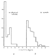
Figure 1: The radial distribution of elliptical and spiral “nebulae” in the Virgo cluster. The enhanced clustering of elliptical galaxies is apparent, and is used to construct many modern cluster catalogs.

However, the true pioneering work in this field did not come until 1957, upon the publication of a catalog of galaxy clusters produced by George Abell as his Caltech Ph.D. thesis, which appeared in the literature the following year (Abell 1958). Zwicky followed suit a decade later, with his voluminous Catalogue of Galaxies and of Clusters of Galaxies (Zwicky, Herzog & Wild 1968). However, Abell’s catalog remained the most cited and utilized resource for both galaxy population and cosmological studies with clusters for over forty years. Abell used the red plates of the first National Geographic-Palomar Observatory Sky Survey. These plates, each spanning $\sim 6^{\circ}$ on a side, covered the entire Northern sky, to a magnitude limit of $m_{r}\sim 20$. His extraordinary work required the visual measurement and cataloging of hundreds of thousands of galaxies To select clusters, Abell applied a number of criteria in an attempt to produce a fairly homogeneous catalog. He required a minimum number of galaxies within two magnitudes of the third brightest galaxy in a cluster ($m_{3}+2$), a fixed physical size within which galaxies were to be counted, a maximum and minimum distance to the clusters, and a minimum galactic latitude to avoid obscuration by interstellar dust. The resulting catalog, consisting of 1,682 clusters in the statistical sample, remained the only such resource until 1989. In that year, Abell, Corwin & Olowin (hereafter ACO) published an improved and expanded catalog, now including the Southern sky. These catalogs have been the foundation for many cosmological studies over the last four decades, even with serious questions about their reliability. Despite the numerical criteria laid out to define clusters in the Abell and ACO catalogs, their reliance on the human eye and use of older technology and a single filter led to various biases. These include a bias towards centrally-concentrated clusters (especially those with cD galaxies), a relatively low redshift cutoff ($z\sim 0.15$; Bahcall & Soneira 1983), and strong plate-to-plate sensitivity variations. Photometric errors and other inhomogeneities in the Abell catalog (Sutherland 1988, Efstathiou et al.1992), as well as projection effects (Lucey 1983, Katgert et al.1996) are a serious and difficult-to-quantify issue. These resulted in early findings of excess large-scale power in the angular correlation function (Bahcall & Soneira 1983), and later attempts to disentangle these issues relied on models to decontaminate the catalog (Sutherland 1988, Olivier et al.1990). The extent of these effects is also surprisingly unknown; measures of completeness and contamination in the Abell catalog disagree by factors of a few. For instance, Miller, Batuski & Slinglend (1999) claim that under- or over-estimation of richness is not a significant problem, whereas van Haarlem, Frenk & White (1997) suggest that one-third of Abell clusters have incorrect richnesses, and that one-third of rich ($R\geq 1$) clusters are missed. Unfortunately, some of these problems will plague any optically selected cluster sample, but objective selection criteria and a strong statistical understanding of the catalog can mitigate their effects.

In addition to the Zwicky and Abell catalogs, a few others based on plate material have also been produced, such as Shectman (1985), from the galaxy counts of Shane & Wirtanen (1954), and a search for more distant clusters carried out on plates from the Palomar $200^{\prime\prime}$ by Gunn, Hoessel & Oke (1986; hereafter GHO). None of these achieved the level of popularity of the Abell catalog, although the GHO survey was one of the first to detect a significant number of clusters at moderate to high redshifts ($0.15<z<0.9$), and remains in use to this day.

3 Hybrid Photo-Digital Surveys

Only in the past ten years has it become possible to utilize the objectivity of computational algorithms in the search for galaxy clusters. These more modern studies required that plates be digitized, so that the data are in machine readable form. Alternatively, the data had to be digital in origin, coming from CCD cameras. Unfortunately, this latter option provided only small area coverage, so the hybrid technology of digitized plate surveys blossomed into a cottage industry, with numerous catalogs being produced in the past decade. All such catalogs relied on two fundamental data sets: the Southern Sky Survey plates, scanned with the Automatic Plate Measuring (APM) machine (Maddox et al.1990) or COSMOS scanner (to produce the Edinburgh/Durham Southern Galaxy Catalog / EDSGC, Heydon-Dumbleton, Collins & MacGillivray 1989), and the POSS-I, scanned by the APS group (Pennington et al.1993). The first objective catalog produced was the Edinburgh/Durham Cluster Catalog (EDCC, Lumsden et al.1992), which covered 0.5 sr ($\sim 1,600$ square degrees) around the South Galactic Pole (SGP). Later, the APM cluster catalog was created by applying Abell-like criteria to select overdensities from the galaxy catalogs, and is discussed in detail in Dalton et al.(1997). More recent surveys, such as the EDCCII (Bramel, Nichol & Pope 2000) did not achieve the large area coverage of DPOSS (see below), and perhaps more importantly, are not nearly as deep. For instance, the EDCCII’s limiting magnitude is $b_{J}=20.5$. For an $L_{*}$ elliptical this corresponds to a limiting redshift of $z\sim 0.23$. The work by Odewahn & Aldering (1995), based on the POSS-I, provided a Northern sky example of such a catalog, while utilizing additional information (namely galaxy morphology). Some initial work on this problem, using higher quality POSS-II data, was performed by Picard (1991) in his thesis.

The largest, most recent, and likely the last photo-digital cluster survey is the Northern Sky Optical Survey (NoSOCS; Gal et al.2000, 2003, 2006; Lopes et al.2004). This survey relies on galaxy catalogs created from scans of the second generation Palomar Sky Survey plates. The POSS-II (Reid et al.1991) covers the entire northern sky ($\delta>-3^{\circ}$) with 897 overlapping fields (each $6.5^{\circ}$ square, with $5^{\circ}$ spacings), and, unlike the old POSS-I, has no gaps in the coverage. Approximately half of the survey area is covered at least twice in each band, due to plate overlaps. Plates are taken in three bands: blue-green, IIIa-$J$ + GG395, $\lambda_{\rm eff}\sim 480nm$; red, IIIa-$F$ + RG610, $\lambda_{\rm eff}\sim 650nm$; and very near-IR, IV-$N$ + RG9, $\lambda_{\rm eff}\sim 850nm$. Typical limiting magnitudes reached are $B_{J}\sim 22.5$, $R_{F}\sim 20.8$, and $I_{N}\sim 19.5$, i.e. , $\sim 1^{m}-1.5^{m}$ deeper than POSS-I. The image quality is improved relative to POSS-I, and is comparable to the southern photographic sky surveys. The original survey plates are digitized at STScI, using modified PDS scanners (Lasker 1996). The plates are scanned with $15\mu$ ($1.0^{\prime\prime}$) pixels, in rasters of 23,040 square, giving $\sim 1$ GB/plate, or $\sim 3$ TB of pixel data total for the entire digital survey. The digital scans are processed, calibrated, and cataloged, with detection of all objects down to the survey limit, and star/galaxy classifications accurate to 90% or better down to $\sim 1^{m}$ above the detection limit (Odewahn et al.2004). They are photometrically calibrated using extensive CCD observations of Abell clusters (Gal et al.2004a).

The resulting galaxy catalogs are used as an input to an adaptive kernel galaxy density mapping routine (discussed in §5), and photometric redshifts based on galaxy colors are calculated, along with cluster richnesses in a fixed absolute luminosity interval. The NoSOCS survey utilizes $F$ (red) plates, with a limiting magnitude of $m_{r}=20$. This corresponds to a limiting redshift of 0.33 for an $L_{*}$ elliptical galaxy. Because of the increase in $g-r$ color with redshift, the APM would have to go as deep as $b_{J}=22.0$ to reach the same redshift from their data for early type galaxies. Similarly, even at lower redshift, this implies that DPOSS can see $\sim 0.5^{m}-1^{m}$ deeper in the cluster luminosity functions. Additionally, NoSOCS uses at least one color (two filters), and a significantly increased amount of CCD photometric calibration data. The final catalog covers 11,733 square degrees, with nearly 16,000 candidate clusters (Figure 2), extending to $z\sim 0.3$, making it the largest such resource in existence. However, new CCD surveys, discussed in the next section, are about to surpass even this benchmark.

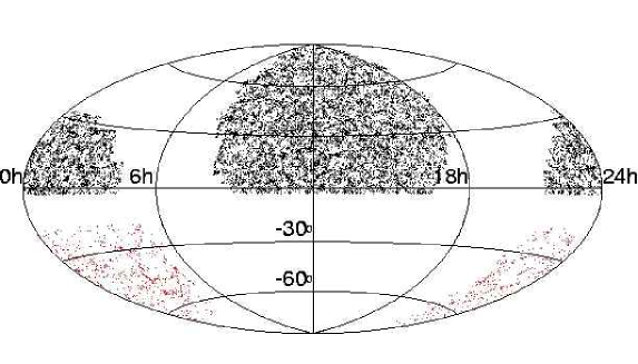
Figure 2: The sky distribution of NoSOCS (northern sky) and APM (southern sky) candidate clusters in equatorial coordinates. The much higher density of NoSOCS is due to its deeper photometry and lower richness limit.

4 Digital CCD Surveys

With the advent of charge-coupled devices (CCDs), fully digital imaging in astronomy became a reality. These detectors provided an order-of-magnitude increase in sensitivity, linear response to light, small pixel size, stability, and much easier calibration. The main drawback relative to photographic plates was (and remains) their small physical size, which permits only a small area (of order $10^{\prime}$) to be imaged by a typical $2048^{2}$ pixel detector. As detector sizes grew, and it became possible to build multi-detector arrays covering large areas, it became apparent that new sky surveys with this modern technology could be created, far surpassing their photographic precursors. Unfortunately, in the 1990s most modern telescopes did not provide large enough fields-of-view, and building a sufficiently large detector array to efficiently map thousands of square degrees was still challenging.

Nevertheless, realizing the vast scientific potential of such a survey, an international collaboration embarked on the Sloan Digital Sky Survey (SDSS, York et al.2000), which included construction of a specialized 2.5 meter telescope, a camera with a mosaic of 30 CCDs, a 640-fiber multi-object spectrograph, a novel observing strategy, and automated pipelines for survey operations and data processing. Main survey operations were completed in the fall of 2005, with over 8,000 square degrees of the northern sky image in five filters to a depth of $r^{\prime}\sim 22.2$ with calibration accurate to $\sim 2-3\%$, as well as spectroscopy of nearly one million objects.

With such a rich dataset, many groups both internal and external to the SDSS collaboration have generated a variety of cluster catalogs, from both the photometric and the spectroscopic catalogs, using techniques including:

1. Voronoi Tessellation (Kim et al.2002)

2. Overdensities in both spatial and color space (maxBCG, Annis et al.1999)

3. Subdividing by color and making density maps (Cut-and-Enhance, Goto et al.2002)

4. The Matched Filter and its variants (Kim et al.2002)

5. Surface brightness enhancements (Bartelmann et al.2002, Zaritsky et al.1997, 2002)

6. Overdensities in position and color spaces, including redshifts (C4; Miller et al.2005)

These techniques are described in more detail in §5. Each method generates a different catalog, and early attempts to compare them have shown not only that the catalogs are quite distinct, but also that comparison of two photometrically-derived catalogs, even from the same galaxy catalogs, is not straightforward (Bahcall et al.2003).

In addition to the SDSS, smaller areas, to much higher redshift, have been covered by numerous deep CCD imaging surveys. Notable examples include the Palomar Distant Cluster Survey (PDCS, Postman et al.1996), the ESO Imaging Survey (EIS, Lobo et al.2000), Zaritsky et al.(1997), and many others. None of these surveys provide the angular coverage necessary for large-scale structure and cosmology studies, and are specifically designed to find rich clusters at high redshift. The largest such survey to date is the Red Sequence Cluster Survey (RCS, Gladders et al.2005), based on moderately deep two-band imaging using the CFH12K mosaic camera on the CFHT 3.6m telescope, covers $\sim 100$ square degrees. This area coverage makes it comparable to or larger than X-ray surveys designed to detect clusters at $z\sim 1$. The use of the red sequence of early-type galaxies makes this a very efficient survey, and the methodology is described is §5.

5 Algorithms

From our earlier discussion, it is obvious that many different mathematical and methodological choices must be made when embarking on an optical cluster survey. Regardless of the dataset and algorithms used, a few simple rules should be followed to produce a catalog that is useful for statistical studies of galaxy populations and for cosmological tests:

1. Cluster detection should be performed by an objective, automated algorithm to minimize human biases and fatigue.

2. The algorithm utilized should impose minimal constraints on the physical properties of the clusters, to avoid selection biases. If not, these biases must be properly characterized.

3. The sample selection function must be well-understood, in terms of both completeness and contamination, as a function of both redshift and richness. The effects of varying the cluster model on the determination of these functions must also be known.

4. The catalog should provide basic physical properties for all the detected clusters, including estimates of their distances and some mass-related quantity (richness, luminosity, overdensity) such that specific subsamples can be selected for future study.

This section describes many of the algorithms used to detect clusters in modern cluster surveys. No single one of these generates an ’optimal’ cluster catalog, if such a thing can even be said to exist. Therefore, I provide some of the strengths and weaknesses of each technique. In addition to the methods discussed here, many other variants are possible, and in the future, joint detection at multiple wavelengths (i.e. optical and X-ray, Schuecker et al.2004) may yield more complete samples to higher redshifts and lower mass limits, with less contamination.

5.1 Counts in Cells

The earliest cluster catalogs, like those of Abell, utilized a simple technique of counting galaxies in a fixed magnitude interval, in cells of a fixed physical or angular size. Indeed, Abell simply used visual recognition of galaxy overdensities, whose properties were then measured ex post facto in fixed physical cells. This technique was used by Couch et al.(1991) and Lidman & Peterson (1996) to detect clusters at moderate redshifts ($z\sim 0.5$), by requiring a specified enhancement, above the mean background, of the galaxy surface density in a given area. This enhancement, called the contrast, is defined as

$${\sigma_{cl}={N_{cluster}-N_{field}\over\sigma_{field}}}$$ (1)

where $N_{cluster}$ is the number of galaxies in the cell corresponding to the cluster, $N_{field}$ is the mean background counts and $\sigma_{field}$ is the variance of the field counts for the same area. The magnitude range and cell size used are parameters that must be set based on the photometric survey material and the type or distance of clusters to be found. For instance, Lidman & Peterson (1996) chose these parameters to maximize the contrast above background for a cluster at $z=0.5$. Using the distribution of cell counts, one can analytically determine the detection likelihood of a cluster with a given redshift and richness (assuming a fixed luminosity function), given a detection threshold. The false detection rate is harder, if not impossible, to quantify, without running the algorithm on a catalog with extensive spectroscopy. This is true for most of the techniques that rely on photometry alone. It is also possible to increase the contrast of clusters with the background by weighting galaxies based on their luminosities and positions. Galaxies closer to the cluster center are upweighted, while the luminosity weighting depends on both the cluster and field luminosity functions, as well as the cluster redshift. This scheme is similar to that used by the matched filter algorithm, detailed later.

This technique, although straightforward, has numerous drawbacks. First, it relies on initial visual detection of overdensities, which are then quantified objectively. Since simple counts-in-cells methods use the galaxy distribution projected along the entire line of sight, chance alignments of poorer systems become more common, increasing the contamination. Optimizing the magnitude range and cell size for a given redshift reduces the efficiency of detecting clusters at other redshifts, especially closer ones since their core radii are much larger. Setting the magnitude range typically assumes that the cluster galaxy luminosity function at the redshift of interest is the same as it is today, which is not true. Furthermore, single band surveys observe different portions of the rest frame spectrum of galaxies at different redshifts, altering the relative sensitivity to clusters over the range probed. Finally, the selection function can only be determined analytically for circular clusters with fixed luminosity functions. Given these issues, this technique is inappropriate for modern, deep surveys.

5.2 Percolation Algorithms

A majority of current cluster surveys rely on a smoothed map of projected galaxy density from which peaks are selected (see below). However, smoothing invariable reduces the amount of information being used, leading some authors to employ percolation (or friends-of-friends, FOF) algorithms. In their simplest form, these techniques link pairs of galaxies that are separated by a distance less than some threshold (typically related to the mean galaxy separations). Galaxies that have links in common are then assigned to the same group; once a group contains more than a specified number of members, it becomes a candidate cluster. This technique was used by Dalton et al.(1997) to construct a cluster catalog from APM data. However, it is not typically used on two dimensional data, because the results of this method are very sensitive to the linking length, and can easily combine multiple clusters into long, filamentary structures. On the other hand, FOF algorithms are very commonly used for structure finding in three-dimensional data, especially N-body simulations (Davis et al.1985, Efstathiou et al.1988) and redshift surveys (Huchra & Geller 1982, Ramella et al.2002). A variant of this technique utilizing photometric redshifts has been recently proposed by Botzler et al.(2004).

5.3 Simple Smoothing Kernels

Another objective and automated approach to cluster detection is the use of a smoothing kernel to generate a continuous density field from the discrete positions of galaxies in a catalog. For instance, Shectman (1985) used the galaxy counts of Shane & Wirtanen in $10^{\prime}$ bins, smoothed with a very simple weighting kernel. A minimum number of galaxies within this smoothed region (in this case, 20) were then required to detect a cluster. This type of kernel is fixed in angular size and thus does not smooth clusters at different redshifts with consistent physical radii, making its sensitivity highly redshift dependent. Similarly, it uses the full projected galaxy distribution (much as Abell did), and is thus insensitive to the different parts of the LF sampled at different redshifts.

5.4 The Adaptive Kernel

A slightly more sophisticated technique is to use an adaptive smoothing kernel (Silverman 1986). This technique uses a two–stage process to produce a density map. First, at each point $t$, it produces a pilot estimate $f(t)$ of the galaxy density at each point in the map. Based on this pilot estimate, it then applies a smoothing kernel whose size changes as a function of the local density, with a smaller kernel at higher density. This is achieved by defining a local bandwidth factor:

$${\lambda_{i}=[f(t)/g]^{-\alpha},}$$ (2)

where $g$ is the geometric mean of $f(t)$ and $\alpha$ is a sensitivity parameter that sets the variation of kernel size with density. NoSOCS uses a sensitivity parameter $\alpha=0.5$, which results in a minimally biased final density estimate, and is simultaneously more sensitive to local density variations than a fixed–width kernel (Silverman 1986). This is then used to construct the adaptive kernel estimate:

$${\hat{f}(t)=n^{-1}\sum_{i=1}^{n}h^{-2}\lambda_{i}^{-2}K\{h^{-2}\lambda_{i}^{-2}(t-X_{i})\}}$$ (3)

where $h$ is the bandwidth, which is a parameter that must be set based on the survey properties.

The adaptive kernel was used to generate the Northern Sky Optical Cluster Survey (Gal et al.2000, 2003, 2006). The smoothing size (in their case, $500^{\prime\prime}$ radius) is set to prevent over–smoothing the cores of higher redshift ($z\sim 0.3$) clusters, while avoiding fragmentation of most low redshift ($z\sim 0.08$) clusters. Because the input galaxy catalog is relatively shallow, and the redshift range probed is not very large, it is possible to do this. For deeper surveys, this is not practical, and therefore this technique cannot be used in its simplest form. Figure 3 demonstrates example density maps, showing the effect of varying the initial smoothing window. In this figure, four simulated clusters are placed into a simulated background, representing the expected range of detectability in the NoSOCS survey. There are two clusters at low $z$ (0.08), and two at high $z$ (0.24), with one poor and one rich cluster at each redshift (100 and 333 total members, $N_{gals}=25$ and 80 respectively).

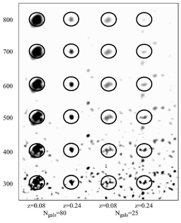
Figure 3: The effect of varying the initial smoothing window for the adaptive kernel on cluster appearance. Each panel contains a simulated background with four simulated clusters, as described in the text. The smoothing kernel ranges in size from $300^{\prime\prime}$ to $800^{\prime\prime}$ in $100^{\prime\prime}$ increments. Taken from Gal et al.(2003).

After a smooth density map is generated, cluster detection can be performed analogously to object detection in standard astronomical images. In NoSOCS, Gal et al.used SExtractor (Bertin & Arnouts 1996) to detect density peaks. The tuning of parameters in the detection step is fundamentally important in such surveys, and can be accomplished using simulated clusters placed in the observed density field, from which the completeness and false detection rates can be determined. Even so, this method involves many adjustable parameters (the smoothing kernel size, sensitivity parameter, and all the source detection parameters) such that it must be optimized with care for the data being used. Given an end-to-end cluster detection methodology, one can use simulations to determine the selection function’s dependence on redshift, richness, and other cluster properties (see Gal et al.2003 for details). However, the measurement of cluster richness and redshift are done in a step separate from detection, using the input galaxy catalogs, further complicating this technique. The adaptive kernel is very fast and simple to implement, making it suitable for all–sky surveys, but is only truly useful in situations where the photometry is poor, and the survey is not very deep, as is the case for NoSOCS.

5.5 Surface Brightness Enhancements

It is not necessary to have photometry for individual galaxies to detect clusters. A novel but difficult approach is to detect the localized cumulative surface brightness enhancement due to unresolved light from galaxies in distant clusters. This method was pioneered by Zaritsky et al.(1997, 2001), who showed that distant clusters could be detected using short integration times on small 1-m class telescopes. However, this method requires extremely accurate flat-fielding, object subtraction, masking of bright stars. and excellent data homogeneiety. Once all detected obejcts are removed from a frame, and nuisance sources such as bright stars masked, the remaining data is smoothed with a kernel comparable to the size of clusters at the desired redshift. The completeness and contamination rates of such a catalog are extremely difficult to model. Thus, this technique is not necessarily appropriate for generating statistical catalogs for cosmological tests, but is an excellent, cost-effective means to find interesting objects for other studies.

5.6 The Matched Filter

With accurate photometry, and deeper surveys, one can use more sophisticated tools for cluster detection. As we will discuss later, color information is very powerful, but is not always available. However, even with single–band data, it is possible to simultaneously use the locations and magnitudes of galaxies. One such method is the matched filter (Postman et al.1996), which models the spatial and luminosity distribution of galaxies in a cluster, and tests how well galaxies in a given sky region match this model for various redshifts. As a result, it outputs an estimate of the redshift and total luminosity of each detected cluster as an integral part of the detection scheme. Following Postman et al.we can describe, at any location, the distribution of galaxies per unit area and magnitude $D(r,m)$ as a sum of the background and possible cluster contributions:

$${D(r,m)=b(m)+\Lambda_{cl}P(r/r_{c})\phi(m-m^{*})}$$ (4)

Here, D is the number of galaxies per magnitude per arcsec² at magnitude $m$ and distance $r$ from a putative cluster center. The background density is $b(m)$, and the cluster contribution is defined by a parameter $\Lambda_{cl}$ proportional to its total richness, its differential luminosity function $\phi(m-m^{*})$, and its projected radial profile $P(r/r_{c})$. The parameter $r_{c}$ is the characteristic cluster radius, and $m^{*}$ is the characteristic galaxy luminosity. One can then construct a likelihood for the data given this model, which is a function of the parameters $r_{c}$,$m^{*}$, and $\Lambda_{cl}$. Because two of these parameters, especially $m^{*}$, are sensitive to the redshift, one obtains an estimated redshift when maximizing the likelihood relative to this parameter. The algorithm outputs the richness $\Lambda_{cl}$ at each redshift tested, and thus provides an integrated estimator of the total cluster richness. The luminosity function used by Postman et al.is a Schechter (1976) function with a power law cutoff applied to the faint end, while they use a circularly symmetric radial profile with core and cutoff radii (see their eqn. 19).

Like the adaptive kernel, this method produces density maps on which source detection must still be run. These maps have a grid size set by the user, typically of order half the core radius at each redshift used, with numerous maps for each field, one for each redshift tested. The goal of the matched filter is to improve the contrast of clusters above the background, by convolving with an ’optimal’ filter, and also to output redshift and richness estimates. Given a set of density maps, one can use a variety of detection algorithms to select peaks. A given cluster is likely to be detected in multiple maps (at different redshifts) of the same region; its redshift is estimated by finding the filter redshift at which the peak signal is maximized. By using multiple photometric bands, one can run this algorithm separately on each band and improve the reliability of the catalogs. The richness of a cluster is measured from the density map corresponding to the cluster redshift, and represents approximately the equivalent number of $L_{*}$ galaxies in the cluster.

The matched filter is a very powerful cluster detection technique. It can handle deep surveys spanning a large redshift range, and provides redshift and richness measures as an innate part of the procedure. The selection function can be estimated using simulated clusters, as was done in significant detail by Postman et al.However, the technique relies on fixed analytic luminosity functions and radial profiles for the likelihood estimates. Thus, clusters which have properties inconsistent with these input functions will be detected at lower likelihood, if at all. While this is not likely to be an issue at low to moderate redshifts, as the population of clusters becomes increasingly merger dominated at $z\sim 0.8$ (Cohn et al.2005), these simple representations will fail. Similarly, the cluster and field LF both evolve with redshift, which can effect the estimated redshift. Also, as the redshifts and $k$-corrections become large, one samples a very different region of the LF than at low redshift. Nevertheless, this remains one of the best cluster detection techniques for cluster detection in moderately deep surveys.

5.7 Hybrid and Adaptive Matched Filter

The matched filter can be extended to include estimated (photometric) or measured (spectroscopic) redshifts. This extension has been called the adaptive matched filter (AMF, Kepner et al.1999). The adaptive here refers to this method’s ability to accept 2-dimensional (positions and magnitudes), 2.5-dimensional (positions, magnitudes, and estimated redshifts), and 3-dimensional (positions, magnitudes, and redshifts) data, adapting to the redshift errors. In implementation, this technique uses a two–stage method, first maximizing the cluster likelihood on a coarse grid of locations and redshifts, and then refining the redshift and richness on a finer grid. Unlike the standard matched filter, the AMF evaluates the likelihood function at each galaxy position, and not on a fixed grid for each redshift interval. Thus, for each galaxy, the output includes a likelihood that there is a cluster centered on this galaxy, and the estimated redshift.

The inclusion of photometric redshifts should substantially improve detection of poor clusters, which is very important since most galaxies live in poor systems, and these are suspected to be sites for significant galaxy evolution. However, Kim et al.(2002), using SDSS data, found that the simple matched filter is more efficient at detecting faint clusters, while the AMF estimated cluster properties more accurately. The matched filter performs better for detection because the significance threshold for finding candidates is redshift dependent, determined separately for each map produced in different redshift intervals. The AMF, on the other hand, finds peaks first in redshift space, and then selects candidates using a universal threshold. Thus, they propose a hybrid system, using the matched filter to detect candidate clusters, and the AMF to obtain its properties.

5.8 Cut-and-Enhance

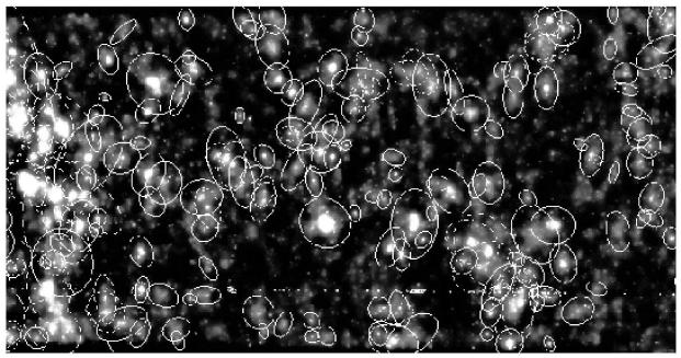
Figure 4: An enhanced map of the galaxy distribution in the SDSS Early Data Release, after applying the $g*-r*-i*$ color-color cut. Detected clusters are circled. Taken from Goto et al.(2002).

Despite the popularity of matched filter algorithms for cluster detection, their assumption of a radial profile and luminosity function are cause for concern. Thus, development of semi-parametric detection methods remains a vibrant area of research. While the adaptive kernel described earlier is such a technique, more sophisticated algorithms are possible, especially with the inclusion of color information. One such technique is the Cut-and-Enhance method (Goto et al.2002), which has been applied to SDSS data. This method relies on the presence of the red sequence in clusters, applying a variety of color and color-color cuts to generate galaxy subsamples which should span different redshift ranges. Within each cut, pairs of galaxies with separations less than $5^{\prime}$ are replaced by Gaussian clouds, which are then summed to generate density maps. In this technique, the presence of many close pairs (as in a high redshift cluster) yields a more compact cloud, making it easier to detect, and thus possibly biasing the catalog against low-$z$ clusters. As with the AK technique, this method yields a density map on which object detection must be performed; Goto et al.(2002) utilize SExtractor. Once potential clusters are detected in the maps made using the various color cuts, these catalogs must be merged to produce a single list of candidates. Redshift and richness estimates are performed a posteriori, as they are with the AK. Similar to the AK, there are many tunable parameters which make this method difficult to optimize.

5.9 Voronoi Tessellation

Figure 5: Voronoi Tessellation of galaxies with $17.0\leq m_{r}\leq 18.5$ in a DPOSS field. Each triangle represents a galaxy surrounded by its associated Voronoi cell (indicated by the polyhedrals). Excised areas (due to bright objects) are shown as rectangles. Taken from Lopes et al.(2004)

Considering a distribution of particles it is possible to define a characteristic volume associated with each particle. This is known as the Voronoi volume, whose radius is of the order of the mean particle separation. The complete division of a region into these volumes is known as Voronoi Tessellation (VT), and it has been applied to a variety of astronomical problems, and in particular to cluster detection by Kim et al.(2002) and Ramella et al.(2001). As pointed out by the latter, one of the main advantages of employing VT to look for galaxy clusters is that this technique does not distribute the data in bins, nor does it assume a particular source geometry intrinsic to the detection process. The algorithm is thus sensitive to irregular and elongated structures.

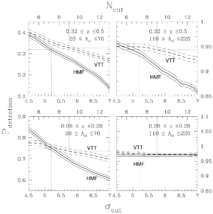
Figure 6: The absolute recovery rates of clusters from the SDSS in four different ranges of cluster parameters for the HMF (solid line) and the VTT (dashed line). Taken from Kim et al.(2002).

The parameter of interest in this case is the galaxy density. When applying VT to a galaxy catalog, each galaxy is considered as a seed and has a Voronoi cell associated to it. The area of this cell is interpreted as the effective area a galaxy occupies in the plane. The inverse of this area gives the local density at that point. Galaxy clusters are identified by high density regions, composed of small adjacent cells, i.e. , cells small enough to give a density value higher than the chosen density threshold. An example of Voronoi Tessellation applied to a galaxy catalog for one DPOSS field is presented in Figure 5. For clarity, we show only galaxies with $17.0\leq m_{r}\leq 18.5$.

Figure 7: Richness (top) and estimated redshift (bottom) distributions for clusters detected in DPOSS by only the VT code (dash-dotted line), only the AK code (dotted line), and by both methods (heavy solid line). Taken from Lopes et al.(2004).

Once such a tessellation is created, candidate clusters are identified based on two criteria. The first is the density threshold, which is used to identify fluctuations as significant overdensities over the background distribution, and is termed the search confidence level (scl). The second criterion rejects candidates from the preliminary list using statistics of Voronoi Tessellation for a poissonian distribution of particles, by computing the probability that an overdensity is a random fluctuation. This is called the rejection confidence level (rcl). Kim et al.(2002) used the color–magnitude relation for cluster ellipticals to divide the galaxy catalog into separate redshift bins, and ran the VT code on each bin. Candidates in each slice are identified by requiring a minimum number $N_{hdg}$ of galaxies having overdensities $\delta$ greater than some threshold $\delta_{c}$, within a radius of 0.7$h^{-1}$ Mpc. The candidates originating in different bins are then cross-correlated to filter out significant overlaps and produce the final catalog. Ramella et al.(2001) and Lopes et al.(2004) follow a different approach, as they do not have color information. Instead, they use the object magnitudes to minimize background/foreground contamination and enhance the cluster contrast, as follows:

1. The galaxy catalog is divided into different magnitude bins, starting at the bright limit of the sample and shifting to progressively fainter bins. The step size adopted is derived from the photometric errors of the catalog.

2. The VT code is run using the galaxy catalog for each bin, resulting in a catalog of cluster candidates associated with each magnitude slice.

3. The centroid of a cluster candidate detected in different bins will change due to the statistical noise of the foreground/background galaxy distribution. Thus, the cluster catalogs from all bins are cross-matched, and overdensities are merged according to a set criterion, producing a combined catalog.

4. A minimum number (N_min) of detections in different bins is required in order to consider a given fluctuation as a cluster candidate. N_min acts as a final threshold for the whole procedure. After this step, the final cluster catalog is complete.

Kim et al.(2002) and Lopes et al.(2004) compare the performance of their VT algorithms with the HMF and adaptive kernel, respectively. Figure 6 (taken from Kim et al.2002) shows the absolute recovery rates of clusters in four different ranges of cluster parameters for the HMF (solid line) and the VT (dashed line). Both algorithms agree very well for clusters with the highest signals (rich, low redshift), but the VT does slightly better for the thresholds determined from the uniform background case. Similarly, Lopes et al.(2004) find that the VT algorithm performs better for poor, nearby clusters, while the adaptive kernel goes deeper when detecting rich systems, as seen in Figure 7, where the VT-only detections are preferentially poor and low redshift, and the AK-only detections are richer and at high redshift.

5.10 maxBCG

The maxBCG algorithm, developed for use on SDSS data (Annis et al. 2002, Hansen et al.2005), is another technique that relies on the small color dispersion of early–type cluster galaxies. The brightest of the cluster galaxies (BCGs) have predictable colors and magnitudes out to redshifts of order unity. Unlike many of the other techniques discussed above, maxBCG does not generate density maps. Instead, it calculates a likelihood as a function of redshift for each galaxy that it is a BCG, based on its colors and the presence of a red sequence from the surrounding objects. This is calculated as

$${{\mathcal{L}}_{max}=max{\mathcal{L}}(z);{\mathcal{L}}(z)={\mathcal{L}}_{BCG}+\log N_{gal}}$$ (5)

where ${\mathcal{L}}_{BCG}$ is the likelihood, at redshift $z$, that a galaxy is a BCG, based on its colors and luminosity, and $N_{gal}$ is the number of galaxies within 1 $h^{-1}$ Mpc with colors and magnitudes consistent with the red sequence (i.e. within 0.1 mag of the mean BCG color at the redshift being tested). This procedure results in a maximum likelihood and redshift for each galaxy in the catalog. The peaks in the ${\mathcal{L}}_{max}$ distribution are then selected as the candidate clusters.

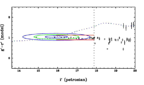
Figure 8: SDSS color–magnitude diagram of observed $g-r$ vs. apparent $i$ band for galaxies near a rich cluster at $z$ = 0.15. Ellipses represent 1, 2, and 3 $\sigma$ contours around the mean BCG color and magnitude at that redshift. The dotted line indicates the track of BCG color and magnitude as a function of redshift. The horizontal lines and vertical dashed line show the region of inclusion for $N_{gal}$ determination. Taken from Hansen et al.(2005).

This algorithm appears to be extremely powerful for selecting clusters in the SDSS. Simulations suggest that maxBCG recovers and correctly estimates the richness for greater than 90% of clusters and groups present with $N_{gal}\geq 15$ out to $z=0.3$, with an estimated redshift dispersion of $\delta z=0.02$. As long as one can obtain a sufficiently deep photometric catalog, with the appropriate colors to map the red sequence, this technique can be used to very efficiently detect clusters. Like all methods that rely on the presence of a red sequence, it will eventually fail at sufficiently high redshifts, where the cluster galaxy population becomes more heterogeneous. However, clusters detected out to $z\sim 1-1.5$, even using non-optical techniques, still show a red sequence, albeit with larger scatter, which will reduce the efficiency of this method. Additionally, the definition of $N_{gals}$ as the number of red sequence galaxies may introduce a bias, as poorer, less concentrated, or more distant clusters have less well defined color–magnitude relations, and the luminosity functions for clusters vary with richness as well (Figure 10 of Hansen et al.2005).

5.11 The Cluster Red Sequence Method

As we have discussed already, the existence of a tight color–magnitude relation for cluster galaxies provides a mechanism for reducing fore- and background contamination, enhancing cluster contrast, and estimating redshifts in cluster surveys. Because the red sequence is such a strong indicator of a cluster’s presence, and is especially tight for the brighter cluster members, it can be used to detect clusters to high redshifts ($z\sim 1$) with comparatively shallow imaging, if an optimal set of photometric bands is chosen. This is the idea behind the Cluster Red Sequence (CRS; Gladders & Yee 2000) method, utilized by the Red Sequence Cluster Survey (RCS; Gladders et al.2005). Figure 9a shows model color–magnitude tracks for different galaxy types for $0.1\leq z\leq 1.0$. The cluster ellipticals are the reddest objects at all redshifts. Even more importantly, if the filters used straddle the 4000Å break at a given redshift, the cluster ellipticals at that redshift are redder than all galaxies at all lower redshifts. The only contaminants are more distant, bluer galaxies, eliminating most of the foreground contamination found in imaging surveys. The change of the red sequence color with redshift at a fixed apparent magnitude also makes it a very useful redshift estimator (López-Cruz 2004).

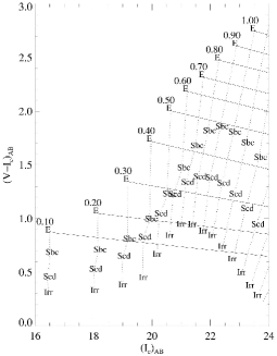
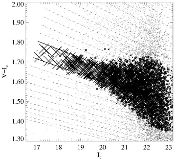
Figure 9: Left: Simulated $(V-I_{c})_{AB}$ vs. $(I_{c})_{AB}$ color–magnitude diagram. Model apparent magnitudes and colors at various redshifts for several types of galaxies at a fixed $M_{I}$ of -22 are shown. The dotted lines connect galaxies at the same redshift. Solid near-horizontal lines show the expected slope of the red sequence at each redshift. Right: CMD of a CNOC2 Redshift Survey Patch, with dashed lines showing various color CRS slices. The galaxy symbols are sized by the probability that they belong to the color slice defined by the solid lines. Taken from Gladders & Yee (2000).

Gladders & Yee generate a set of overlapping color slices based on models of the red sequence. A subset of galaxies is selected that belong to each slice, based on their magnitudes, colors, color errors, and the models. A weight for each chosen galaxy is computed, based on the galaxy magnitude and the likelihood that the galaxy belongs to the color slice in question (Figure 9b). A surface density map is then constructed for each slice using a fixed smoothing kernel, with a scale radius of 0.33 $h^{-1}$ Mpc. All the slices taken together form a volume density in position and redshift. Peaks are then selected from this volume. Gladders et al.2005 present the results of this technique applied to the first two RCS patches.

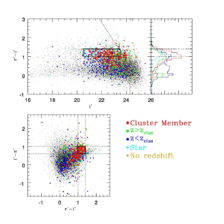
Figure 10: $r-i$ vs. $i$ color–magnitude and $r-i$ vs. $i-z$ color–color diagrams for objects in the Cl1604 field.

In a similar vein, the High Redshift Large Scale Structure Survey (Lubin et al.2006, Gal et al.2004b, 2005) uses deep multicolor photometry around known clusters at $z>0.7$ to search for additional large scale structure. They apply color and color–color cuts to select galaxies with the colors of spectroscopically confirmed members in the original clusters. The selected galaxies are used to make adaptive kernel density maps from which peaks are selected. This technique was applied to the Cl1604 supercluster at $z\sim 0.9$. Starting with two known clusters with approximately 20 spectroscopic members, there are now a dozen structures with 360 confirmed members known in this supercluster. These galaxies typically follow the red sequence, but as can be seen in Figure 10, the scatter is very large, and many cluster or supercluster members are actually bluer than the red sequence at this redshift. Figure 10 shows the $r-i$ vs. $i$ color–magnitude and $r-i$ vs. $i-z$ color–color diagrams for objects in a $\sim 30^{\prime}$ square region around the Cl1604 supercluster, with all known cluster members shown in red. and the color selection boxes marked. Figure 11 shows the density map for this region, with two different significance thresholds, and the clusters comprising the supercluster marked. Clearly, in regions such as this, traditional cluster detection techniques will yield incorrect results, combining multiple clusters, and measuring incorrect redshifts and richnesses. Figure 12 shows a 3-d map of the spectroscopically confirmed supercluster members, revealing the complex nature of this structure. Dots are scaled with galaxy luminosity. While only $\sim 10$ Mpc across on the sky, the apparent depth of this structure is nearly 10 times greater, making it comparable to the largest local superclusters.

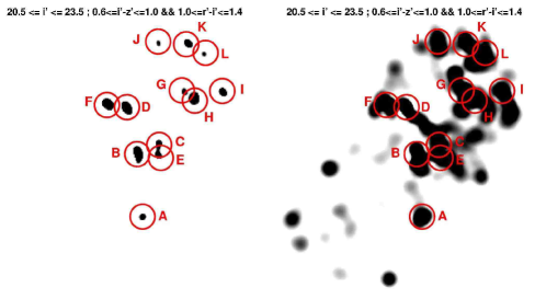
Figure 11: Density maps of galaxies meeting the $z\sim 0.9$ red galaxy criteria in the Cl1604 field .

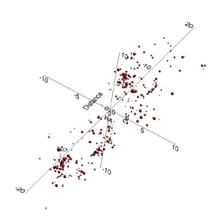
Figure 12: Three dimensional spatial distribution of the spectroscopically confirmed Cl1604 supercluster members. Dots are scaled by galaxy luminosity.

6 Conclusions

It is clear that there exist many methods for detecting clusters in optical imaging surveys. Some of these are designed to work on very simple, single–band data (AK, Matched Filter, VT), but will work on multicolor data as well. Others, such as maxBCG and the CRS method, rely on galaxy colors and the red sequence to potentially improve cluster detection and reduce contamination by projections and spurious objects. Very little work has been done to compare these techniques, with the exceptions of Kim et al.2001, Bahcall et al.(2003) and Lopes et al.(2004), each of whom compared the results of only two or three algorithms. Even from these tests it is clear that no single technique is perfect, although some (notably those that use colors) are clearly more robust. Certainly any program to find clusters in imaging data must consider the input photometry when deciding which, if any, of these methods to use.

One of the most vexing issues facing cluster surveys is our inability to compare directly to large scale cosmological simulations. Most such simulations are N-body only, but have perfect knowledge of object masses and positions. Thus, it is possible to construct algorithms to detect overdensities based purely on mass, but it is not possible to obtain the photometric properties of these objects! Recent work, such as the Millennium Simulation (Springel et al.2005), is approaching this goal. It is necessary to extract from these simulations the magnitudes of galaxies in filters used for actual surveys, and run the various cluster detection algorithms on these simulated galaxy catalogs. The results can then be compared to that of pure mass selection, and the redshift-, structure- and mass-dependent biases understood. Ideally, this should be done for many large simulations using different cosmologies, since the galaxy evolution and selection effects will vary. Such work is fundamental if we are to use the evolution of the mass function of galaxy clusters for cosmology. As deeper and larger optical surveys, such as LSST, and other techniques such as X-ray and Sunyaev–Z’eldovich effect observations become available, the need for these simulations becomes ever greater.

References

- (1) G. O. Abell: ApJS 3, 211 (1958)
- (2) G. O. Abell, H. G. Corwin, & R. P. Olowin: ApJS 70, 1 (1989)
- (3) J. Annis et al.: AAS 31, 1391 (1999)
- (4) N. A. Bahcall & R. M. Soneira: ApJ 270, 20 (1983)
- (5) N. A. Bahcall et al.: ApJS 148, 243 (2003)
- (6) E. Bertin & S. Arnouts: A&AS 117, 393 (1996)
- (7) C. S. Botzler et al.: MNRAS 349, 425 (2004)
- (8) D. A. Bramel, R. C. Nichol, & A. C. Pope: ApJ 533, 601 (2000)
- (9) J. D. Cohn & M. White: APh 24, 316 (2005)
- (10) W. J. Couch, et al.: MNRAS 249, 606 (1991)
- (11) G. B. Dalton et al.: MNRAS 289, 263 (1997)
- (12) M. Davis et al.: ApJ 292, 371 (1985)
- (13) G. Efstathiou et al.: MNRAS 235, 715 (1988)
- (14) G. Efstathiou et al.: MNRAS 257, 125 (1992)
- (15) R. R. Gal et al.: AJ 119, 12 (2000)
- (16) R. R. Gal et al.: AJ 125, 2064 (2003)
- (17) R. R. Gal et al.: AJ 128, 3082 (2004a)
- (18) R. R. Gal & L. M. Lubin: ApJ 607, L1 (2004b)
- (19) R. R. Gal, L. M. Lubin, & G. K. Squires: AJ 129, 1827 (2005)
- (20) R. R. Gal et al.: in prep. (2006)
- (21) M. D. Gladders & H. K. C. Yee: AJ 120, 2148 (2000)
- (22) M. D. Gladders & H. K. C. Yee: ApJS 157, 1 (2005)
- (23) T. Goto et al.: AJ 123, 1807 (2002)
- (24) J. E. Gunn, J. G. Hoessel, & J. B. Oke: ApJ 306, 30 (1986)
- (25) S. M. Hansen et al.: ApJ 633, 122 (2005)
- (26) N. H. Heydon-Dumbleton, C. A. Collins, & H. T. MacGillivray: MNRAS 238, 379 (1989)
- (27) J. P. Huchra & M. J. Geller: ApJ 257, 423 (1982)
- (28) P. Katgert et al.: A&A 310, 8 (1996)
- (29) L. Katz & G. F. W. Mulders: ApJ 95, 565 (1942)
- (30) J. Kepner et al.: ApJ 517, 78 (1999)
- (31) R. S. J Kim et al.: AJ 123, 20 (2002)
- (32) b. M. Lasker et al.: ASPC 101, 88 (1996)
- (33) C. E. Lidman & B. A. Peterson: AJ 112, 2454 (1996)
- (34) C. Lobo et al.: A&A 360, 896 (2000)
- (35) P. A. A. Lopes et al.: AJ 128, 1017 (2004)
- (36) O. López-Cruz, W. A. Barkhouse, & H. K. C. Yee: ApJ 614, 679 (2004)
- (37) L. M. Lubin & R. R. Gal: in prep, (2006)
- (38) J. R. Lucey: MNRAS 204, 33 (1983)
- (39) S. L. Lumsden et al.: MNRAS 258, 1 (1992)
- (40) S. L. Maddox et al.: MNRAS 243, 692 (1990)
- (41) C. J. Miller et al.: ApJ 523, 492 (1999)
- (42) C. J. Miller et al.: AJ 130, 968 (2005)
- (43) S. C. Odewahn & G. Aldering: AJ 110, 2009 (1995)
- (44) S. C. Odewahn et al.: AJ 128, 3092 (2004)
- (45) S. Olivier et al.: ApJ 356, 1 (1990)
- (46) R. L. Pennington et al.: PASP 105, 521 (1993)
- (47) A. Picard: AJ 102, 445 (1991)
- (48) M. Postman et al.: AJ 111, 615 (1996)
- (49) M. Ramella et al.: A&A 368, 776 (2001)
- (50) M. Ramella et al.: AJ 123, 2976 (2002)
- (51) I. N. Reid et al.: PASP 103, 661 (1991)
- (52) C. D. Shane & C. A. Wirtanen: AJ 59, 285 (1954)
- (53) S. A. Shectman: ApJS 57, 77 (1985)
- (54) B. W. Silverman: Density estimation for statistics and data analysis, (Chapman and Hall, London 1986)
- (55) V. Springel et al.: Natur 435, 629 (2005)
- (56) W. Sutherland: MNRAS 234, 159 (1988)
- (57) M. P. van Haarlem, C. S. Frenk, & S. D. M. White: MNRAS 287, 817 (1997)
- (58) D. G. York et al.: AJ 120, 1579 (2000)
- (59) D. Zaritsky et al.: ApJ 480, L91 (1997)
- (60) D. Zaritsky et al.: ASPC 257, 133 (2002)
- (61) F. Zwicky: PASP 50, 218 (1938)
- (62) F. Zwicky: PASP 54, 185 (1942)
- (63) F. Zwicky, E. Herzog, & P. Wild: Catalogue of galaxies and of clusters of galaxies, (Caltech, Pasadena 1968)