On the variation of the fine-structure constant: Very high resolution spectrum of QSO HE 0515$-$4414

Abstract

Aims. We present a detailed analysis of a very high resolution (R $\approx 112,000$) spectrum of the quasar HE 0515$-$4414 obtained using the High Accuracy Radial velocity Planet Searcher (HARPS) mounted on the ESO 3.6 m telescope at the La Silla observatory. The main aim is to use HARPS spectrum of very high wavelength calibration accuracy (better than 1 mÅ), to constrain the variation of $\alpha=e^{2}/\hbar c$ and investigate any possible systematic inaccuracies in the wavelength calibration of the UV Echelle Spectrograph (UVES) mounted on the ESO Very Large Telescope (VLT).

Methods. A cross-correlation analysis between the Th-Ar lamp spectra obtained with HARPS and UVES is carried out to detect any possible shift between the two spectra. Absolute wavelength calibration accuracies, and how that translate to the uncertainties in $\Delta\alpha/\alpha$ are computed using Gaussian fits for both lamp spectra. The value of $\Delta\alpha/\alpha$ at $z_{\rm abs}$ = 1.1508 is obtained using Many Multiplet method, and simultaneous Voigt profile fits of HARPS and UVES spectra.

Results. We find the shift between the HARPS and UVES spectra has mean around zero with a dispersion of $\sigma\simeq 1$ mÅ. This is shown to be well within the wavelength calibration accuracy of UVES (i.e $\sigma\simeq 4$ mÅ). We show that the uncertainties in the wavelength calibration induce an error of about, $\Delta\alpha/\alpha$ $\leavevmode\nobreak\ \leq 10^{-6}$, in the determination of the variation of the fine-structure constant. Thus, the results of non-evolving $\Delta\alpha/\alpha$ reported in the literature based on UVES/VLT data should not be heavily influenced by problems related to wavelength calibration uncertainties. Our higher resolution spectrum of the $z_{\rm abs}$ = 1.1508 Damped Lyman-$\alpha$ system toward HE 0515$-$4414 reveals more components compared to the UVES spectrum. Using only Fe ii lines of $z_{\rm abs}$ = 1.1508 system, we obtain $\Delta\alpha/\alpha$  = ${(0.05\pm 0.24)\times 10^{-5}}$. This result is consistent with the earlier measurement for this system using the UVES spectrum alone.

1 Introduction

Some of the modern theories of fundamental physics, such as SUSY, GUT and Super-string theory, allow possible space and time variations of the fundamental constants, thus motivating an experimental search for such a variation (Uzan 2003 and 2004 for a detail review on the subject). Murphy et al. (2003), applying the Many Multiplet method (MM method) to 143 complex metal line systems, claimed a non-zero variation of the fine-structure constant, $\alpha=e^{2}/\hbar c$: $\langle\Delta\alpha/\alpha\rangle=(-0.57\pm 0.11)\times 10^{-5}$ for $0.2\leq z\leq 3.5$, where $\Delta\alpha/\alpha=(\alpha_{z}-\alpha_{0})/\alpha_{0}$, with $\alpha_{0}$ being the present value and $\alpha_{z}$ its value at redshift $z$. This result, if true, would have very important implications to our understanding of fundamental physics and has therefore motivated new activities in the field. Search for the possible time-variation of $\alpha$ using alkali doublets has started long ago (Bahcall et al. 1967). The alkali-doublet method is a clean method for constraining the variation in $\alpha$ using spectral lines because it uses transitions from the same species (Wolfe et al. 1976; Levshakov 1994; Potekhin et al. 1994; Cowie & Songaila, 1995; Varshalovich et al. 1996; Varshalovich et al. 2000; Murphy et al. 2001a; Martinez et al. 2003; Chand et al. 2005). The tightest constraint obtained using this method till date is $\Delta\alpha/\alpha$ = (0.15$\pm$0.44) $\times 10^{-5}$ at $z\sim 2$ (Chand et al. 2005).

Studies based on heavy element molecular absorption lines seen in the radio/mm wavelength range are more sensitive than that based on optical/UV absorption lines. They usually provide constraints on the variation of a combination of the fine-structure constant, the proton g-factor ($G_{p}$) and the electron-to-proton mass ratio ($\mu$). Murphy et al. (2001b) have obtained $\Delta\alpha/\alpha$ = $(-0.10\pm 0.22)\times 10^{-5}$ at z = 0.2467 and $\Delta\alpha/\alpha$ = $(-0.08\pm 0.27)\times 10^{-5}$ at z = 0.6847, assuming a constant proton g-factor ($G_{p}$). It has been pointed out that OH lines are very useful in simultaneously constraining various fundamental constants (Chengalur & Kanekar 2003; Kanekar et al. 2004; Darling 2003, 2004). These studies have provided $\Delta\alpha/\alpha$ = $(0.6\pm 1.0)\times 10^{-5}$ for an absorption system at $z_{\rm abs}$= 0.247 toward PKS 1413+135. Such studies have not been performed yet at higher redshift (i.e $z$ $\geq 1$) due to the lack of molecular absorption systems.

Constraints on the variations of $\alpha$ are also obtained from terrestrial measurements. The most stringent constrain has been obtained from the analysis of the Oklo phenomenon. Fujii et al. (2000) find that $\Delta\alpha/\alpha=(-0.8\pm 1.0)\times 10^{-8}$ over a period of about 2 billion years (or $z\simeq 0.45$). Laboratory experiments also give very stringent constraints on the local variation of $\alpha$. Marion et al. (2003) have obtained, $\Delta\alpha/\alpha\Delta t=(-0.4\pm 16)\times 10^{-16}\,{\rm yr}^{-1}$, by comparing the hyperfine transition in ⁸⁷Rb and ¹³³Cs over a period of 4 years assuming no variation in the magnetic moments. Fischer et al. (2004) have obtained, $\Delta\alpha/\alpha\Delta t=(-0.9\pm 2.9)\times 10^{-16}\,{\rm yr}^{-1}$, by comparing the absolute $1S-2S$ transition of atomic hydrogen to the ground state of Cesium. A linear extrapolation gives a constraint of $-1.3\times 10^{-6}\leq$ $\Delta\alpha/\alpha$ $\leq 1.9\times 10^{-6}$ at $z=1$ for the most favored cosmology ($\Omega_{m}=0.27$, $\Omega_{\Lambda}=0.73$ and $h=0.71$).

Clearly all the experimental results summarized above are consistent with no variation of $\alpha$. However, these results do not directly conflict with the positive detection by Murphy et al. (2003) either because of the insufficient sensitivity of the method (as in the case of alkali doublets) or because of the different redshift coverage (as in the case of radio and terrestrial measurements). However, recent attempts using the MM method (or its modified version) applied to very high quality UVES spectra have resulted in null detections. The analysis of Fe ii multiplets and Mg ii doublets in a homogeneous sample of 23 systems has yielded a stringent constraint, $\Delta\alpha/\alpha$ = $(-0.06\pm 0.06)\times 10^{-5}$ (Chand et al. 2004; Srianand et al. 2004). Modified MM method analysis of $z_{\rm abs}$= 1.1508 toward HE 0515$-$4414 that avoids possible complications due to isotopic abundances has resulted in $\Delta\alpha/\alpha$ = $(0.01\pm 0.17)\times 10^{-5}$ (Quast et al. 2004). Levshakov et al. (2005b) have re-analysis this system using the single ion differential alpha measurement method as described in Levshakov et al. (2005a), and obtained $\Delta\alpha/\alpha$ = $(-0.007\pm 0.084)\times 10^{-5}$. Clearly all studies based on VLT-UVES data are in contradiction with the conclusions of Murphy et al. (2003).

A first possible concern about these studies is the real accuracy and robustness of the various calibration procedures. A second possible source of uncertainty comes from the multi-component Voigt-profile decomposition. It is very important to check how sensitive the derived constraints are to the profile decomposition. This can be done by performing the analysis on data of higher resolution than typical UVES (or HIRES) spectra. The best way to investigate all this is to compare data taken by UVES (or HIRES) with data on the same object taken with another completely independent, well controlled, and higher spectral resolution instrument. The advent of HARPS mounted on the ESO 3.6 m telescope makes this possible. Unfortunately this is only possible on the brightest quasar in the southern sky, HE 0515$-$4414.

This forms the basic motivations of this work. We report the analysis of the $z_{\rm abs}$= 1.15 DLA system toward QSO HE 0515$-$4414 (De la Varga et al. 2000, Quast et al. 2004, 2005) using very high resolution (R$\sim 112,000$) spectra obtained with HARPS mounted on the ESO 3.6 m telescope. The organization of the paper is as follows. The HARPS observations of HE 0515$-$4414 are described in Section 2. Calibration accuracy and comparison with the UVES observations are discussed in Section 3. In Section 4 we present the joint analysis of the HARPS and UVES spectra. Results are summarized and discussed in Section 5.

2 Observations

The spectrum of HE 0515$-$4414 used in this work was obtained with the High Accuracy Radial velocity Planet Searcher (HARPS) mounted on the ESO 3.6 m telescope at the La Silla observatory. HARPS is a fiber-fed spectrograph and is therefore less affected by any fluctuation in the seeing conditions (Mosser et al. 2004). It is installed in the Coudé room of the 3.6 m telescope building and is enclosed in a box in which vacuum and constant temperature are maintained. The instrument has been specifically designed to guarantee stability and high-accuracy wavelength calibration.

The observations were carried over four nights in classical fiber spectroscopy mode, with one fiber on the target and the other on the sky. The CCD was read in normal low readout mode without binning. The echelle order extraction from the raw data frame is done using the HARPS reduction pipeline. The error spectrum is computed by modeling the photon noise with a Poisson distribution and CCD readout noise with a Gaussian distribution. The calibrated spectrum is converted to vacuum wavelengths according to Edlén (1966) and the heliocentric velocity correction is done manually using the dedicated MIDAS (ESO-Munich Image Data Analysis Software) procedure. Special attention was given while merging the orders. While combining overlapping regions, higher weights were assigned to the wavelength ranges toward the center of the order compared to the one at the edges. The resulting 1-D spectrum covers the wavelength range from 3800 to 6900 Å, with a gap between 5300 to 5330 Å  caused by the transition between the two CCDs used in HARPS. In total, we obtained 14 individual exposures, each of duration between 1 and 1.5 hour. Combination of individual exposures is performed using a sliding window and weighting the signal by the errors in each pixel. The final error spectrum was obtained by adding quadratically in each pixel the extracted errors and the rms of the 14 individual measurements. The final combined spectrum has a S/N ratio of about 30 to 40 per pixel of size $\sim$0.015 Å  and a spectral resolution of R$\approx$ 112,000.

To make quantitative comparisons, as will be discussed in the next section, we have also used the UVES spectrum of this QSO. The details of the UVES observation and data reduction can be found in Quast et al. (2004). However we have used our procedures for air-to-vacuum wavelength conversion, heliocentric velocity correction and for the addition of individual exposures as in the case of the HARPS spectrum.

3 Accuracy of wavelength calibration

In this Section we investigate (i) the cross-correlation between the Th-Ar lamp spectra obtained with HARPS and UVES, (ii) the absolute wavelength calibration accuracies of HARPS and UVES and (iii) how the uncertainties in the wavelength calibration translate into uncertainties in $\Delta\alpha/\alpha$ measurements in the case of HARPS and UVES.

3.1 Cross-correlation of UVES and HARPS Th-Ar spectra

To estimate how well the UVES and HARPS wavelength scales agree, one can in principle use the narrow heavy element absorption lines seen in the spectra of the QSO. However not only the number of such lines is small but also, due to differences in the resolutions and S/N ratios, spurious shifts can be introduced in the analysis. In order to avoid this, we perform a cross-correlation analysis between the Th-Ar lamp spectra obtained with UVES and HARPS. We have 4 and 14 Th-Ar lamp exposures respectively for UVES and HARPS observations in the setting that covers the wavelength range where Fe ii and Mg ii absorption lines from the $z_{\rm abs}$ = 1.1508 absorption system are seen. We have combined all the extracted Th-Ar exposures after subtracting a smooth continuum corresponding to the background light.

The cross-correlation analysis was performed on groups of five consecutive unblended emission lines that are clearly seen in both the UVES and HARPS spectra. For this, both spectra were re-sampled to an uniform wavelength scale using cubic spline and the pixel-by-pixel cross correlation was performed by shifting the UVES spectrum with respect to the HARPS spectrum. The results of the cross-correlation at places where absorption lines at $z_{\rm abs}$ = 1.1508 are redshifted are shown in Fig. 1. All the curves shown in this figure have their peak at zero pixel shift with a typical pixel size of 15 mÅ. In order to derive sub-pixel accuracy in the cross-correlation, we have fitted a Gaussian to the cross correlation curves as is shown by dotted lines (Fig. 1) and derive its centroid accurately. The corresponding values are given in each panel. The relative shifts between the two spectra are less than 1 mÅ  except in one case where it is 1.7 mÅ. We note that the quadratic refinement technique (instead of a Gaussian fitting) also gives similar results.

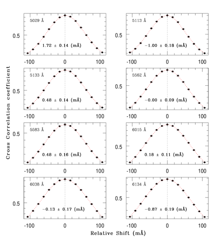
Figure 1: The points with error-bars are the cross-correlation coefficients plotted as a function of the relative shift between UVES and HARPS Th-Ar spectra. The cross-correlation is performed using groups of five consecutive unblended emission lines in the vicinity of the different metal absorption lines of the $z_{\rm abs}$ = 1.1508 system. The observed wavelength of the region around the metal line is given in the top left corner in each panel. The dotted line is the best Gaussian fit to these coefficients. This is used to derive the relative shift between the two spectra with sub-pixel accuracy. The mean relative shift and 1$\sigma$ error as well as the central wavelength of the region used are given in each panel.

To derive the global trend of the relative shift, we have extended our cross-correlation analysis, to the entire wavelength range.

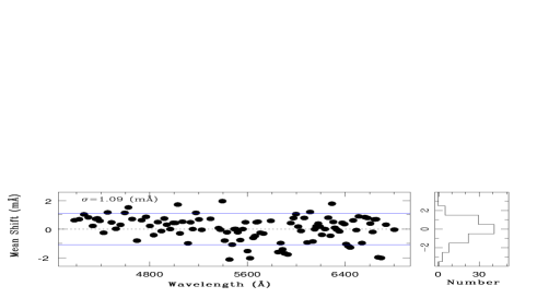
Figure 2: The left panel shows the shift between HARPS and UVES lamp spectra derived by performing the cross-correlation (as shown in Fig. 1) over the wavelength regions consisting of five consecutive unblended Th-Ar lines. The histogram of the mean shift is shown in the right panel. The mean shift is 0.01 mÅ  and the rms $\sigma$ = 1.09 mÅ.

The result of the analysis is shown in Fig. 2. The shifts are obtained in the same way as in Fig. 1. The average of the mean relative shifts over the entire wavelength range is 0.01 mÅ  with an rms deviation of 1.09 mÅ. In what follows we investigate the absolute wavelength calibration accuracies of the two instruments.

3.2 Testing absolute wavelength calibration error of UVES and HARPS

To test the absolute wavelength calibration accuracy we compare the central wavelength of strong un-blended emission lines in the extracted Th-Ar lamp spectrum with the wavelengths tabulated in Cuyper et al. (1998). We model the emission lines by a single Gaussian function. The best-fit line-centroid along with other parameters of the models and errors are determined by a $\chi^{2}$ minimization procedure. In many cases we find it difficult to fit the lines with reduced $\chi^{2}\approx 1$.

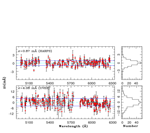
Figure 3: $\Delta\lambda$, the offset of the centroid wavelength of the emission lines in the Th-Ar lamp spectra (obtained using Gaussian fits) with respect to the wavelengths given by Cuyper et al. (1998) is plotted versus wavelength. The left-hand side upper and lower panels show the results for the HARPS and UVES spectra respectively. The corresponding right-hand side panels provide histograms. The root mean square deviation of $\Delta\lambda$ around zero ($\sigma$) is stated explicitly.

In such cases we have scaled the flux errors by square root of the reduced $\chi^{2}$ and re-run the fitting procedure. In this way, we have avoided any underestimation of the errors on the best fit parameters, assuming that the actual errors on the flux of the Th-Ar lamp spectrum was somehow underestimated.

The difference between the best-fit line centroid, in the extracted lamp spectra and the wavelength quoted by Cuyper et al. (1998) is plotted in Fig. 3. The wavelength range shown in this figure is the one covered by the main Fe ii and Mg ii lines of the $z_{\rm abs}$ = 1.1508 system. We find the rms of the deviation ($\Delta\lambda$ in Fig. 3) around zero to be, respectively, 0.87 mÅ  and 4.08 mÅ  for the HARPS and UVES lamp spectra. This clearly demonstrates that the shifts between the HARPS and the UVES lamp spectra measured from the cross-correlation analysis (i.e $\leq 1$ mÅ) are well within the wavelength calibration accuracy of UVES.

In addition, we have used the best-fit FWHM of the Gaussian fit of the lamp lines to derive the spectral resolution ($R=\lambda/FWHM$) of the spectrum. The resolution measurements are shown in Fig. 4. The mean resolution and standard deviation for HARPS and UVES are found to be $R=112,200$ and $\sigma=8,400$; $R=55,100$ and $\sigma=7,600$ respectively.

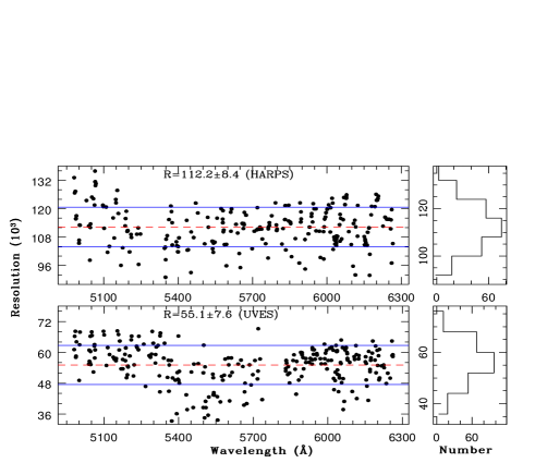
Figure 4: The spectral resolution ($R=\lambda/FWHM$) measured from Gaussian fitting of emission lines in the Th-Ar lamp spectra is plotted versus wavelength. The left-hand side upper and lower panels show the result from HARPS and UVES spectra respectively. The corresponding histograms are shown in the right-hand side panels. The mean along with the standard deviation are stated explicitly.

3.3 Effect of calibration error on $\Delta\alpha/\alpha$ measurement

Next we investigate how the scatter in wavelength calibration ($\Delta\lambda$) translates into a scatter in $\Delta\alpha/\alpha$ . We follow the method used by Murphy et al. (2003) for this purpose. We randomly choose 3 emission lines in the lamp spectrum, with a rest wavelength close to each of the observed wavelengths of the Fe ii and Mg ii lines used in the analysis of the variation of $\alpha$. There are two Mg ii lines, $\lambda$2796 and $\lambda$2803, and five Fe ii lines, $\lambda$2344, $\lambda$2374, $\lambda$2382, $\lambda$2586, and $\lambda$2600. Thus we have 21 ($7\times 3$) lines per realization. By choosing 3 lines, we mimic 3 distinct components in the actual absorption system. We assume that the measured shift in the emission line centroid away from the actual value is caused by the variation in $\alpha$. To estimate this variation, we use the analytic fitting function given by Dzuba et al. (2002),

$$w=w_{o}+qx.$$ (1)

Here, $w_{o}$ and $w$ are, respectively, the vacuum wave number (in units of cm^-1) measured in the laboratory and the modified wave number due to a change in $\alpha$; $x=(\Delta\alpha/\alpha+1)^{2}-1$ and $q$ is the sensitivity coefficient. At each chosen lamp emission line we assign the $q$ value of the neighboring metal absorption transition.

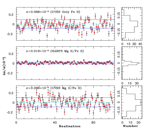
Figure 5: Inferred $\Delta\alpha/\alpha$ due to uncertainties in the wavelength calibration. The results presented in the middle and bottom panels are when we consider 5 main Fe ii lines along with the Mg ii doublet in our analysis. For each realization a set of 21 Th-Ar lines are randomly chosen (3 in the neighborhood of each 5 Fe ii and 2 Mg ii lines of the $z_{\rm abs}$ =1.1508 system). $\Delta\alpha/\alpha$ is computed from the measured deviations in the line centroid by assigning the $q$ coefficient (Dzuba et al. 2002) of neighboring metal line to the Th-Ar emission line. The left-hand side middle and lower panels show the result for the HARPS and UVES spectra respectively. The histogram for both cases are shown in the right-hand side panels. The top panels gives the results for the UVES data when we consider 6 Fe ii lines (i.e Fe ii$\lambda 1608$ and 5 main Fe ii lines) in the analysis. The $\sigma$ of the distribution refers to a typical error on the measurement of $\Delta\alpha/\alpha$ due to wavelength calibration alone in a single system with 3 distinct components.

All the lamp emission lines in each realization are fitted simultaneously with Gaussians, for one fixed value of $\Delta\alpha/\alpha$ . Here, the $\Delta\alpha/\alpha$ value is used to modify the rest wavelength of the emission lines using the $q$ coefficients given by Dzuba et al. (2002) for the corresponding metal lines. This procedure is repeated for a range of $\Delta\alpha/\alpha$ , from $-2.0\times 10^{-5}$ to $2.0\times 10^{-5}$ in steps of $0.02\times 10^{-5}$ to achieve $\chi^{2}$ as a function of $\Delta\alpha/\alpha$ . The $\chi^{2}$ versus $\Delta\alpha/\alpha$ curve is used to extract the best fitted $\Delta\alpha/\alpha$ (with error-bars) in a similar way as is used in the absorption system (discussed in the next Section). The measured spurious $\Delta\alpha/\alpha$ for 100 random realizations are plotted in Fig. 5 both for HARPS (left-hand side middle panel) and UVES (left-hand side lower panel) lamp spectra. In the top panel we give the results for similar analysis of UVES spectrum considering 6 Fe ii lines (i.e including Fe ii$\lambda$1608 instead of Mg ii doublet) alone.

We notice that the measured values of $\Delta\alpha/\alpha$ obtained in this experiment have a Gaussian-shape distribution with $\sigma$ of $0.02\times 10^{-5}$ for HARPS and $\sigma\simeq 0.1\times 10^{-5}$ for UVES. As the system under consideration is known to have much more than 3 components, the above quoted values are conservative errors due to uncertainties in the wavelength calibration. Murphy et al. (2003) have also carried out such analysis for HIRES Th-Ar lamp spectra. Their weighted mean from the sample of 128 sets of Th-Ar lines resulted in $\langle\Delta\alpha/\alpha\rangle_{ThAr}=(0.4\pm 0.8)\times 10^{-7}$. If one assumes a Gaussian distribution for the individual values, then the central limits theorem implies that the typical $\sigma$ from one set of Th-Ar lines in the case of HIRES should be around $0.09\times 10^{-5}$ ($\equiv 0.8\times 10^{-7}\times\sqrt{128}$), which is similar to our value for UVES Th-Ar lamp spectra (i.e $\sigma=0.1\times 10^{-5}$).

3.4 Effect of using different Th-Ar line tables on wavelength calibration

Th-Ar reference wavelengths are taken from the compilations of Palmer et al. (1983) for Thorium lines and Norlén et al. (1973) for Argon lines. The line lists built from these compilations and commonly used for echelle spectroscopy calibration are available on the web-pages of the European Southern Observatory (ESO) and the National Optical Astronomy Observatory (NOAO). The two tables differ slightly, because the ESO Th-Ar line table is not accurate up to 4 decimal places as is the case with NOAO Th-Ar line table.

Figure 6: The difference, $\delta\lambda_{fit}$, between the best-fit centroid of Th-Ar lines seen in the UVES Th-Ar lamp spectrum and their wavelength listed in the NOAO Th-Ar table is plotted versus the difference between the corresponding wavelengths listed in the ESO and NOAO Th-Ar line tables ($\Delta\lambda_{tab}$). The figure shows that (i) the scatter of $\Delta\lambda_{tab}$ is about a factor 3 smaller than that of $\delta\lambda_{fit}$ (ii) no clear correlation is seen between $\Delta\lambda_{tab}$ and $\delta\lambda_{fit}$. As a result the calibration errors due to differences in wavelengths given in different Th-Ar tables is negligible as compare to the wavelength calibration accuracy of the instrument.

For the extraction of UVES lamp spectra we have used the Th-Ar line table provided by NOAO. To investigate whether the use of ESO table could induce systematic shifts in $\Delta\alpha/\alpha$ , we have also extracted the same UVES Th-Ar lamp spectrum using the Th-Ar line table provided by ESO. We fit a Gaussian function to the un-blended Th-Ar line as described in sub-section 3.2 and get the deviation, $\delta\lambda_{fit}$, of the best-fit centroid with respect to the corresponding value in the NOAO Th-Ar table. The deviation ($\delta\lambda_{fit}$) is plotted in Fig. 6 as a function of the difference in the wavelengths tabulated by ESO and NOAO, $\Delta\lambda_{tab}$. If the wavelength uncertainties caused by the inaccurate wavelengths listed in ESO Th-Ar table for some of the Th-Ar lines are larger than the errors allowed by the dispersion solution, then we expect a correlation between $\delta\lambda_{fit}$ and $\Delta\lambda_{tab}$. The lack of such a correlation and the larger scatter of $\delta\lambda_{fit}$ compared to $\Delta\lambda_{tab}$ in the figure, show that the effect of inaccurate rest-wavelengths of a few lines in the ESO line list is negligible.

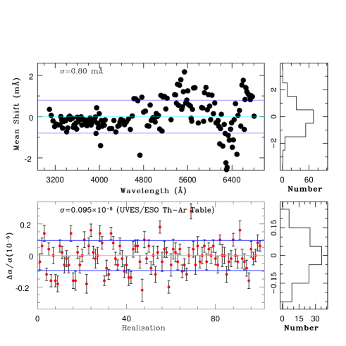
Figure 7: The figure shows the effect of calibration using two different Th-Ar line tables: (i) provided by NOAO and usually used in IRAF (ii) provided by ESO and used in MIDAS. The upper left panel shows the mean shift of Th-Ar lamp spectrum calibrated using ESO Th-Ar line table with respect to the same Th-Ar lamp spectra but calibrated using the NOAO Th-Ar line table. The mean shift is derived by performing the cross-correlation as is shown in Fig. 1 over a wavelength region consisting of about 5 consecutive unblended Th-Ar lines. The histogram of the mean shift is shown in the right panel. The lower left panel shows the similar plot as in the lower left panel of Fig. 5, except that here Th-Ar lamp spectrum is calibrated using the ESO Th-Ar lines table rather than the NOAO Th-Ar lines table. The bottom right panel shows the histogram of the $\Delta\alpha/\alpha$ values.

To complement this, we perform the cross-correlation between the lamp spectra calibrated using the two wavelength tables. The cross-correlation is performed in a similar way as described in sub-section 3.1. Here we have shifted the UVES lamp spectrum calibrated using the ESO Th-Ar table over the same lamp spectrum calibrated using the NOAO Th-Ar line table. The result of the cross-correlation is shown in the upper panel of Fig. 7. From the figure it can be seen that the relative shift is not completely random. However the relative shift is most of the time less than 2mÅ and even 1mÅ, which is well within the UVES calibration accuracy.

We also repeat the exercise to derive how these wavelength calibration uncertainties translate into $\Delta\alpha/\alpha$ as described in detail in sub-section 3.3 for the case when one uses for calibration the ESO Th-Ar line table (Fig. 5 for UVES lamp uses NOAO table). The result is shown in the lower left-hand side panel of the Fig. 7 for 100 realizations. The histogram shown in the lower right-hand side panel shows that the fiducial $\Delta\alpha/\alpha$ is distributed like a Gaussian. As a result, we can conclude that the $\Delta\alpha/\alpha$ measurements in the literature (Chand et al. 2004 & 2005, Quast et al. 2004) using the ESO Th-Ar line table, should not be significantly affected by this possible systematic effect.

4 Analysis

In this section we present the results on the measurement of $\Delta\alpha/\alpha$ using the HARPS and UVES spectra. The details of the analysis used here, validation of the procedure using simulated spectra and the error budget from $\chi^{2}$ analysis can be found in Chand et al. (2004, 2005). Here, we mainly concentrate on (i) comparing the methods used by Chand et al. (2004, 2005) to derive $\Delta\alpha/\alpha$ with that used by Quast et al. (2004) and (ii) understanding the effect of the decomposition of the absorption profiles into multiple narrow Voigt-profile.

4.1 Re-analysis of the red sub-system in the UVES data

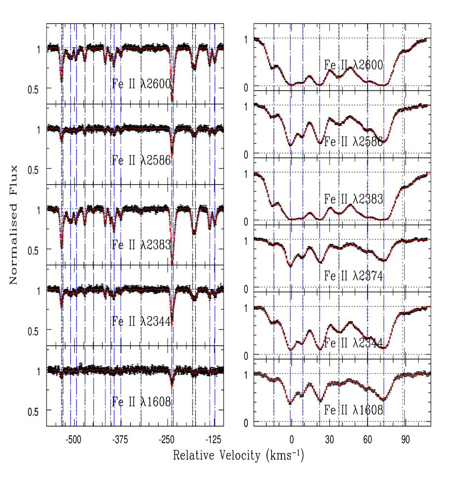
Figure 8: The figure shows the velocity plot of observed profiles (data points with error-bars) together with the best fitted Voigt-profile for $\Delta\alpha/\alpha$ $=0$ over plotted as a solid curve, to the blue (left-hand side panels) and red-subsystem (right-hand side panels) of the $z_{\rm abs}$ =1.1508 in the UVES spectrum. The dotted and dashed vertical lines are respectively the locations of the individual components obtained in this study and that of Quast et al. (2004).

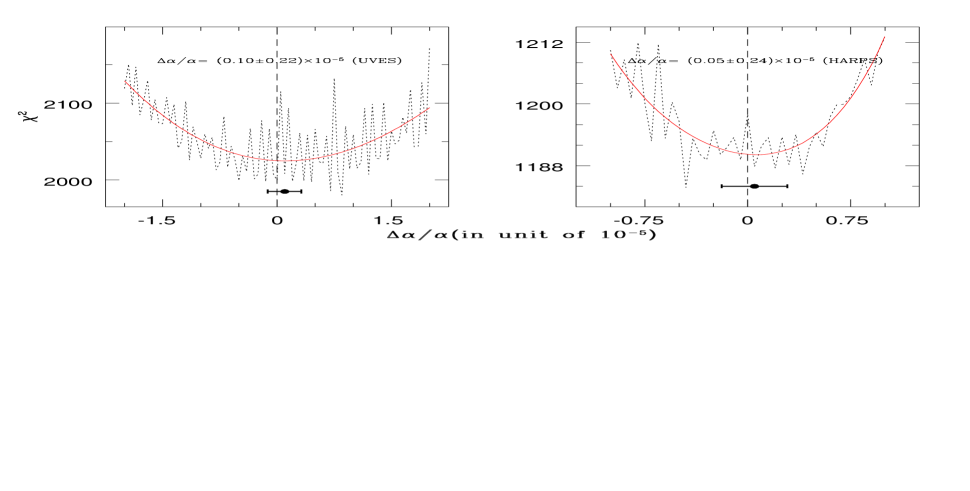
Figure 9: The dotted curve in both the panels indicates the variations of $\chi^{2}$ as a function of $\Delta\alpha/\alpha$ as measured using the UVES (left panel) and HARPS (right panel) spectra. The solid curve are the polynomial fit to these curve obtain using rms minimization to avoid local fluctuations. Dark rectangles with error bar indicate the position of the minimum with one sigma error-bar obtained from $\chi^{2}_{min}+1$ statistics. The $\chi^{2}$ curve in the left-hand side panel is derived based on the initial fit of UVES data shown in Fig. 8, while the curve in the right-hand side panel is obtained by using simultaneously the initial fit of HARPS data shown in Fig. 12 and Fig. 13.

In the analysis of Chand et al (2004, 2005) $\Delta\alpha/\alpha$ is not explicitly used as fitting parameter. Instead $\chi^{2}$ versus $\Delta\alpha/\alpha$ curve is used to get the best fitted value of $\Delta\alpha/\alpha$ . However, Quast et al. (2004) use the Voigt profile analysis keeping $\Delta\alpha/\alpha$ also as a fitting parameter in addition to $N$, $b$ and $z$. Chand et al. (2005), using analytic calculations, have shown that both the approaches should give the same result. Here we check this by re-analysing the absorption lines of the $z_{\rm abs}$ = 1.1508 system toward HE 0515$-$4414 using $\chi^{2}$ versus $\Delta\alpha/\alpha$ curve.

The absorption lines of this system is spread over about 730 km s^-1 (Quast et al. 2004). We have divided the whole system in two well detached blue and red sub-systems. The blue sub-system covers the velocity range $-$570 to $-$100 km s^-1 and the red sub-system covers the velocity range $-$20 to $+$110 km s^-1 with respect to $z_{\rm abs}$=1.1508. Our best fit Voigt-profiles to the blue and red sub-system using the UVES spectrum, is shown respectively in the left and right-hand side panels of Fig. 8. The vertical dotted lines are best fitted velocity components obtained in this study and the long dashed vertical lines mark the velocity components of the Quast et al. (2004). Apart form the component around $\sim 90$ km s^-1 , we find almost perfect matching between the components obtained with two different fitting codes. The variation of $\chi^{2}$ as a function of $\Delta\alpha/\alpha$ using this initial fit (Fig. 8) is shown in the left-hand side panel of Fig. 9. The scatter seen in the $\chi^{2}$ curve is mainly due to low column density of many components in blue sub-system (see the discussion in Chand et al. 2004). The position of the minimum in the $\chi^{2}$ curve remains uncertain till either we smooth the curve or fit some smoothing polynomial to it. Therefore we have fitted a polynomial function of 4th order minimizing the rms deviation. The best fit of the $\chi^{2}$ curve is shown by the solid line (left-hand side panel of Fig. 9). Its minimum gives $\Delta\alpha/\alpha$  = ${(0.10\pm 0.22)\times 10^{-5}}$, using $\chi^{2}_{min}+1$ statistics. The derived position of the minimum does not depart significantly when we use a 2nd or 3rd order polynomial fit to the $\chi^{2}$ data points. Our best fitted value, $\Delta\alpha/\alpha$ = ${(0.10\pm 0.22)\times 10^{-5}}$, is very much consistent with that obtained by Quast et al. (2004) ($\Delta\alpha/\alpha$  = ${[0.01\pm 0.17]\times 10^{-5}}$).

Figure 10: Comparison of parameters derived for individual components from the fit of the UVES spectrum in this study and that of Quast et al. (2004).

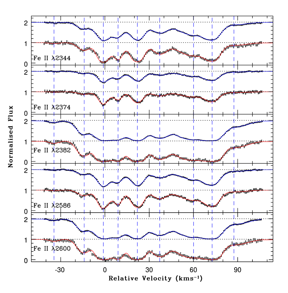
Figure 11: Absorption profiles in the red sub-system of the $z_{\rm abs}$ = 1.1508 DLA toward HE 0515$-$4414 as observed with HARPS and UVES plotted on a velocity scale. The normalized UVES spectrum is shifted in the y-direction by one unit for the sake of clarity. The data points with error-bars correspond to the observed spectra. Over plotted as a solid curve is the best Voigt-profile fit based on the UVES data alone (same as in right-hand side panels of Fig. 8). For HARPS data the fit based on UVES data has been convolved with HARPS instrumental profile. The figure demonstrates the requirement for extra components, as evident from the higher spectral resolution HARPS spectrum (see for example region around $-$20 to 30  $kms^{-1}$).

The best fitted column densities and Doppler parameters in individual components also agree well (see Fig. 10).

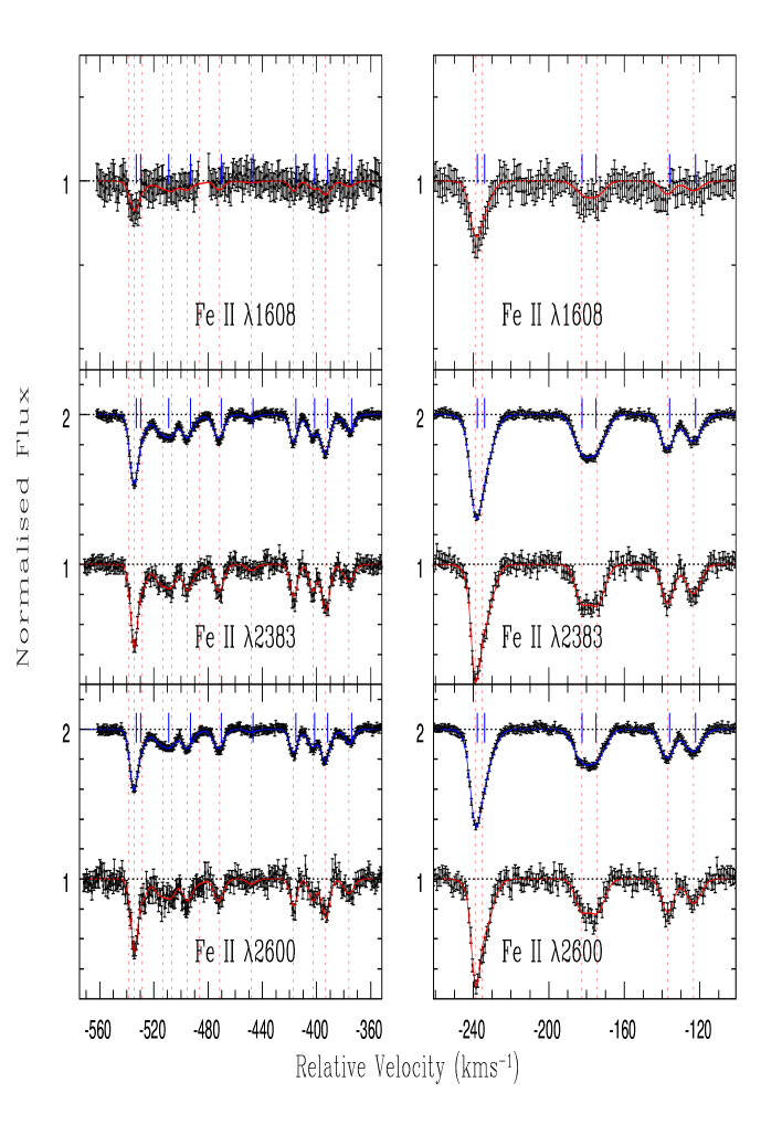
Figure 12: Absorption profiles in the blue sub-system of the $z_{\rm abs}$ =1.1508 on a velocity scale. The normalized UVES spectrum is shifted by unity for better visualization. The data points with error-bars correspond to the observed spectra. Over plotted as solid curves are the best Voigt-profile fits at $\Delta\alpha/\alpha$ $=0$. The Voigt-profile fits of both the HARPS and UVES data, shown here are based on the component structure derived by imposing the condition that the HARPS ($R=112000$) as well as the UVES ($R=55,000$ and better S/N) data should be fitted with parameters that are consistent with each others. The dotted vertical lines mark the positions of components required to fit the HARPS data. The thick ticks mark the position of components as is derived using the UVES data alone (Fig. 8)

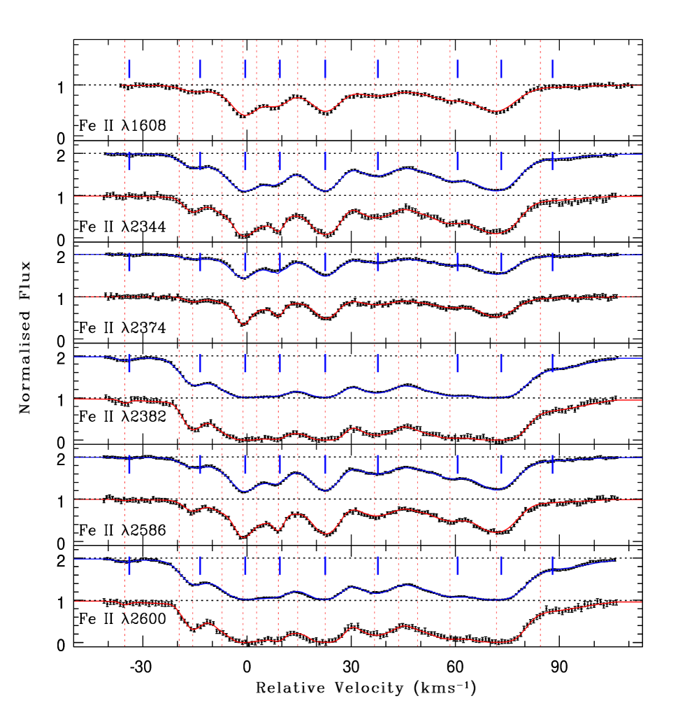
Figure 13: Same as Fig. 12 for the red sub-system. In addition, the figure also illustrate more clearly that the HARPS data require more components (15 components, shown by dotted line) compared to the UVES data alone (9 components, shown by thick ticks). Also note that the fit shown for the UVES data is based on the component structure obtained in conjunction to HARPS data. For comparison the component required to fit the UVES data alone (from Fig. 8 right-hand side panels) are marked by thick tick.

Table 1: Results of the Voigt profile fit of Fe ii lines at $z_{\rm abs}$= 1.1508 toward HE 0515$-$4414.

C.N	$z_{\rm abs}$	b	log[N(Fe ii)]	Va
		(km s-1 )	(cm-2)	(km s-1 )
1	$1.146938\pm 0.00000^{\dagger}$	$1.70\pm 0.22$	$11.38\pm 0.14$	$-538.79\pm 00.00$
2	$1.146969\pm 0.000098$	$2.34\pm 0.25$	$12.30\pm 0.03$	$-534.46\pm 13.71$
3	$1.147008\pm 0.00000^{\dagger}$	$4.47\pm 0.75$	$11.90\pm 0.06$	$-529.02\pm 00.00$
4	$1.147117\pm 0.001030$	$7.45\pm 1.01$	$12.01\pm 0.04$	$-513.80\pm 143.7$
5	$1.147169\pm 0.000410$	$4.25\pm 0.88$	$11.58\pm 0.09$	$-506.54\pm 57.27$
6	$1.147249\pm 0.000106$	$4.63\pm 0.22$	$11.92\pm 0.04$	$-495.37\pm 14.83$
7	$1.147312\pm 0.00000^{\dagger}$	$4.90\pm 0.45$	$11.23\pm 0.17$	$-486.57\pm 00.00$
8	$1.147416\pm 0.000096$	$4.70\pm 0.19$	$11.93\pm 0.04$	$-472.05\pm 13.33$
9	$1.147587\pm 0.000255$	$4.49\pm 0.67$	$11.24\pm 0.15$	$-448.18\pm 35.65$
10	$1.147809\pm 0.000113$	$3.47\pm 0.22$	$11.91\pm 0.04$	$-417.19\pm 15.84$
11	$1.147911\pm 0.000133$	$3.39\pm 0.25$	$11.81\pm 0.04$	$-402.96\pm 18.58$
12	$1.147980\pm 0.000215$	$3.75\pm 0.57$	$12.12\pm 0.10$	$-393.33\pm 30.04$
13	$1.148101\pm 0.000543$	$4.99\pm 1.12$	$11.75\pm 0.07$	$-376.44\pm 75.84$
14	$1.148501\pm 0.000218$	$7.52\pm 0.44$	$11.56\pm 0.10$	$-320.62\pm 30.47$
15	$1.148783\pm 0.000287$	$2.97\pm 0.57$	$11.09\pm 0.18$	$-281.27\pm 40.03$
16	$1.149088\pm 0.000096$	$2.11\pm 0.21$	$12.44\pm 0.03$	$-238.72\pm 13.32$
17	$1.149112\pm 0.000057$	$6.46\pm 0.11$	$12.52\pm 0.03$	$-235.38\pm 07.97$
18	$1.149489\pm 0.000398$	$4.30\pm 0.43$	$12.03\pm 0.03$	$-182.79\pm 55.50$
19	$1.149547\pm 0.000470$	$5.50\pm 0.53$	$12.20\pm 0.02$	$-174.70\pm 65.55$
20	$1.149817\pm 0.000061$	$4.14\pm 0.12$	$12.08\pm 0.03$	$-137.05\pm 08.56$
21	$1.149915\pm 0.000108$	$5.12\pm 0.21$	$12.01\pm 0.03$	$-123.38\pm 15.02$
22	$1.150548\pm 0.00000^{\dagger}$	$0.26\pm 0.0^{\ddagger}$	$11.21\pm 0.16$	$-35.13\pm 00.00$
23	$1.150659\pm 0.00000^{\dagger}$	$17.85\pm 0.0^{\ddagger}$	$12.21\pm 0.06$	$-19.65\pm 00.00$
24	$1.150688\pm 0.000107$	$2.98\pm 0.18$	$12.58\pm 0.02$	$-15.61\pm 14.94$
25	$1.150747\pm 0.00000^{\dagger}$	$4.62\pm 0.78$	$12.47\pm 0.32$	$-7.39\pm 00.00$
26	$1.150792\pm 0.000102$	$1.95\pm 0.18$	$13.26\pm 0.03$	$-1.11\pm 14.20$
27	$1.150819\pm 0.00000^{\dagger}$	$8.16\pm 1.67$	$13.46\pm 0.07$	$2.65\pm 00.00$
28	$1.150864\pm 0.000126$	$1.07\pm 0.25$	$12.88\pm 0.05$	$8.92\pm 17.53$
29	$1.150903\pm 0.00000^{\dagger}$	$3.65\pm 2.03$	$12.58\pm 0.37$	$14.36\pm 00.00$
30	$1.150962\pm 0.000190$	$4.21\pm 0.21$	$13.47\pm 0.03$	$22.58\pm 26.50$
31	$1.151063\pm 0.000207$	$6.68\pm 0.39$	$13.09\pm 0.02$	$36.66\pm 28.89$
32	$1.151113\pm 0.00000^{\dagger}$	$6.00\pm 1.61$	$12.34\pm 0.11$	$43.63\pm 00.00$
33	$1.151152\pm 0.00000^{\dagger}$	$3.37\pm 0.83$	$12.25\pm 0.08$	$49.06\pm 00.00$
34	$1.151218\pm 0.000235$	$7.13\pm 0.38$	$13.29\pm 0.02$	$58.26\pm 32.68$
35	$1.151314\pm 0.000158$	$6.21\pm 0.17$	$13.56\pm 0.02$	$71.64\pm 22.06$
36	$1.151406\pm 0.00000^{\dagger}$	$15.40\pm 0.0^{\ddagger}$	$12.72\pm 0.02$	$84.46\pm 00.00$
‘a’ relative velocity with respect to $z_{\rm abs}=1.1508$.
‘†’ The redshift ($z$) of these components are kept fixed.
‘‡’ The Doppler parameter, $b$, of these components are kept fixed.

The larger errors in the measured quantities in the present study is mainly due to higher values of the error assigned to the flux in individual pixels. Thus the analysis presented here clearly shows that the analysis used by us in Chand et al (2004, 2005) produces consistent results.

In addition we have also performed the analysis of UVES spectra by excluding the weaker Fe ii lines from the blue sub-system and heavily saturated strong Fe ii$\lambda\lambda$2383,2600 lines from the red-subsystem, (see discussion in Chand et al. 2004). In this case the $\chi^{2}$ curve is found relatively less fluctuating as compare to the left-hand side panel of Fig. 9, and has resulted in $\Delta\alpha/\alpha$ = $(0.00\pm 0.26)\times 10^{-5}$.

4.2 $\Delta\alpha/\alpha$ from the HARPS data

The decomposition of the absorption profiles in sub-components is expected to be better defined from the HARPS spectrum because of its superior spectral resolution. In Fig. 11 we compare the profiles of the Fe ii lines in the red sub-system as observed with HARPS and UVES. The best multi-component Voigt-profiles fit using the UVES spectrum alone is over plotted. To fit the HARPS data we need additional components, as is apparent in the region around $-$20 to $+$30 km s^-1 where consistent differences are seen for all profiles between the HARPS spectrum and the fit to the UVES data alone. However, the UVES spectrum has the advantage of having higher S/N. Thus, in our analysis we fitted simultaneously both HARPS and UVES data using the same component structure and the appropriate instrumental functions. We initially fitted the HARPS data and used the derived parameters to fit the UVES data. The process was repeated until the residuals along the profiles are symmetrically distributed around zero and the best-fit parameters from these two data sets are consistent with one another within measurement uncertainties. In this exercise we have not included the line Fe ii$\lambda$1608 (covered only in the UVES spectrum) so that our derived component structure is not artificially bias towards $\Delta\alpha/\alpha$ $=0$.

Our best-fit Voigt-profile components that simultaneously fit the HARPS and UVES spectra are shown in Fig. 12,13 respectively for the blue and red sub-systems. The best-fit parameters are listed in Table. LABEL:model.tab. The component identification number (C.N), redshift ($z$), velocity dispersion ($b$), and Fe ii column density ($N$), for each component are listed respectively in columns 1, 2, 3 and 4. The last column of the table lists the relative velocity of the components with respect to $z_{\rm abs}$=1.1508. We find that the blue and red sub-system (Fig. 12,13) require respectively 3 and 6 extra components compared to the minimum number required to fit the UVES spectrum alone with $\chi^{2}=1$.

We evaluate the best-fit $\Delta\alpha/\alpha$ value using the high resolution HARPS spectrum for the five main Fe ii lines and the UVES spectrum for Fe ii$\lambda 1608$ considering both the blue and red sub-systems simultaneously. Here it should be noted that the Fe ii$\lambda$1608 is crucial for $\Delta\alpha/\alpha$ measurement due to its opposite sensitivity for $\Delta\alpha/\alpha$ (negative $q$ coefficient) compared to the other main Fe ii lines. However as its observed wavelength range ($\approx 3460$Å) is not covered by the HARPS spectral coverage (3800 - 6900Å), we have to use it from the UVES spectrum for constraining the $\Delta\alpha/\alpha$ value. The $\chi^{2}$ versus $\Delta\alpha/\alpha$ curve is shown in the right-hand side panel of Fig. 9. The scatter seen in the $\chi^{2}$ curve is mainly due to the low S/N ratio and low column density of many components as can be seen from Table LABEL:model.tab (see the discussion in Chand et al. 2004). The continuous curve gives the 4th order polynomial fit to the $\chi^{2}$ data points using rms minimisation. Its minimum gives $\Delta\alpha/\alpha$  = ${(0.05\pm 0.24)\times 10^{-5}}$, using $\chi^{2}_{min}+1$ statistics. This result is consistent with the Quast et al. (2004) measurement ($\Delta\alpha/\alpha$  = ${[0.01\pm 0.17]\times 10^{-5}}$) based on the UVES spectrum and lesser number of components. Thus in this particular case lack of information on the additional components in the UVES spectrum does not seem to affect the final result.

5 Result and discussion

In this paper, we present a very high resolution (R = 112,000) spectrum of QSO HE 0515$-$4414 obtained using HARPS. We have used the high wavelength calibration accuracy and high spectral resolution capabilities of HARPS to address the following issues.

We compare the lamp spectra obtained with UVES and HARPS. Using cross-correlation analysis we show that any possible relative shift between the two spectra are within 2 mÅ. Using Gaussian fits to unblended lamp emission lines, we find that the absolute wavelength calibration of HARPS is very robust with rms deviation of 0.87 mÅ with respect to the wavelengths tabulated in Cuyper et al. (1998). This is about a factor of 4 better than that of UVES ($\sigma=4.08$ mÅ, see Fig. 3). Thus the small shifts noted between the HARPS and UVES lamp spectra are well within the typical wavelength calibration accuracy of UVES. We have derived the error on $\Delta\alpha/\alpha$ measurements due to the calibration accuracy alone. For UVES and HARPS spectra this is found to be respectively $\sigma=0.96\times 10^{-6}$ and $\sigma=0.19\times 10^{-6}$ for a typical system with three well detached components. The value obtained for the UVES spectrum is also consistent with that of HIRES (Murphy et al. 2003).

This shows that HARPS is the ideal instrument for this kind of measurement. Unfortunately it is mounted on the 3.6 m telescope at La Silla and only HE 0515$-$4414 is bright enough to be observed in a reasonable amount of time. This shows as well that the UVES spectra reduced (or calibrated) with the UVES pipeline and used in the literature to constrain $\Delta\alpha/\alpha$ (Srianand et al. 2004 and Chand et al. 2004, Quast et al. 2004, Chand et al. 2005) do not suffer from major systematic error in the wavelength calibration.

We have obtained the accurate multi-component structure using the higher resolution data (R $\approx 112,000$ for HARPS compared to $\approx 55,000$ for UVES). The best fit to the profiles obtained by fitting simultaneously the HARPS data (of higher resolution) and the UVES data (of better S/N ratio) require additional components as compared to the fit using the UVES data alone (Quast et al. 2004). Using this new sub-component decomposition and both HARPS and UVES data, we find $\Delta\alpha/\alpha$  $=(0.05\pm 0.24)\times 10^{-5}$. This is consistent with the results derived by Quast et al. (2004) from the UVES data alone. Indeed, we have in addition re-analyzed the UVES data which was used in Quast et al. (2004) (without using the component structure from HARPS data), to estimate the effect of different independent algorithms used to obtain error spectra, to combine the data, to fit the continuum and to fit the absorption lines. We find that the best-fit parameters as well as the $\Delta\alpha/\alpha$ measurement ($\Delta\alpha/\alpha$  = ${[0.10\pm 0.22]\times 10^{-5}}$), obtained by our independent analysis, are consistent with that of Quast et al. (2004) ($\Delta\alpha/\alpha$  = ${[0.01\pm 0.17]\times 10^{-5}}$).

We note that the precision on the $\Delta\alpha/\alpha$ measurement obtained using the HARPS spectrum, which is of high resolution and low S/N ratio, is similar to that obtained from the UVES spectrum, which is of lower resolution and higher S/N ratio. Therefore, the improvement in the wavelength calibration accuracy by an order of magnitude using HARPS will be effective to improve the constrain on $\Delta\alpha/\alpha$ only if high S/N ratio can also be obtained. This could be possible if an instrument such as HARPS can be mounted on bigger telescopes.

References

- (1) Bahcall, J. N., Sargent, W. L. W. & Schmidt, M. 1967, ApJ, 149, L11
- (2) Bahcall, J. N., Steinhardt, C. L., & Schlegel, D. 2004, ApJ, 600, 520
- (3) Chand, H., Srianand, R., Petitjean, P., Aracil, B., 2004, A&A, 417, 853
- (4) Chand, H., Petitjean, P, Srianand, R., Aracil, B., 2005, A&A, 430, 47
- (5) Chengalur, J. N., Kanekar, N., 2003, Phys. Rev. Lett., 91, 241302
- (6) Cowie, L. L., & Songaila, A., 1995, ApJ, 453, 596
- (7) Cuyper, De- J.-P., Hensberge, H., 1998, A&AS, 128, 409
- (8) Darling, J., 2003, Phys. Rev. Lett., 91, 011301
- (9) Darling, J., 2004, ApJ, 612, 58
- (10) De la Varga, A., Reimers, D., Tytler, D., et al. 2000, A&A, 363, 69
- (11) Dzuba, V. A., Flambaum, V. V., Kozlov, M. G. et al. 2002, Phys. Rev A., 66, 022501
- (12) Edlén, B. 1966, Metrologica, 2, 71
- (13) Fischer, M et al., 2004, Phys. Rev. Lett., 92, 230802
- (14) Fujii, Y, et al., 2000, Nucl. Phys. B, 573, 377
- (15) Griesmann U., & Kling, R., 2000, ApJ, 536, L113
- (16) Kanekar, N., Chengalur, J. N., 2004, MNRAS, 350, L17
- (17) Levshakov, S. A. 1994, MNRAS, 269, 339
- (18) Levshakov, S. A., Centurión, M., Molaro, P., D’Odorico, S. A&A 2005a, 434, 827
- (19) Levshakov, S. A., Centurión, M., Molaro, P., D’Odorico, S., Reimers, D., Quast, R., Pollmann, M., 2005b, ArXive Astrophysics e-prints, astro-ph/0511765
- (20) Marion, H., Phys. Rev. Lett., 2003, 90, 150801
- (21) Martinez, A. F., Vladilo, G., & Bonifacio, P. 2003, MSAIS, 3, 252
- (22) Martin, W. C, Zalubas, R., 1983, J. Phys. Chem. Ref. Data, 12, 323
- (23) Mosser, B., Michel, E., Samadi, R. et al. 2004, Messenger, 114, 20
- (24) Murphy, M. T., Webb, J., Flambaum, V., Prochaska, J. X., & Wolfe, A. M. 2001a, MNRAS, 327, 1237
- (25) Murphy, M. T., Webb, J., Flambaum, V., Drinkwater, M. J., Combes, F., Wiklind, T. 2001b, MNRAS, 327, 1244
- (26) Murphy, M. T., Webb, J. K., Flambaum, V. V. 2003, MNRAS, 345, 609
- (27) Norlén, G., 1973, Physica Scripta, 8, 249
- (28) Palmer, B. A. and Engleman, R., Jr., 1983, Atlas of the Thorium Spectrum, Los Alamos National Laboratory
- (29) Petitjean, P., & Aracil, B. 2004, A&A, 422, 523
- (30) Petitjean, P., Ivanchik, A., Srianand, R., et al., 2004, C. R. Physique, 5, 411
- (31) Potekhin, A. Y., & Varshalovich, D. A. 1994, A&AS, 104, 89
- (32) Quast, R., Reimers, D., & Levshakov, S. A. 2004, A&A, 415, L7
- (33) Quast, R., Reimers, D., Smette, A. et al. 2005, Proceedings of the 22nd Texas Symposium on Relativistic Astrophysics at Stanford University, page 1416
- (34) Srianand, R., Chand, H., Petitjean, P., Aracil, B., 2004, Phys. Rev. Lett., 92, 121302
- (35) Tzanavaris, P., Webb, J. K., Murphy, M. T., Flambaum, V. V., Curran, S. J., 2005, Phys. Rev. Lett., 95, 041301
- (36) Uzan, J.-P, 2003, RvMP, 75, 403
- (37) Uzan, J.-P, 2004, ArXive Astrophysics e-prints, astro-ph/0409424
- (38) Varshalovich, D. A., Panchuk, V. E. & Ivanchik, A. V. 1996, Astron. Lett., 22, 6
- (39) Varshalovich, D. A., Potkhin, A. Y. & Ivanchik, A. V. 2000, in Dunford R. W., Gemmel D.S., Kanter E. P., Kraessig B., Southworth S. H., Yong L., eds, AA Conf. Proc. 506, X-ray and Inner-shell Processes. Argonne National Laboratory, Argonne, IL, 503
- (40) Webb, J. K., Murphy, M. T., Flambaum, V. V., Dzuba V. A., Barrow J. D., Churchill C. W., Prochaska J. X., Wolfe A. M., 2001, Phys. Rev. Lett., 87, 091301
- (41) Wolfe, A. M., Brown, R. L., & Roberts, M. S. 1976, Phys. Rev. Lett., 37, 177