The early reionization with the primordial magnetic fields

Abstract

The early reionization of the intergalactic medium, which is favored from the WMAP temperature-polarization cross-correlations, contests the validity of the standard scenario of structure formation in the cold dark matter cosmogony. It is difficult to achieve early enough star formation without rather extreme assumptions such as very high escape fraction of ionizing photons from proto-galaxies or a top-heavy initial mass function. Here we propose an alternative scenario that is additional fluctuations on small scales induced by primordial magnetic fields trigger the early structure formation. We found that ionizing photons from Population III stars formed in dark haloes can easily reionize the universe by $z\simeq 15$ if the strength of primordial magnetic fields is between $0.7$–$1.5\times 10^{-9}$ Gauss.

1 introduction

The reionization process of the intergalactic medium (IGM) is one of the major remaining problems in modern cosmology. From the Gunn-Peterson test of QSO absorption lines, it is known that the vast majority of IGM is ionized by $z\sim 6$ (Becker et al., 2001; Fan et al., 2002). The recent measurement of the cosmic microwave background (CMB) temperature and polarization cross correlations by WMAP implies that the optical depth of the universe is about $0.17$ (Spergel et al., 2003; Kogut et al., 2003). This result favors the early reionization scenario: the reionization process occurs at $z=15$ – $20$ and the reionization sources are first stars, unlike quasars and galaxies which are known as the reionization sources previously (for the details see Loeb & Barkana 2001).

The early reionization process by the stellar sources has been studied in detail after WMAP (Cen, 2003; Fukugita & Kawasaki, 2003; Ciardi et al., 2003; Somerville & Livio, 2003; Haiman & Holder, 2003). In these works, cold dark matter cosmogony with WMAP parameters is employed. What they found was it is difficult to get $\tau=0.17$ if the standard Salpeter initial mass function (IMF) is adapted. To have early enough reionization, one needs to assume almost $100\%$ escape fraction of ionizing photons from proto-galaxies, or introduce a top-heavy IMF. Heavy stars may form in the early universe induced by the $\rm H_{2}$ molecular cooling while it is still little known about the IMF in the early universe.

An alternative scenario to realize early reionization is to enhance the amplitude of the CDM power spectrum on very small scales. Such enhancement makes the dark haloes form earlier. Accordingly the star formation process starts early enough to achieve $\tau=0.17$. The observational data from redshift surveys of galaxies such as 2dF and SDSS, and Ly-$\alpha$ clouds (Spergel et al., 2003; Seljak et al., 2005) strongly constrain the amplitude of the density fluctuations in the scales larger than 1 Mpc. However, the amplitude in the scales which are relevant to the first star formation, $0.01$ – $0.1$ Mpc, is still unclear. Therefore there is still room for considering additional power in the power spectrum on very small scales. For example, models with initially running spectral index $n>1$ on small scales, additional fluctuations from the isocurvature modes, or non-Gaussian statistics are considered in the context of early reionization (Chen et al., 2003; Avelino & Liddle, 2004; Sugiyama et al., 2004).

If there exist strong enough primordial magnetic fields at the reionization epoch, these magnetic fields produce additional density fluctuations of baryons by the Lorentz force. The magnetic tension is more effective on small scales where the entanglements of magnetic fields are larger. Therefore we expect to have additional power in the density power spectrum on small scales as is the case of isocurvature perturbations. Structure formation by magnetic fields was first discussed by Wasserman (1978). More detailed analysis was carried by Kim et al. (1996) and the influence on the formation of large scale structure was recently estimated by Gopal & Sethi (2003). Sethi & Subramanian (2005) pointed out that nanoGauss magnetic fields can induce early structure formation and may have the potential to achieve the early reionization implied by the WMAP team. They also studied reionization of IGM induced by the dissipation of magnetic energy. In this paper, we thoroughly investigate the role of primordial magnetic fields on the early reionization process. We concentrate on the early structure formation due to the additional power spectrum generated by magnetic fields.

It is known that there exist magnetic fields of several $\mu$Gauss in most of the galaxies and the clusters of galaxies while the origin of these magnetic fields is still uncertain. Coherence lengths of these magnetic fields are typically $100$ kpc –$1$ Mpc (Kronberg, 1994).

Perhaps small seeds of the magnetic fields are produced inside astronomical objects such as stars and AGNs due to the Biermann battery mechanism. Although the resultant magnetic fields are very weak, those may be amplified by the dynamo process (Zeldovich et al. 1983; for a comprehensive review see Widrow 2002). Eventually these magnetic fields are spread by Supernova winds or AGN jets into IGM. However, for achieving observed values in clusters of galaxies and high redshift galaxies (Kronberg et al., 1992; Kim et al., 1990; Kim et al., 1991), there are difficulties in dynamo theory (Brandenburg & Subramanian, 2005).

An alternative to the dynamo scenario is the generation of magnetic fields in the early universe, which we consider in this paper. Magnetic fields can be formed either due to the bubble collisions during the cosmic phase transition such as QCD or electroweak phase transitions, or due to the break of the conformal invariance in the Maxwell theory during the inflation. For a detailed review, see Giovannini 2004. These magnetic fields are formed early enough to make influence on the first structure formation in the universe and the reionization process.

The primordial magnetic fields are constrained by Big-Bang nucleosynthesis and CMB (Cheng et al., 1996; Kernan et al., 1996; Jedamzik et al., 2000; Mack et al., 2002; Lewis, 2004; Yamazaki et al., 2005; Tashiro et al., 2006). The upper limit of the comoving amplitude of magnetic fields is $\sim 10$ nGauss at the $1$ Mpc scale.

Throughout this paper we use the cosmological parameters measured by the WMAP teams,: the Hubble constant (in the unit of $100~{}{\rm kms}^{-1}{\rm Mpc}^{-1}$) $h=0.71$, the matter density ratio $\Omega_{\rm m}=0.27$ and the baryon density ratio $\Omega_{\rm b}=0.044$ (Spergel et al., 2003).

2 the density fluctuations generated by the primordial magnetic fields

Primordial magnetic fields produce the density perturbations after recombination (Wasserman, 1978; Kim et al., 1996; Subramanian & Barrow, 1998; Gopal & Sethi, 2003; Sethi & Subramanian, 2005) by the Lorentz force. The generated perturbations grow gravitationally and end up collapsing to form structure. The density fluctuation evolution with the primordial magnetic fields is governed by following equations,

$${\partial^{2}\delta_{\rm b}\over\partial t^{2}}=-2{\dot{a}\over a}{\partial\delta_{\rm b}\over\partial t}+4\pi G(\rho_{\rm b}\delta_{\rm b}+\rho_{\rm dm}\delta_{\rm dm})+S(t,{\bf x}),$$ (1)

$$S(t,{\bf x})={\nabla\cdot\left[(\nabla\times{\bf B}_{0}({\bf x}))\times{\bf B}_{0}({\bf x})\right]\over 4\pi\rho_{{\rm b}0}a^{3}(t)},$$ (2)

$${\partial^{2}\delta_{\rm dm}\over\partial t^{2}}=-2{\dot{a}\over a}{\partial\delta_{\rm dm}\over\partial t}+4\pi G(\rho_{\rm b}\delta_{\rm b}+\rho_{\rm dm}\delta_{\rm dm}),$$ (3)

where $a(t)$, $\delta$ and $\rho$ are the scale factor, the density perturbations and the energy density, and the subscripts b, dm and $0$ denote the baryon and dark matter components, and the present (comoving) value. The dot represents the time derivative.

In Eq. (1), we combine equations for ionized and neutral baryons. In the early universe, the interaction between ions and neutrals is so efficient that they are tightly coupled and move together. The interaction rate is proportional to the relative velocity between ions and neutrals. Since we can assume the thermal velocity of baryons as the relative velocity if there is no magnetic fields, the interaction rate, which is also proportional to the residual ionization fraction, becomes shorter as the universe expands. Eventually, the time scale of the interaction (inverse of the interaction rate) becomes longer than the Hubble time at $z\approx 10$ for the value of the ionization fraction $x_{e}\approx 10^{-4}$. Since then, we need to treat ions and neutrals separately. However, if there exists magnetic fields, this is not the case because the velocity of ions (and the relative velocity) becomes almost the Alfven velocity $v_{\rm A}\equiv B/\sqrt{4\pi\rho_{\rm b}x_{e}}$ which is $1000$ times larger than the thermal velocity at $z\approx 10$. Accordingly the time scale of the interaction becomes $1000$ times shorter and never exceeds the Hubble time before the reionization.

In order to solve these equations, we define total matter density and its perturbation $\rho_{\rm m}$ and $\delta_{\rm m}$ as

$$\rho_{\rm m}=(\rho_{\rm b}+\rho_{\rm dm}),$$ (4)

$$\delta_{\rm m}={(\rho_{\rm b}\delta_{\rm b}+\rho_{\rm dm}\delta_{\rm dm})\over\rho_{\rm m}}.$$ (5)

We can write the equations for $\delta_{\rm b}$ and $\delta_{\rm m}$ from Eqs. (1) and (3) as

$${\partial^{2}\delta_{\rm b}\over\partial t^{2}}=-2{\dot{a}\over a}{\partial\delta_{\rm b}\over\partial t}+4\pi G\rho_{\rm m}\delta_{\rm m}+S(t,{\bf x}),$$ (6)

$${\partial^{2}\delta_{\rm m}\over\partial t^{2}}=-2{\dot{a}\over a}{\partial\delta_{\rm m}\over\partial t}+4\pi G\rho_{\rm m}\delta_{\rm m}+{\rho_{\rm b}\over\rho_{\rm m}}S(t,{\bf x}).$$ (7)

The solution of Eq. (7) can be acquired by the Green’s function method,

$$\delta_{\rm m}=A({\bf x})D_{1}(t)+B({\bf x})D_{2}(t)-D_{1}(t){\Omega_{\rm b}\over\Omega_{\rm m}}\int^{t}_{t_{\rm i}}dt^{\prime}{S(t^{\prime},{\bf x})D_{2}(t^{\prime})\over W(t^{\prime})}+D_{2}(t){\Omega_{\rm b}\over\Omega_{\rm m}}\int^{t}_{t_{\rm i}}dt^{\prime}{S(t^{\prime},{\bf x})D_{1}(t^{\prime})\over W(t^{\prime})},$$ (8)

where $D_{1}(t)$ and $D_{2}(t)$ are the homogeneous solutions of Eq. (7), $W$ is the Wronskian and is expressed as

$$W(t)=D_{1}(t)\dot{D}_{2}(t)-D_{2}(t)\dot{D}_{1}(t),$$ (9)

and $t_{\rm i}$ denotes the initial time.

The first and second terms of Eq. (8) are corresponding to the growing and the decaying mode solutions of primordial perturbations produced by inflation and the third and fourth terms are the ones generated by the primordial magnetic fields. Hereafter we only consider the growing mode solution for the former terms and describe it as $\delta_{\rm mP}$. The later two terms are written as $\delta_{\rm mM}$.

Since we only treat the evolution of perturbations in the matter dominated era, $D_{1}(t)\propto t^{2/3}$ and $D_{2}(t)\propto t^{-1}$ while they should be modified once the cosmological constant term starts to dominate in expansion of the universe, $z\la 0.5$. Accordingly we obtain $\delta_{\rm mM}$ as (Wasserman, 1978; Kim et al., 1996)

$$\delta_{\rm mM}={\Omega_{\rm b}\over\Omega_{\rm m}}\left[{9\over 10}\left({t\over t_{\rm i}}\right)^{2/3}+{3\over 5}\left({t\over t_{\rm i}}\right)^{-1}-{3\over 2}\right]t_{\rm i}^{2}S(t_{\rm i},{\bf x}).$$ (10)

The density fluctuations generated by the primordial magnetic fields have the same growth rate as the primordial density fluctuations.

Next, let us calculate the power spectrum of the matter density perturbations. For simplicity we assume that there is no correlation between the magnetic fields and the primordial perturbations. With this assumption, the matter power spectrum can be described as

$$P_{\rm m}(k)=P_{\rm mP}(k)+P_{\rm mM}(k)\equiv\langle|\delta_{\rm mP}(k)|^{2}\rangle+\langle|\delta_{\rm mM}(k)|^{2}\rangle,$$ (11)

where $\delta_{\rm mP}(k)$ and $\delta_{\rm mM}(k)$ are Fourier components and $\langle~{}\rangle$ denotes the ensemble average.

We obtain $P_{\rm mP}(k)$ by using the CMBfast code (Seljak & Zaldarriaga, 1996) while $P_{\rm mM}(k)$ is calculated from Eq. (10) as

$$P_{\rm mM}(k)=\left({\Omega_{\rm b}\over\Omega_{\rm m}}\right)^{2}\left(t_{\rm i}^{2}\over 4\pi\rho_{{\rm b}0}a^{3}(t_{\rm i})\right)^{2}\left[{9\over 10}\left({t\over t_{\rm i}}\right)^{2/3}+{3\over 5}\left({t\over t_{\rm i}}\right)-{3\over 2}\right]^{2}I^{2}(k),$$ (12)

where

$$I^{2}(k)\equiv\langle|\nabla\cdot(\nabla\times{\bf B}_{0}({\bf x}))\times{\bf B}_{0}({\bf x})|^{2}\rangle.$$ (13)

To calculate $I^{2}(k)$, we need to know the power spectrum of the magnetic fields. The amplitude of the power spectrum $B_{0}^{2}(k)$ is defined as

$$\langle B_{0i}({\bf k_{1}})B^{*}_{0j}({\bf k_{2}})\rangle\equiv{(2\pi)^{3}\over 2}\delta({\bf k_{1}-k_{2}})\left(\delta_{ij}-{k_{1i}k_{2i}\over k_{1}^{2}}\right)B^{2}_{0}(k).$$ (14)

The nonlinear convolution Eq. (13) leads to

$$I^{2}(k)=\int dk_{1}\int d\mu{B^{2}_{0}(k_{1})B^{2}_{0}(|{\bf k-k_{1}}|)\over|{\bf k-k_{1}}|^{2}}[2k^{5}k_{1}^{3}\mu+k^{4}k_{1}^{4}(1-5\mu^{2})+2k^{3}k_{1}^{5}\mu^{3}].$$ (15)

For the power spectrum $B_{0}^{2}(k)$, we adopt the power law shape with sharp cutoff at $k_{\rm c}$ as

$$4\pi k^{3}B^{2}_{0}(k)=(n+3)\left({k\over k_{\rm c}}\right)^{n+3}B_{0}^{2},\qquad{\rm for}\ (k<k_{\rm c}),$$ (16)

where $n$ is the spectral index. Here $B_{0}$ is the rms amplitude of the magnetic fields in real space as $\langle B^{2}({\bf x})\rangle=B_{0}^{2}$, which provides the characteristic magnetic amplitude at the cutoff scale.

The cutoff scale depends on the dissipation mechanism of the magnetic field energy (Jedamzik et al., 1998; Subramanian & Barrow, 1998; Banerjee & Jedamzik, 2004; Tashiro et al., 2006). Before recombination, dissipation is caused by the interaction between baryons and photons. After recombination, the magnetic field energy in small scales is mostly dissipated by the nonlinear effects, i.e., direct cascade. The dissipation time at the scale $l$ due to the direct cascade is the eddy turn-over time, $l/v$, where $v$ is the baryon fluid velocity. Since the interaction between baryons and photons which plays a role as a viscosity is no longer effective, the velocity of the baryon fluids increases and the equipartition between the magnetic fields and the kinematic energy is established. Hence, we assume that the fluid velocity achieves the Alfven velocity. Under this assumption, the cutoff scale is determined as the scale where the eddy turn-over time is equal to the Hubble time $H^{-1}$,

$$k_{\rm c}\approx 2\pi{H\over v_{\rm A}}\approx 102~{}{\rm Mpc^{-1}}\left({B_{0}\over 1~{}{\rm nGauss}}\right)^{-1}\left({\Omega_{\rm b}\over 0.044}\right)^{1/2}\left({h\over 0.71}\right)^{2}.$$ (17)

Note that this comoving cutoff scale is constant in the matter dominated epoch. In this paper, we consider the power spectrum with sharp cutoff below $1/k_{\rm c}$ for simplicity as is shown in Eq. (16) to calculate $I^{2}(k)$. With this assumption, $k_{1}$ integration of $I^{2}(k)$ is determined by the value of integrand at $k=k_{1}$. However, in reality, the direct cascade process of the magnetic fields from large scales to small scales likely produces a power-law tail below the cutoff scale in the power spectrum. Although most of the contribution for $I^{2}(k)$ still comes from the peak of the spectrum, i.e,. $k_{1}=k_{\rm c}$ as well as the sharp cutoff case, some corrections may be needed.

Finally we introduce one more important scale for the evolution of density perturbations, i.e., magnetic Jeans length. Below this scale, the magnetic pressure gradients, which we do not take into account in Eq. (7), counteract the gravitational growth and prevent further growth of density perturbations. Kim et al. 1996 evaluated the magnetic Jeans scale as

$$k_{\rm MJ}=5{\rho_{\rm m0}\sqrt{G}\over B_{0}}=32~{}{\rm Mpc}^{-1}\left({B_{0}\over 1~{}{\rm nGauss}}\right)^{-1}\left({\Omega_{\rm m}\over 0.27}\right)\left({h\over 0.71}\right)^{2}.$$ (18)

3 reionization

The Population III stars are considered as the main sources of reionization. We can estimate the number of photons from Populations III stars following Somerville & Livio 2003. In their analysis, ionizing photons are derived from the star-formation-rate density, which is assumed to be proportional to the time derivative of the fraction of the total mass in collapsed haloes $F$. To obtain $F$, the Press-Schechter prescription is employed, in which additional small-scale power in the matter power spectrum induced by magnetic fields plays an important role.

3.1 The mass dispersion

From the matter power spectrum $P_{\rm m}(k,t)$, the mass dispersion within a radius $R$ can be written as

$$\sigma^{2}(R,t)=4\pi\int dkk^{2}P_{\rm m}(k,t)\exp\left(-k^{2}R^{2}\right).$$ (19)

Here we adopt the Gaussian window function.

The total mass $M$ within $R$ in the matter dominated epoch can be described as

$$R=18~{}{\rm kpc}\left({M\over 10^{6}M_{\odot}}\right)^{1/3}\left({\Omega_{\rm m}\over 0.27}\right)^{-1/3}\left({h\over 0.71}\right)^{-2/3}.$$ (20)

We plot the evolution of the mass dispersion which is calculated from the matter power spectrum induced by magnetic fields in Fig. 1. On large mass scales, the mass dispersion is proportional to $M^{-7/3}$ for the case of the spectral index $n=1$. The dependence on the spectral index is discussed below. On the other hand, on the mass scales lower than the magnetic Jeans mass $M_{\rm MJ}\simeq 1.2\times 10^{9}(B_{0}/1~{}{\rm nGauss})^{3}M_{\odot}$, the slope of the mass dispersion becomes milder due to the sharp cutoff of the matter power spectrum below the magnetic Jeans scale in Fourier space. For the comparison, we also plot the mass dispersion without taking into account the effect of the magnetic Jeans oscillations as dotted lines.

Since the mass scales relevant to the Population III star formation are around $10^{6}$ – $10^{7}~{}M_{\odot}$ as is shown in the next subsection, we hereafter focus on these mass scales. In Fig. 2 the evolution of the mass dispersion is seen for the model with $B_{0}=0.7$ nGauss and $n=1$. Since the growth rates of both $P_{\rm mP}$ and $P_{\rm mM}$ are $t^{4/3}\propto 1/(1+z)^{2}$, the mass dispersion $\sigma^{2}\propto 1/(1+z)^{2}$ too. In this figure, we plot the contributions from $P_{\rm mP}$ and $P_{\rm mM}$ separately at $z=20$. It is shown that below $M=5.0\times 10^{6}M_{\odot}$, the contribution from magnetic fields, i.e., $P_{\rm mM}$ is dominated. This mass scale is independent on redshift. Accordingly we expect to have early structure formation induced by $P_{\rm mM}$.

We show the mass dispersion for models with different magnetic field amplitudes at $z=20$ in Fig. 3. The contributions from magnetic fields are plotted as the solid lines. The dotted line represents the contribution from the usual primordial perturbations. We can analytically estimate $B_{0}$ dependence from Eq. (15) as $\sigma^{2}\propto I^{2}\propto B_{0}^{7}$ which is consistent with numerical results. It is shown that the effect of magnetic fields on early structure formation or reionization is significant if $B_{0}\ga 0.6$nGauss since there appears extra-power above the smallest collapsed haloes to form Population III stars, i.e., $10^{6}$ – $10^{7}M_{\odot}$. As the magnetic field strength becomes stronger, the magnetic Jeans scale shifts to the large scale. Accordingly, the slope of the mass dispersion on the relevant mass scales becomes flatter as is shown in Fig. 3.

The mass dispersions for various spectral indices at $z=20$ are plotted in Fig. 4. The dependence on $n$ can be explained as follows. In the limit of $k/k_{c}\ll 1$, $I^{2}(k)\sim\alpha k^{2n+7}+\beta k^{4}$ where $\alpha$ and $\beta$ are coefficients which depend on $n$ and $B_{0}$ (Kim et al., 1996; Gopal & Sethi, 2003). The former term dominates if $n<-1.5$, while the later one dominates for $n>-1.5$. From the definition Eq. (19), the mass dispersion $\sigma^{2}\propto k^{3}P_{\rm m}(k)\propto k^{3}I^{2}(k)$. Accordingly $\sigma^{2}\propto k^{(3+4)}\propto M^{-7/3}$ for $n>-1.5$ and $k^{3+(2n+7)}\propto M^{-(2n+10)/3}$ for $n<-1.5$. It is interesting that the slope of $\sigma^{2}$ does not depend on $n$ for $n>-1.5$. Note that the slope becomes milder in the small mass around the Jeans scale regardless of the value of $n$ as mentioned above.

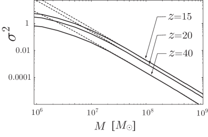
Figure 1: The redshift evolution of the mass dispersion of the density perturbation generated by the magnetic fields with $B_{0}=0.7$ nGauss and $n=1$. The solid lines are the mass dispersion at $z=15$, $z=20$ and $z=40$ (from top to bottom). The dotted lines are the mass dispersion without considering the effect of the magnetic Jeans oscillations.

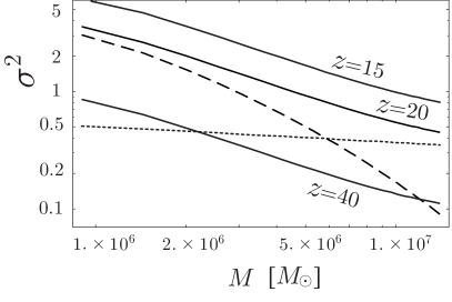
Figure 2: The redshift evolution of the mass dispersion for the model with $B_{0}=0.7$ nGauss and $n=1$. The solid lines represent the total mass dispersion at $z=15$, $z=20$ and $z=40$ (from top to bottom). The dotted and dashed lines are the contributions from $P_{\rm mP}$ and $P_{\rm mM}$, respectively, at $z=20$.

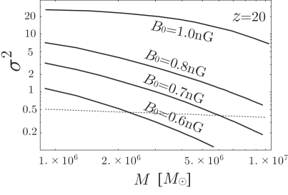
Figure 3: Mass dispersions of models with different strengths of the magnetic fields. The solid lines show the contributions from the magnetic fields of $1.0$ nGauss, $0.8$ nGauss, $0.7$ nGauss and $0.6$ nGauss (from top to bottom) at $z=20$.

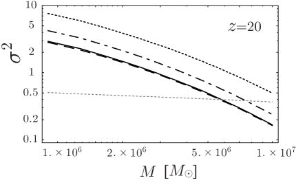
Figure 4: Mass dispersions of models with different spectral indices for the power spectra of the magnetic fields at $z=20$. We fix the strength of the magnetic fields as $0.7$ nGauss. The dotted, dotted-dashed, solid, dashed lines (from top to bottom) are the models with $n=-2$, $-1$, $1$ and $2$, respectively. The thin dotted line is the contribution from the primordial perturbations.

3.2 The ionization photon number

We assume that the Population III stars are formed in collapsed haloes with masses larger than $M_{\rm crit}$ and lower than $M_{\rm vir}$. Here we adopt $M_{\rm crit}=1.0\times 10^{6}~{}h^{-1}M_{\odot}$ and $M_{\rm vir}=M(T_{\rm vir}=10^{4}{\rm K})$ where $M(T_{\rm vir})$ is the virial mass with temperature $T_{\rm vir}$. The virial mass $M(T_{\rm vir})$ evolves as $(1+z)^{-1}$ for given temperature $T_{\rm vir}$. At $z=15$, the virial mass with $T_{\rm vir}=10^{4}$ is $M(T_{\rm vir}=10^{4})=5.2\times 10^{6}M_{\odot}$.

Following the Press-Schechter prescription, we can derive the fraction of the collapse haloes with masses larger than $M$ at time $t$ as

$$F(>M,t)=1-\int^{\delta_{\rm c}}_{0}dx{\sqrt{2}\over\sqrt{\pi}\sigma(M,t)}\exp\left(-{1\over 2}{x^{2}\over\sigma^{2}(M,t)}\right),$$ (21)

where $\sigma^{2}(M,t)$ is obtained by substituting Eq. (20) into Eq. (19).

From $F$, the global star-formation-rate density of the Population III stars can be calculated as

$$\dot{\rho}_{*}(t)=e_{*}\rho_{\rm b}{d\over dt}\left[F(>M_{\rm crit},t)-F(>M_{\rm vir},t)\right],$$ (22)

where $e_{*}$ is the efficiency of conversion of gas into stars and we adopt $e_{*}=0.001$ (Yoshida et al., 2003).

Now we assume that the lifetime of Population III stars is $\Delta t=3\times 10^{6}$ yr. and the production rate of ionizing photons by Population III stars is $N_{\gamma,0}=1.6\times 10^{48}$ photons $s^{-1}M^{-1}_{\odot}$ (Bromm et al., 2001). Accordingly we obtain the total production rate of ionizing photons as

$$\dot{n}_{\gamma}(t) = \int^{t}_{t_{\rm i}}dt^{\prime}N_{\gamma,0}\theta(\Delta t-(t-t^{\prime}))\dot{\rho}_{*}(t^{\prime})$$ (23)

$$= N_{\gamma,0}\left[\rho_{*}(t)-\rho_{*}(t-\Delta t)\right],$$

where $\theta(t)$ is a step function which is $\theta(t)=1$ for $t\geq 0$ and $\theta(t)=0$ for $t<0$.

The cumulative number of photons per H atom is a good indicator of the ionization degree of IGM. It is known that about 20 cumulative photons per H atom are requited in order to achieve a volume weighted ionization of 99 percent (Haiman et al., 2001; Sokasian et al., 2003, 2004). From Eq. (23), the cumulative photons per H atom at time $t$ is represented as

$${n^{\rm cumul}_{\gamma}\over n_{\rm H}}(t) = {\mu m_{\rm p}\over\rho_{\rm b}}\int^{t}_{0}dt^{\prime}\dot{n}_{\gamma}(t^{\prime})$$ (24)

$$= N_{\gamma,0}{\mu m_{\rm p}\over\rho_{\rm b}}\int^{t}_{0}dt^{\prime}\left[\rho_{*}(t^{\prime})-\rho_{*}(t^{\prime}-\Delta t)\right],$$

where $n_{\rm H}$ is the Hydrogen number density, $\mu$ is the mean molecular weight, and $m_{\rm p}$ is the proton mass.

We show cumulative photons from the Population III stars per H atom as a function of redshift. In Fig. 5, the cumulative photons are plotted for different values of the magnetic strength $B_{0}$. Here we fix $n=1$. It is found that more photons are produced as the magnetic field strength becomes stronger since the amplitude of the density perturbations depends on the strenth. We can conclude that the universe is reionized early enough to be consistent with WMAP data if $B_{0}$ is larger than $0.7$ nGauss. Remember that 20 cumulative photons are needed to achieve a 99 percent volume weighted ionization.

If the magnetic field strength is larger than $1$nGauss, however, it is shown that the cumulative photons become smaller as we increase the strength since the magnetic Jeans scale shifts to the larger scale which makes Population III stars difficult to be formed. We found that the magnetic fields larger than $1.5$ nGauss cannot generate large enough number of cumulative photons to induce early reionization.

Fig. 6 shows the dependence of the cumulative photons on $n$. It is found that there is little dependence if $n>-1.5$. Therefore the requirement $B_{0}\ga 0.7$ nGauss for early reionization is robust regardless of the power law index of the magnetic fields.

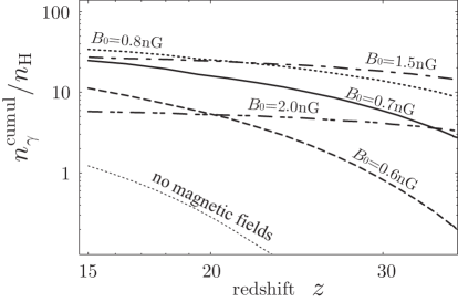
Figure 5: The cumulative photons from the Population III stars per H atom for the models with the magnetic fields. The spectral index of the magnetic fields is fixed as $n=1$. The strengths of the magnetic fields are $2.0$, $1.5$, $0.8$, $0.7$ and $0.6$ nGauss for the dashed–dotted-dotted, dashed–dotted, dotted, solid and dashed lines, respectively. The thin dotted line is the case with no magnetic fields.

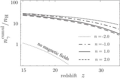
Figure 6: The cumulative photons from the Population III stars per H atom for the models with the fixed strength of magnetic fields $0.7$ nGauss and various spectral indices. The dotted, dotted-dashed, solid, dashed lines (from top to bottom) are the models with $n=-2$, $-1$, $1$ and $2$, respectively. It is shown that dependence on $n$ of the cumulative photons is very weak. The thin dotted line is for the case of no magnetic fields.

4 conclusion

In this paper we investigate the role of the additional density perturbations generated by the primordial magnetic fields on the reionization process in the early universe. These additional density perturbations may trigger the early structure and star formation. Employing a simple analytic recipe, we estimate the number of ionizing photons emitted from the Population III stars. We found that the reionization process almost completes by $z\sim 15$ if the strength of primordial magnetic fields is larger than $0.7$ nGauss and less than $1.5$ nGauss. Note that we adopt the Gaussian window function to calculate the mass dispersion (see Eq. (19)). Different choice of the window function alters the mass dispersion at the magnetic Jeans scale. Accordingly the magnetic field strength to be required for the early enough reionization is also changed. If we employ the sharp-$k$ window function, for example, the strength should be between $0.5$ and $0.7$ nGauss.

Such magnetic fields are not yet ruled out from current observations, i.e., BBN, CMB temperature anisotropies and polarization, and Faraday rotation of polarized lights from radio sources. Although the formation process of such primordial magnetic fields is still uncertain, magnetic fields may be naturally generated during the cosmological phase transition (Banerjee & Jedamzik, 2004).

The extra-power of the matter power spectrum will be directly probed by future observations such as the fluctuations of the Hydrogen 21cm line (Loeb & Zaldarriaga, 2004) and the substructure of lensing haloes (Dalal & Kochanek, 2002). Moreover, the thermal diffusion process of primordial magnetic fields may cause ionization of IGM even before Population III stars. A measurement of fluctuations of the 21cm line will be a powerful tool to investigate such pre-reionization (Tashiro & Sugiyama, in preparation).

References

- Avelino & Liddle (2004) Avelino P. P., Liddle A. R., 2004, MNRAS, 348, 105
- Banerjee & Jedamzik (2004) Banerjee R., Jedamzik K., 2004, Phys. Rev. D, 70, 123003
- Becker et al. (2001) Becker R. H., Fan X., White R. L., Strauss M. A., Narayanan V. K. et al., 2001, Astron. J., 122, 2850
- Brandenburg & Subramanian (2005) Brandenburg A., Subramanian K., 2005, Phys. Rep., 417, 1
- Bromm et al. (2001) Bromm V., Kudritzki R. P., Loeb A., 2001, ApJ, 552, 464
- Cen (2003) Cen R., 2003, ApJ, 591, 12
- Chen et al. (2003) Chen X., Cooray A., Yoshida N., Sugiyama N., 2003, MNRAS, 346, L31
- Cheng et al. (1996) Cheng B., Olinto A. V., Schramm D. N., Truran J. W., 1996, Phys. Rev. D, 54, 4714
- Ciardi et al. (2003) Ciardi B., Ferrara A., White S. D. M., 2003, MNRAS, 344, L7
- Dalal & Kochanek (2002) Dalal N., Kochanek C. S., 2002, ApJ, 572, 25
- Fan et al. (2002) Fan X., Narayanan V. K., Strauss M. A., White R. L., Becker R. H., et al., 2002, Astron. J., 123, 1247
- Fukugita & Kawasaki (2003) Fukugita M., Kawasaki M., 2003, MNRAS, 343, L25
- Giovannini (2004) Giovannini M., 2004, International Journal of Modern Physics D, 13, 391
- Gopal & Sethi (2003) Gopal R., Sethi S. K., 2003, Journal of Astrophysics and Astronomy, 24, 51
- Haiman et al. (2001) Haiman Z., Abel T., Madau P., 2001, ApJ, 551, 599
- Haiman & Holder (2003) Haiman Z., Holder G. P., 2003, ApJ, 595, 1
- Jedamzik et al. (1998) Jedamzik K., Katalinić V., Olinto A. V., 1998, Phys. Rev. D, 57, 3264
- Jedamzik et al. (2000) Jedamzik K., Katalinić V., Olinto A. V., 2000, Physical Review Letters, 85, 700
- Kernan et al. (1996) Kernan P. J., Starkman G. D., Vachaspati T., 1996, Phys. Rev. D, 54, 7207
- Kim et al. (1996) Kim E.-J., Olinto A. V., Rosner R., 1996, ApJ, 468, 28
- Kim et al. (1990) Kim K.-T., Kronberg P. P., Dewdney P. E., Landecker T. L., 1990, ApJ, 355, 29
- Kim et al. (1991) Kim K.-T., Kronberg P. P., Tribble P. C., 1991, ApJ, 379, 80
- Kogut et al. (2003) Kogut A., Spergel D. N., Barnes C., Bennett C. L., Halpern M., et al., 2003, ApJS, 148, 161
- Kronberg (1994) Kronberg P. P., 1994, Reports of Progress in Physics, 57, 325
- Kronberg et al. (1992) Kronberg P. P., Perry J. J., Zukowski E. L. H., 1992, ApJ, 387, 528
- Lewis (2004) Lewis A., 2004, Phys. Rev. D, 70, 043011
- Loeb & Barkana (2001) Loeb A., Barkana R., 2001, ARA&A, 39, 19
- Loeb & Zaldarriaga (2004) Loeb A., Zaldarriaga M., 2004, Physical Review Letters, 92, 211301
- Mack et al. (2002) Mack A., Kahniashvili T., Kosowsky A., 2002, Phys. Rev. D, 65, 123004
- Seljak et al. (2005) Seljak U., Makarov A., McDonald P., Anderson S. F., Bahcall N. A. et al., 2005, Phys. Rev. D, 71, 103515
- Seljak & Zaldarriaga (1996) Seljak U., Zaldarriaga M., 1996, ApJ, 469, 437
- Sethi & Subramanian (2005) Sethi S. K., Subramanian K., 2005, MNRAS, 356, 778
- Sokasian et al. (2003) Sokasian A., Abel T., Hernquist L., Springel V., 2003, MNRAS, 344, 607
- Sokasian et al. (2004) Sokasian A., Yoshida N., Abel T., Hernquist L., Springel V., 2004, MNRAS, 350, 47
- Somerville & Livio (2003) Somerville R. S., Livio M., 2003, ApJ, 593, 611
- Spergel et al. (2003) Spergel D. N., Verde L., Peiris H. V., Komatsu E., Nolta M. R. et al., 2003, ApJS, 148, 175
- Subramanian & Barrow (1998) Subramanian K., Barrow J. D., 1998, Phys. Rev. D, 58, 083502
- Sugiyama et al. (2004) Sugiyama N., Zaroubi S., Silk J., 2004, MNRAS, 354, 543
- Tashiro & Sugiyama (in preparation) Tashiro H., Sugiyama N., in preparation
- Tashiro et al. (2006) Tashiro H., Sugiyama N., Banerjee R., 2006, Phys. Rev. D, 73, 023002
- Wasserman (1978) Wasserman I., 1978, ApJ, 224, 337
- Widrow (2002) Widrow L. M., 2002, Reviews of Modern Physics, 74, 775
- Yamazaki et al. (2005) Yamazaki D. G., Ichiki K., Kajino T., 2005, ApJl, 625, L1
- Yoshida et al. (2003) Yoshida N., Abel T., Hernquist L., Sugiyama N., 2003, ApJ, 592, 645
- Zeldovich et al. (1983) Zeldovich I. B., Ruzmaikin A. A., Sokolov D. D., 1983, Magnetic fields in astrophysics, The Fluid mechanics of astrophysics and geophysics;vol. 3, Gordon and Breach, New York