A MMT/HECTOSPEC REDSHIFT SURVEY OF 24 MICRON SOURCES IN THE SPITZER FIRST LOOK SURVEY

Abstract

We present a spectroscopic survey using the MMT/Hectospec fiber spectrograph of 24 µm sources selected with the Spitzer Space Telescope in the Spitzer First Look Survey. We report 1296 new redshifts for 24 µm sources, including 599 with $f_{\nu}(24\micron)\geq 1$ mJy. Combined with 291 additional redshifts for sources from the Sloan Digital Sky Survey (SDSS), our observing program was highly efficient and is $\sim$90% complete for $\hbox{$i$}\leq 21$ mag and $f_{\nu}(24\micron)\geq 1$ mJy, and is 35% complete for $\hbox{$i$}\leq 20.5$ mag and 0.3 mJy $\leq f_{\nu}(24\micron)<$1.0 mJy. Our Hectospec survey includes 1078 and 168 objects spectroscopically classified as galaxies and QSOs, respectively. Combining the Hectospec and SDSS samples, we find 24 µm–selected galaxies to $z_{\mathrm{gal}}\leq 0.98$ and QSOs to $z_{\mathrm{QSO}}\leq 3.6$, with mean redshifts of $\langle z_{\mathrm{gal}}\rangle$=0.27 and $\langle z_{\mathrm{QSO}}\rangle$=1.1. As part of this publication, we include the redshift catalogs and the reduced spectra; these are also available through the NASA/IPAC Infrared Science Archive.

1 Introduction

Observations with the Infrared (IR) Astronomical Satellite (IRAS) discovered that much of the bolometric emission associated with star–formation and active–galactic nuclei occurs in the thermal infrared. The analysis of IRAS sources indicated that most ($\simeq$70%) of the light emitted from local, normal galaxies comes at UV and optical wavelengths (e.g. Soifer & Neugebauer, 1991). However, measurements of the IR background found that the total far–IR emission ($\lambda=8-1000$ µm) of galaxies is comparable to that measured at UV and optical wavelengths (e.g., Hauser et al., 1998). Therefore, over the history of the Universe, roughly half of the photons from star formation or black–hole accretion processes are emitted at IR wavelengths (Elbaz et al., 2002; Dole et al., 2006). Subsequent studies of IR number counts from the Infrared Space Observatory (ISO; Elbaz et al. 1999) and more recently from the Spitzer Space Telescope (Marleau et al., 2004; Papovich et al., 2004) showed that IR–luminous galaxies have evolved rapidly, implying that they are a much more common phenomenon at high redshifts.

Studying the increase in the IR–active phases of galaxies requires measuring the properties of these objects as a function of redshift. Observations at 24 µm from the multiband imaging photometer for Spitzer (MIPS, Rieke et al., 2004) are particularly well suited for such studies. Soifer, Neugebauer, & Houck (1987) concluded that starburst galaxies radiate as much as $\sim$40% of their luminosity in the mid–IR (8–40 µm). The mid–IR emission from starforming galaxies correlates almost linearly with total IR luminosity over a range of galaxy type (e.g., Spinoglio et al., 1995; Roussel et al., 2001; Papovich & Bell, 2002; Calzetti et al., 2005). The angular resolution of Spitzer at 24 µm is roughly a factor of 3 and 7 better than that at 70 and 160 µm, respectively, allowing unambiguous source identification and probing the IR emission from many more sources than at the longer wavelengths. Already, early studies of Spitzer 24 µm sources with photometric redshifts over relatively small fields ($\lesssim 0.5$ sq. deg) indicate that the bright end of the IR luminosity function evolves strongly from $z\sim 0$ to 1 (Le Floc’h et al., 2005; Pérez-González et al., 2005).

To improve our understanding of the nature and evolution of IR-luminous phases of galaxies, we first need to construct large samples of objects with spectroscopic redshifts. In this paper, we publish the results of our survey with the MMT/Hectospec multi-fiber spectrograph in the Spitzer First Look Survey (FLS). We report new redshifts for 1296 objects selected in the $i$–band and at 24 µm over 3.3 deg². Here we publish the catalogs and reduced, flux–calibrated spectra. We are currently using these spectroscopic data in conjunction with surveys in other fields to study the evolution of the IR–luminous galaxy population.

We organize this paper as follows. In § 2, we discuss the Spitzer FLS dataset, our 24 µm catalog, and our spectroscopic target selection. In § 3 we describe the spectroscopic observations and data reduction. In § 4 we discuss the spectroscopic completeness of the catalog. In § 5 we present the Hectospec spectra and redshift catalog. In § 6 we summarize our results and discuss the redshift distribution of our sample of 24 µm sources. All magnitudes in this paper correspond to the AB system (Oke & Gunn, 1983), where $m_{\mathrm{AB}}=23.9-2.5\log(f_{\nu}/1\;\mu\mathrm{Jy})$.

2 Spitzer First Look Survey

2.1 Overview

The Spitzer FLS was a service to the Spitzer user community, initiated as a Director’s Discretionary Time program. The program goal was to provide data over large areas in time to have an impact on early Spitzer studies and proposals. The FLS includes three components, described at http://ssc.spitzer.caltech.edu/fls. Here, we focus on the extragalactic component, whose field was chosen to have low Galactic background and to be in the Spitzer continuous viewing zone (CVZ) such that it would be observable shortly after the Spitzer in-orbit checkout regardless of launch date.

The Spitzer FLS overlaps with imaging and spectroscopic observations from the Sloan Digital Sky Survey (SDSS; York et al., 2000). We use the SDSS imaging data to identify objects in the Spitzer/MIPS data for spectroscopic follow-up.

2.2 MIPS 24 µm Observations and Data

Spitzer observed the FLS during December 2003 (PID: 26; PI: B. T. Soifer). The MIPS observations consisted of medium–speed scan maps (AORKEYS: 3863808, 3864064, 3864320, 3864576, 3864832, 3865088, 3865344, 3865600, 3865856, 3866112, 3866368, 3866624). These 24 µm data cover roughly a field of 4.4 deg² at a depth of 90 sec (the “Shallow”, or “Main” field). Subsequent deeper observations (450 sec) were taken over a smaller field (0.26 deg²; the “Verification” field), but those data were not available prior to our MMT/Hectospec run. Thus, we use only the shallower–depth data over the larger field of view. See Marleau et al. (2004) for more details of the MIPS 24 µm dataset.

We retrieved the raw Spitzer/MIPS 24 µm data from the Spitzer archive and reduced them using the Data Analysis Tool (DAT) designed by the MIPS Guaranteed Time Observers (GTOs; Gordon et al. 2005). The measured count rates were corrected for dark current, cosmic rays, and flux nonlinearities, and then normalized by flat fields appropriate for each MIPS scan–mirror position. Images were then mosaicked after correcting for geometric distortion with a final plate scale of $1\farcs 247$ pixel^-1.

We constructed a catalog from the reduced and mosaicked 24 µm image using SExtractor (Bertin & Arnouts, 1996); table 1 gives the main parameters. We measured photometry in circular apertures of radius $12\farcs 3$. To convert these to total count rates, we applied an aperture correction of 1.172 based on a curve–of–growth analysis of the 24 µm point spread function (PSF), and we converted these to flux density using the current calibration factor. For our primary and secondary spectroscopic targets, we selected the relatively bright MIPS sources with $f_{\nu}(24\micron)\geq 300$ $\mu$Jy (see § 2.3) and required that sources come from regions of the image with exposure time greater than 80 sec. Aperture–photometry for these bright 24 µm objects is fairly robust. Using aperture photometry from SExtractor, Marleau et al. (2004) demonstrated that the scatter between 24 µm flux densities for objects in the overlap region between the FLS shallow and verification fields is less than $\approx$20%. Our tests on the shallow FLS 24 µm image show that in apertures of radius $12\farcs 3$ the 1$\sigma$ flux uncertainty is $\simeq$120 $\mu$Jy. Therefore, the photometric measurements for objects with $f_{\nu}(24\micron)>1$ mJy have high signal–to–noise ratios (S/N$\gtrsim 8$), although photometric uncertainties on objects with $f_{\nu}(24\micron)\sim 0.3$ mJy are higher (S/N$\sim$2–3). Note that the signal–to–noise ratios are significantly higher in the (smaller) isophotal detection apertures. The flux uncertainty of $\sim$120 $\mu$Jy discussed above is only on the measurement in the larger photometric apertures.

The depth of the MIPS 24 µm data for the FLS is comparable to those of the NOAO deep wide–field survey (NDWFS) in the constellation Boötes (e.g., Houck et al., 2005), for which the 24 µm data is roughly 80% complete for sources above 270 $\mu$Jy (Papovich et al., 2004). Similarly, Marleau et al. (2004) estimate the 80% completeness for the FLS 24 µm data at 230 $\mu$Jy. We expect a similar completeness level in the FLS 24 µm catalog used here. However, both Marleau et al. and Papovich et al. used aperture photometry weighted by the 24 µm PSF, providing more accurate photometry vis–á–vis simple aperture photometry especially for fainter sources (particularly, e.g., at $f_{\nu}(24\micron)\lesssim 300$ $\mu$Jy; see Marleau et al.). Therefore, we expect more scatter in the catalog used here particularly at faint flux densities, reducing the overall catalog completeness (see also § 2.3). For this reason and owing to the higher photometric uncertainties discussed above, the accuracy of the 24 µm flux densities below $\lesssim 0.5$ mJy may be insufficient for some applications.

2.3 Spectroscopic Target Selection

We selected MIPS 24 µm sources from our catalog as spectroscopic targets using the SDSS $i$-band photometry (Stoughton et al., 2002). We matched the MIPS 24 µm sources to SDSS $i$–band objects from Data Release 2 (rerun 40–44, Abazajian et al., 2004) within a radius of 2″ down to $\hbox{$i$}\leq 21$ mag, excluding objects saturated in SDSS. We used the combined–model (cmodel) magnitude for our $i$-band photometry. The SDSS fits seeing–convolved elliptical de Vaucouleurs and exponential models to the deblended images. The cmodel aperture goes one step further by finding the best non-negative linear combination of the two (de Vaucouleurs and exponential) best fit models. The parameter of this mixture is listed as frac_deV in the SDSS data releases. The cmodel flux is taken as this linear combination of the best–fit model fluxes. Tests have shown that this combination tracks the Petrosian magnitudes well but with improved performance for fainter and smaller objects (Abazajian et al., 2004).

The SDSS deblender algorithm does not typically separate sources closer than $\sim$2–4″ (e.g., Pindor et al., 2003). Although the MIPS 24 µm PSF is $6\arcsec$ FWHM, source centroiding is accurate to $<$1″. Therefore, we expect few cases where multiple SDSS sources lie within 2″ of a 24 µm source. In fact, we find that there are only 10 MIPS sources with 2 SDSS associations ($<$0.3% of the matched 24 µm–SDSS sample; no MIPS source has more than 2 associations in SDSS). In these cases, we associate the 24 µm source with both SDSS sources in our catalogs for completeness. In practice, we placed Hectospec fibers on only 2 of these 20 SDSS galaxies, both of which are Galactic stars. Therefore, the few 24 µm sources with multiple object associations in SDSS has a tiny impact on our survey. However, there may still be some cases where the 24 µm–matched SDSS source is not the true association (i.e., the true optical counterpart is fainter than the SDSS detection limit). Alternatively, it may also be that the separation between the SDSS optical counterpart and the 24 µm source is $>$2″, as may be the case for nearby galaxies where the optical centroid is offset from the 24 µm centroid.

To target objects for spectroscopy, we constructed a three–tiered sample:

$$\begin{array}[]{lrcl}\mathrm{Primary~{}\;Sample,}&\;\;f_{\nu}(24\micron)\geq 1.0\mathrm{~{}mJy}&\mathrm{and}&\hbox{$i$}\leq 21\mathrm{~{}mag};\\ \mathrm{Secondary~{}\;Sample,}&\;\;\;0.3\mathrm{~{}mJy}\leq f_{\nu}(24\micron)<1.0\mathrm{~{}mJy}&\mathrm{and}&\hbox{$i$}\leq 20.5\mathrm{~{}mag};\\ \mathrm{Tertiary~{}\;Sample,}&\;\;f_{\nu}(24\micron)<0.3\mathrm{~{}mJy}&\mathrm{and}&\hbox{$i$}\leq 20.5\mathrm{~{}mag}.\end{array}$$ (1)

We exclude all sources with SDSS 3″–aperture fiber magnitudes $\hbox{$r$}\leq 17$ mag; this removes stars brighter than about $\hbox{$r$}<17.3$ but affects very few galaxies. This sample selection identified 1076 sources in the primary sample, 2296 sources in the secondary sample, and 2325 sources in the tertiary sample, corresponding to survey densities of 0.07, 0.14, and 0.15 arcmin^-2 within the FLS shallow field, respectively. This is our parent sample for spectroscopy. Table 2 presents the astrometry and photometry from the SDSS and MIPS 24 µm data for the parent sample. Note that each object in the parent sample is assigned a unique ID number, in column (1) of table 3. These ID numbers are used in subsequent tables to identify the object in the spectroscopic catalogs. The target–flag values (column 9) identifies objects satisfying the primary (Target Flag=2), secondary (Target Flag=4), or tertiary sample (Target Flag=8), as well as calibration stars (Target Flag=1), and other objects ($z$$\sim$0.5 red galaxies, and quasars; Target Flag=0). Note that objects in the tertiary sample and those with Target Flag=0 are primarily used to fill out the fiber configurations, and in general these samples are too sparse to be statistically useful.

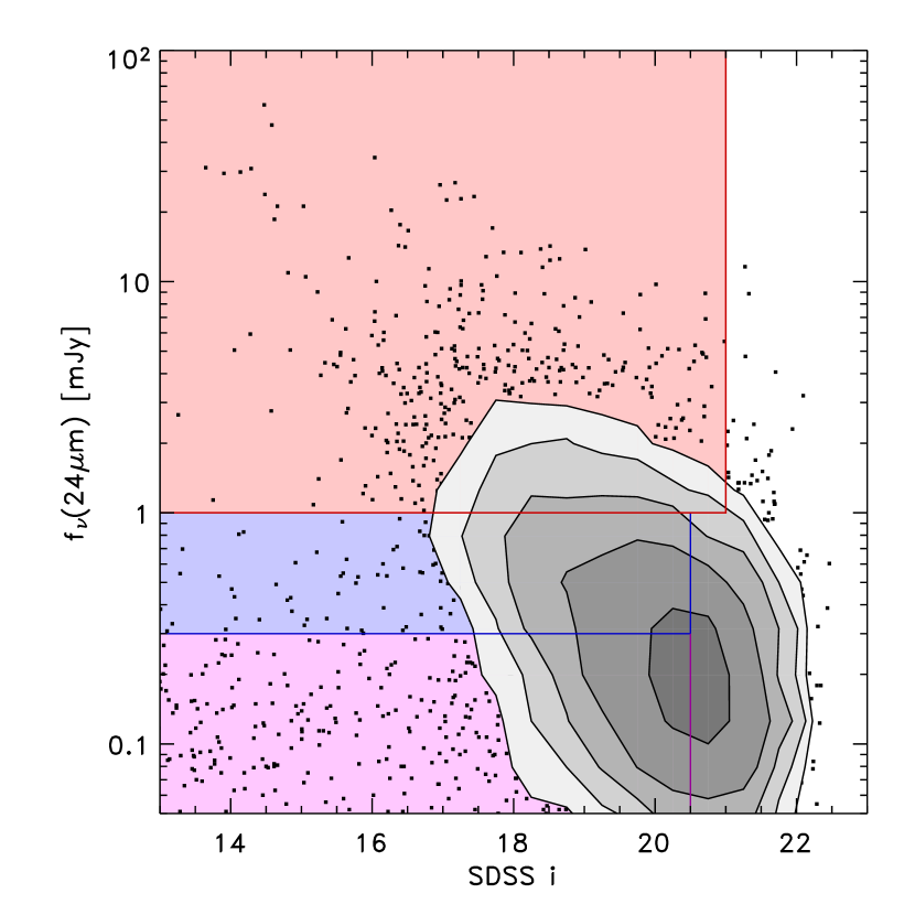
Figure 1: Distribution of 24 µm flux densities of FLS sources as a function of SDSS $i$–band magnitude. We use contours where more than 16 data points fall in bins of $\Delta\hbox{$i$}=0.5$ mag and $\Delta(\log f_{\nu}[24\micron])=0.2$ dex, and we plot individual points otherwise. The first contour corresponds to a source density of 16 objects in these bins, and each contour corresponds to a source density successively higher by a factor of two. Shaded rectangles show target selection for spectroscopy. The red–shaded region shows the primary selection, $f_{\nu}(24\micron)\geq 1$ mJy and $\hbox{$i$}\leq 21$ mag. The blue–shaded region shows the secondary selection, $0.3\leq f_{\nu}(24\micron)/$1 mJy$<1$ and $\hbox{$i$}\leq 20.5$ mag. The magenta–shaded region shows the tertiary selection, $f_{\nu}(24\micron)<0.3$ mJy and $\hbox{$i$}\leq 20.5$ mag. Sources fainter than the $\hbox{$i$}\gtrsim 21.3$ mag will be missed in SDSS.

In figure 1 we illustrate our sample selection on a $i$–band magnitude versus 24 µm flux–density diagram. For this plot, we show all MIPS 24 µm sources with $i$–band counterparts, including sources with $i$$>$21 mag in SDSS. The optical magnitude limit of our primary sample selection includes about 60% of all 24 µm sources with flux densities above 1 mJy. We find that saturated stars (and objects blended with the light from saturated stars) account for 10% of sources with $f_{\nu}(24\micron)\geq 1$ mJy, and a further 5% are galaxies where there exists a large centroiding offset between the optical and 24 µm source or where the galaxy is split into multiple 24 µm sources. The remaining 25% of the $f_{\nu}(24\micron)\geq 1$ mJy population corresponds to objects with optical counterparts fainter than $\hbox{$i$}\gtrsim 21$ mag, likely similar to the IR–luminous galaxies and AGN at higher redshift ($z$$\gtrsim$1) studied by Houck et al. (2005), Yan et al. (2005), and Weedman et al. (2006).

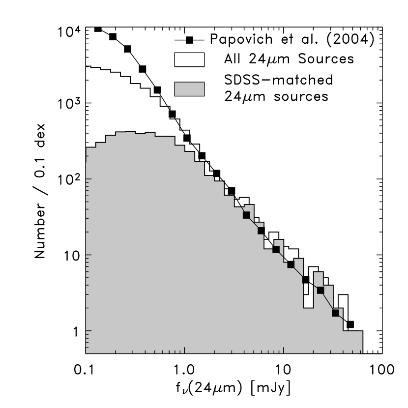
Figure 2: Number distribution of 24 µm sources. The filled histogram shows the SDSS–matched 24 µm sample in flux–density bins of 0.1 dex. The unfilled histogram shows the number distribution of all 24 µm sources in the FLS that fall in the Hectospec fields. For comparison, the solid squares show the expected number distribution for 24 µm sources based on the total number counts from Papovich et al. (2004), normalized to the area of the Hectospec survey (3.3 deg²). The drop in the number of SDSS–matched spectroscopic targets below $\sim$1 mJy occurs because of the optical SDSS magnitude limit (see figure 1). The SDSS–matched sample excludes 40% of the 24 µm sources with $f_{\nu}(24\micron)>1$ mJy. Of these, $\sim$40% are saturated stars and objects too close to saturated stars, nearby galaxies split into multiple 24 µm sources, and objects with a large offset exists between the optical and 24 µm source. The remaining objects (25% of the $f_{\nu}(24\micron)\geq 1$ mJy population) have fainter optical counterparts, $\hbox{$i$}\gtrsim 21$ mag.

The distribution of Spitzer 24 µm sources with fainter flux densities extends to fainter optical magnitudes. Thus, our survey is less complete for 24 µm sources with $f_{\nu}(24\micron)\leq 1$ mJy — we find that the optical magnitude limit of the secondary sample includes $\approx$32% of all sources with 0.3 mJy $\leq f_{\nu}(24\micron)<$ 1 mJy in the Hectospec fields. This incompleteness is illustrated in figure 2, which shows the number counts of SDSS–matched 24 µm sources. Compared with all 24 µm sources in the Hectospec fields, the number distribution of SDSS–matched 24 µmsources is mostly complete for $\gtrsim$1 mJy, then begins to decline as the fraction of 24 µm sources with SDSS–optical counterparts decreases. As a comparison, we show the expected number distribution of 24 µm sources from the total number counts of Papovich et al. (2004).

SDSS provides spectroscopic coverage over the FLS field for objects with $\hbox{$r$}<17.77$ mag. From the SDSS-matched 24 µm catalog, 291 objects have spectroscopic redshifts from SDSS with no warnings on the redshift measurement (ZWARNING=0), split between stars (11), galaxies (223), and QSOs (57). We list the properties of these objects in table 4. ID numbers in column 1 of table 4 correspond to the ID numbers in column 1 of table 3. Because the objects in table 4 have high–quality redshifts and spectra from SDSS, we did not reobserve them with Hectospec.

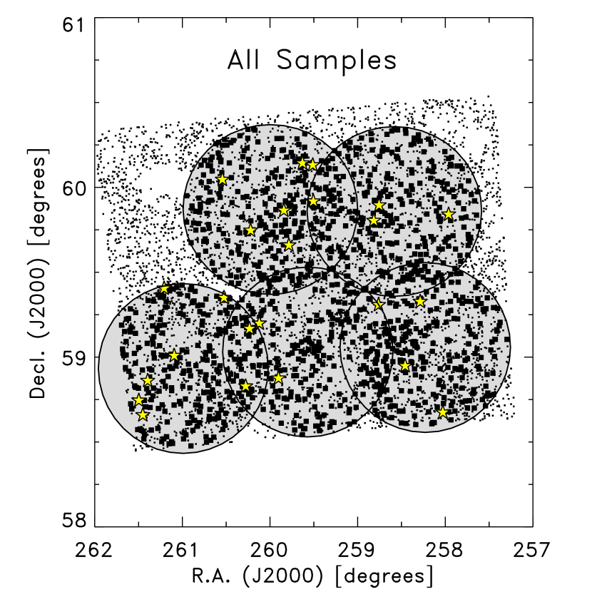
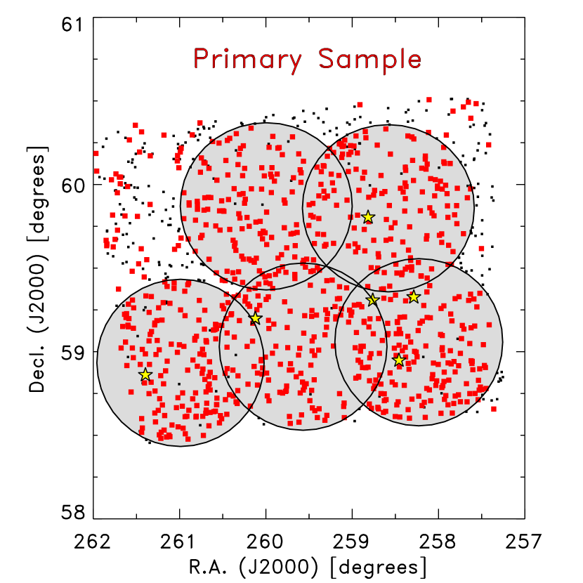
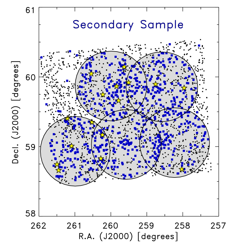
Figure 3: Hectospec field and SDSS–matched 24 µm source locations in the Spitzer FLS. Large shaded circles show the positions of our Hectospec fields, also listed in table 2. The black dots in the top panel show objects from all three MIPS samples. Large, boxes show 24 µm sources with successfully measured extragalactic redshifts from Hectospec only, yellow stars show sources spectroscopically classified as Galactic stars. The bottom panels show only those objects in the primary (1076 objects) and secondary samples (2296 objects), as labeled. In the bottom panels, the large, solid boxes show the 794 primary and 693 secondary sources with redshifts from either Hectospec or SDSS.

3 Observations and Data Reduction

3.1 Observational Layout

Hectospec is a 300–fiber spectrograph covering a 1 degree–diameter field–of–view at the f/5 focus of the 6.5 m MMT (Fabricant et al., 2005). It began routine observing in 2004 April. Each fiber aperture is $1\farcs 5$ diameter, and the resulting spectra cover a wavelength range of $\lambda=3500-9000$ Å with 6 Å FWHM resolution ($R\sim 1000$).

Figure 3 shows the Spitzer FLS layout including the locations of the Hectospec fields, the 24 µm parent sample, and the 24 µm sources with successfully measured redshifts. Each pointing provides some overlap with other pointings on the sky. The total area surveyed by the five Hectospec pointings is 3.3 deg², correcting for the overlap between the fields.

We generated FLS fiber configurations for five different fields, targeting sources from the parent sample defined in § 2.3. We named the configuration fields 131 to 135. We required that Hectospec place fibers on 4–7 spectrophotometric F–type stars selected from SDSS, and we placed $\sim$30 fibers on blank–sky locations to measure the sky brightness. The remaining fibers (typically $>$250) were placed on sources from the parent sample, giving the highest priority to objects in the primary sample, and lowest priority to objects in the tertiary sample. We executed our observations during 2004 July using an exposure time of 45 minutes split into 3$\times$15 minute exposures. Seeing was typically sub-arcsecond. Table 2 summarizes the Hectospec field centers and log for the observations, including the airmass at the time of the observation. In total, we targeted 1291 sources for spectroscopy (605 primary targets, 632 secondary targets, 23 tertiary targets, and 31 filler targets); not including sky or unused fibers, nor calibration stars.

3.2 Data Reduction

We reduced the Hectospec data using HSRED, an IDL package developed by one of us (R. Cool) for the reduction of data from the Hectospec and Hectochelle spectrographs (Fabricant et al., 2005; Szentgyorgyi et al., 1998). HSRED is based heavily on the reduction routines developed for SDSS. Initially, cosmic rays are identified and removed from the two–dimensional images using the IDL version of L. A. Cosmic (van Dokkum, 2001) developed by J. Bloom. Dome flat observations are used to identify the 300 fiber traces on the two–dimensional images. These provide a high–frequency flat field and fringing correction for the object spectra. On nights when twilight sky spectra were obtained, these images were used to derive a low–order correction to the flat field vector for each fiber. We refine the wavelength solution for each observation, originally determined from HeNeAr comparison spectra, using the locations of bright sky lines in each object spectrum. We further use the strengths of several sky features to determine a small amplitude correction for each fiber to remove relative transmission differences between fibers, which are not fully removed by the flat field. The local sky spectrum for each observation is determined using the $\sim$30 dedicated sky fibers, and is then subtracted from each object spectrum.

We flux–calibrate the spectra using simultaneous observations of the F–stars on each Hectospec configuration. The spectral class of each F–star is determined by a comparison against a grid of Kurucz (1993) atmospheric models. The ratio between the observed spectral shape of the F–star and the best fit model provides the shape of the sensitivity function of each fiber. SDSS photometric observations of the standard stars are used to normalize the absolute flux scale. After each exposure is extracted, corrected for helio–centric motion ($\approx$6 km s^-1, given the placement of the FLS in the Spitzer CVZ), and flux calibrated, we de–redden each spectrum according to the Galactic dust maps of Schlegel, Finkbeiner, & Davis (1998) using the O’Donnell (1994) extinction curve. Lastly, we coadd multiple exposures of a field to obtain the final, flux–calibrated spectra.

3.3 Problems with the Atmospheric Dispersion Corrector

Hectospec uses a counter–rotating atmospheric dispersion corrector (ADC) to counteract the atmosphere–induced wavelength–dependent aberration. Unfortunately, during the first few months of Hectospec operation (prior to 2004 October) the ADC was erroneously rotating in the wrong direction. As a result, our spectroscopic data suffer from double the usual wavelength aberration. As guiding is in the visual, light in the blue and red tend to miss the $1\farcs 5$–diameter fiber aperture, in an amount that depends on the surface brightness profile of the object. Point sources suffer more than extended ones.

As discussed in § 3.2, we attempted to flux–calibrate the spectra by matching the spectrophotometric F–type stars for each configuration to a grid of model atmospheres. Because of the atmospheric dispersion, the flux–calibration correction in the blue can be large, and for extended sources, it is typically overcorrected. Even point sources need not have the same calibration due to slight differences in the centroiding of the target within the fiber. Figure 4 shows examples of several flux–calibrated spectra from our data from three different configurations, taken over the range of airmass 1.16–1.35 (see table 2). There is no way to correct for the problem with the ADC, so we do not recommend these data for applications requiring accurately flux-calibrated spectra over long wavelength baselines. However, the flux calibration in the mid-optical, e.g., 5000–7000 Å, should be less affected by the ADC problem and may be useful. Line indices in this wavelength range should be robust, as should flux ratios of lines of comparable wavelength (e.g., [O III$\lambda 5007$]/H$\beta$, H$\alpha$/[N II$\lambda 6585$]). Moreover, the ADC problems do not strongly effect the primary focus of measuring redshifts from the spectra.

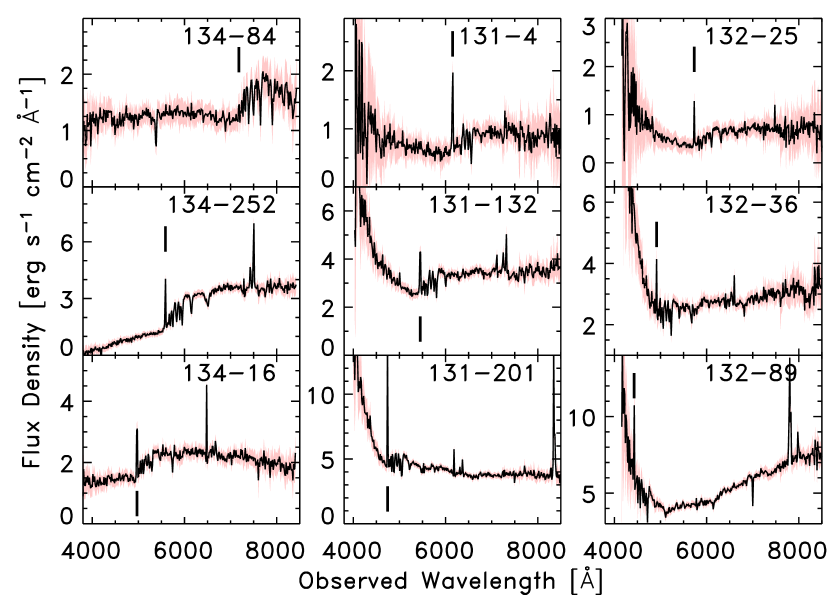
Figure 4: Example spectra from the Hectospec data, illustrating the problem with the atmospheric dispersion corrector. Each panel shows the flux–calibrated spectrum (heavy, black line; resampled to $R\sim 400$ and interpolated over pixels with bad mask values) for a source denoted by its Hectospec field and fiber number. The red, shaded region denotes the 1$\sigma$ uncertainty. The heavy vertical lines denotes the observed wavelength of the [O II] $\lambda$3727 line. The panels are ordered from left to right with increasing airmass at the time the field was observed (see table 2). The increase in flux density at the blue end of the spectrum illustrates the ADC–induced problem with the flux calibration.

3.4 Redshift Measurements

We measured redshifts from the MMT/Hectospec spectra using first an automated pipeline analysis, converted from the SDSS pipeline. We subsequently inspected each spectrum to check the automated measurement. The observing program was highly efficient: of the 1291 science targets for spectroscopy, we measured redshifts successfully for 1270 (a 98% success rate; including both those classified from the automated pipeline and those visually identified).

For our automated measurements, we used a version of the SDSS pipeline specBS (D. Schlegel et al. 2006; http://spectro.astro.princeton.edu) adapted for MMT/Hectospec for the AGN and Galaxy Evolution Survey (AGES) of the NDWFS in the constellation Boötes (Kochanek et al., 2006) and included in the HSRED package (see § 3.2). SpecBS uses $\chi^{2}$ minimization to compare each spectrum to various model spaces, each a linear combination of eigentemplates at different redshifts. The minimum $\chi^{2}$ yields the object’s spectral classification (star, galaxy, QSO, and any sub-classification) as well as the redshift. The classifications are included in table 5. The pipeline also provides a warning flag for the redshift (see § 5).

We then visually inspected the spectra to verify the accuracy of the pipeline–derived redshifts. The automated classification scheme had a high success rate: of the 1291 scientific objects we targeted with fibers, we found that the automated classification algorithm returned faulty or dubious redshifts in only 74 cases (5%). Most of these cases occur in observations at high airmass, where the spectra typically have excessive blue–light flux (see § 3.3). Roughly 50% (36/74) of objects with erroneous redshifts are from field 132 (airmass 1.35). The remaining erroneous redshifts are split fairly evenly between the three configurations taken at moderate airmass (131, 133, and 135). We found only five erroneous redshifts in field 134, with airmass 1.16.

For the majority of spectra with erroneous redshifts (53/74), we identified an alternative redshift by visual inspection. We then remeasured a redshift by fitting a Gaussian to the centroid of strong features in the spectra (normally [O II] or [H$\alpha$], depending on the redshift coverage, and in some cases the Ca H+K doublet) and corrected these to the heliocentric frame. We inserted these remeasured redshifts and uncertainties into the MMT/Hectospec catalog, and set ZVISUALFIXFLAG=1 for these. For these objects, we visually identified the spectroscopic classification as either “Galaxy”, “QSO”, or “STAR”. Note that like SDSS, “QSO” refers to broad–line QSOs; objects identified as a “Galaxy” include also sources that may have putative narrow–line AGN based on broad [O III], H$\alpha$, or line ratios. We also updated the spectroscopic subclassification to “manual” for objects where we remeasured the redshift.

Table 5 lists Hectospec spectroscopic results, including the automated redshifts, redshift uncertainty (columns 10–11), and spectroscopic classification and any subclassification (columns 8 and 9). These entries include objects where we manually measured the redshift, and modified the spectroscopic classification. Objects with visual–flag values of 1 (column 14) correspond to those we judged to have secure redshifts. Although we trust all objects with visual–flag values of 1, for completeness we include the redshift warning flag (ZWARNING; column 12), and reduced $\chi^{2}$ of the redshift fit (column 13) from the automated measurement. We consider objects with visual–flag values of 0 to have untrustworthy redshifts, although we have left the pipeline–derived redshift in the catalog for completeness. Column 4 gives the field number from table 2 of the observation, column 5 gives the Hectospec number of the fiber used to target the object, and column 6 gives the reduction number. The ID numbers in table 5 column 1 correspond to the ID numbers in column 1 of table 3. Most of the objects with visual–flag values of 1 have good automated redshift measurements (with ZWARNING=0; column 12), but 63 of these objects have ZWARNING$>$0. Many of the ZWARNING $>$0 objects have high signal–to–noise spectra, although some (31/63) are ones for which we identified an alternative redshift. Objects with fix–flag values of 1 (ZVISUALFIXFLAG; column 15) correspond to objects for which we visually remeasured an alternative redshift as described above.

As part of the electronic edition of this publication, we present the full photometry and redshift catalog in three separate files. The pertinent information in these three files is given in tables 3–5. The photometry file contains astrometry and photometry from SDSS and MIPS for objects in a parent sample that includes all MIPS sources in the FLS with SDSS matches at $\hbox{$i$}<21$ mag, 37 calibration stars, and 31 other targets that we observed on these configurations as filler targets (see below). Two other files contain the spectroscopic results from the MMT and from the SDSS, respectively. These three files are row synchronous; each file contains 7226 objects, including the 5698 objects in the primary, secondary, and tertiary samples. The ID numbers in column 1 of tables 3–5 correspond to the row of the object in each of the three catalog files.

4 Spectroscopic Completeness

As discussed in § 2.3, our targeting criteria select $\approx$60% of all 24 µm sources with $f_{\nu}(24\micron)\geq 1$ mJy, and $\approx$30% of those sources with 0.3 mJy $\leq f_{\nu}(24\micron)<$ 1 mJy. We did not observe MIPS 24 µm sources with optical magnitudes fainter than $\hbox{$i$}>21$ and 20.5 mag for the primary and secondary samples, respectively.

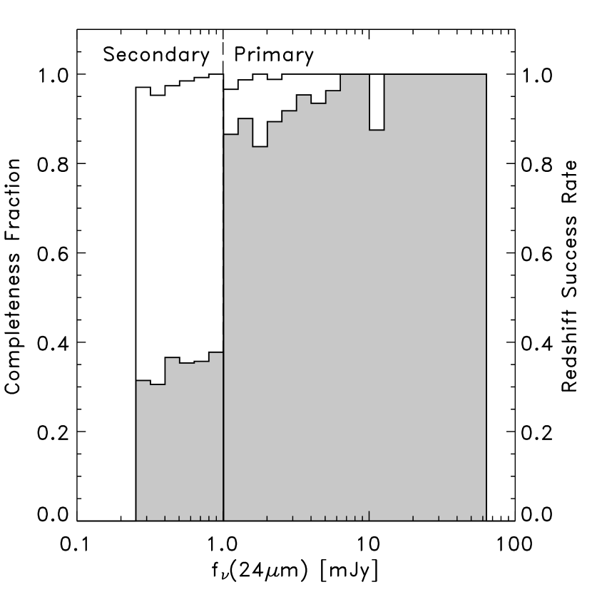
Figure 5: The completeness of the SDSS–matched 24 µm spectroscopic sample as a function of 24 µm flux density. The filled histograms show the completeness fraction of SDSS–matched 24 µm sources with successfully measured redshifts (either from Hectospec or SDSS) to the total number of sources in each sample in the Hectospec region. The unfilled histogram shows the redshift–success rate, defined as the number of sources with successfully measured redshifts to the number of sources observed by Hectospec in each sample. The vertical dashed line delineates the primary and secondary samples (as labeled). The tertiary sample has low completeness ($<$3%), and we do not show it here.

The total spectroscopic success rate is high. We define the redshift–success rate as the ratio of the number of Hectospec targets with measured redshifts to the number of Hectospec targets observed, which we show in figure 5. The redshift success rate for both the primary and secondary samples is 98–99% (599/605 targeted primary sources, and 619/632 targeted secondary sources have successfully measured redshifts).

We compute the overall spectroscopic completeness as the ratio of targets with successfully measured redshifts (including both the MMT/Hectospec and SDSS spectroscopy) to the subsample of targets in the parent sample that fall within our Hectospec fields, i.e., including only those objects that were targets or potential targets for our configurations. Figure 5 shows the spectroscopic completeness as a function of 24 µm flux density. Objects without measured redshifts are counted once for each Hectospec field in which they occur (see figure 3). There are 820 objects in the primary sample falling in the region observed with Hectospec. Of these, 739 have redshifts, with 140 from the SDSS and 599 from our Hectospec program. This is a completeness of 90%. The 10% that were not observed tend to be near the outer edge of the observed region (see fig 3). Hectospec fibers extend nearly radial from the edge of the field of view, and near the edge only one fiber can serve a target, leading to diminishing completeness. Pairs closer than the minimum Hectospec fiber approach of 20″ will also have only one object observed, unless one of the objects was bright enough to be observed by SDSS or unless the pair falls in the overlap region of two MMT pointings. Aside from these minor issues, the primary sample completeness does not have any significant spatial biases.

Of the 1771 objects in the secondary sample falling in the observed region, 662 have redshifts, with 43 from the SDSS and 619 from our Hectospec program (37% completeness). However, we stress that this completeness is highly spatially biased. One can clearly see large-scale structure in the sample that is not being tracked by the subset with spectra. We have not modeled this incompleteness yet, and one should be cautious about using the secondary sample for statistical applications that would be affected by a sampling that depends on the density of targets on the sky.

The tertiary sample is very sparsely covered ($<3$% complete) and should not be used for statistical work.

5 The MMT/Hectospec Spectra

As part of this publication, we make available the fully reduced individual MMT/Hectospec spectra. These data are included as multi-extension FITS (MEF) files as part of the electronic edition of this publication. They are also available through the NASA/IPAC Infrared Science Archive (IRSA; see url in footnote 5). The format of the MEF files for the spectra is similar to those from the SDSS pipeline (http://spectro.astro.princeton.edu). There are 10 Header Data Unit (HDU) extensions in each MEF. Extensions 1–5 contain information for the spectra; these have dimension of $N_{\mathrm{pixel}}\times N_{\mathrm{fiber}}$, where $N_{\mathrm{pixel}}=4608$ is the number of pixels in the spectrum from each fiber and $N_{\mathrm{fiber}}=300$ is the number of fibers. Extension 6 contains targeting information for each fiber. Extensions 7–10 contain information on the flat field and sky spectrum from the data reduction. They are not useful for most applications. The HDUs are:

• HDU 1: Wavelength Solution in Ångstroms in vacuum;

• HDU 2: Flux density of the spectrum in units of $10^{-17}$ erg s^-1 cm^-2 Å^-1;

• HDU 3: Inverse variance ($\sigma^{-2}$) for the flux density;

• HDU 4: Mask of warning flags in each pixel combined between all exposures with logical AND;

• HDU 5: Mask of warning flags in each pixel combined between all exposures with logical OR;

• HDU 6: Structure containing targeting information for each fiber, it contains:

  • OBJTYPE: Type of fiber assignment (target, sky, standard star, or rejected);

  • RA: Right Ascension of fiber (deg; J2000);

  • DEC: Declination of fiber (deg; J2000);

  • FIBERID: Maps aperture to physical fiber on Hectospec;

  • RMAG: SDSS $r$–band magnitude of source;

  • RAPMAG: Estimate of the $r$–band magnitude measured through an aperture with $1\farcs 5$ diameter;

  • ICODE: Integer targeting flags for the observation;

  • RCODE: Not used;

  • BCODE: Not used;

  • MAG: SDSS magnitudes for objects with OBJTYPE equal to standard star;

  • XFOCAL: $x$–coordinate of fiber on Hectospec focal plane;

  • YFOCAL: $y$–coordinate of fiber on Hectospec focal plane;

  • FRAMES: Bookkeeping value from reductions;

  • EXPID: Name of highest–quality exposure;

  • TSOBJID: Not used;

  • TSOBJ_MAG: Bookkeeping values used in spectra flux calibration;

  • EBV_SFD: Galactic extinction, $E(B-V)$, for fiber derived from Schlegel, Finkbeiner, & Davis (1998).

• HDU 7: Structure containing B–Spline parameters for the sky spectrum derived for fibers 1–150;

• HDU 8: Array of dimension $N_{\mathrm{pixel}}\times 150$ containing the auxiliary flat–field correction derived for fibers 1–150 based on strength of sky lines as part of the reduction;

• HDU 9: Same as HDU 6, but for fibers 151–300;

• HDU 10: Same as HDU 8, but for fibers 151–300.

We remind the reader here that the flux calibration suffers from problems arising from the ADC (see § 3.3); caution should be used when using these spectra for applications required accurate flux calibration. The field and fiber value for each object in table 5 correspond to the array for each fiber in MEF for each field.

The data files also contain spectra of 57 objects not part of the MIPS sample. Of these, 26 are calibration stars; the other 31 are from a filler sample of $z\sim 0.5$ red galaxies and quasars, which are far too sparse to be statistically useful.

6 Discussion and Summary

We have obtained 1296 redshifts for Spitzer 24 µm–selected sources in the Spitzer FLS using the Hectospec fiber spectrograph on the MMT. Our observing program was highly efficient ($\simeq$98–99% redshift success rate). It is 90% complete for $f_{\nu}(24\micron)\geq 1$ mJy and $\hbox{$i$}\leq 21$ mag, and is 37% complete for 0.3 mJy $<f_{\nu}(24~{}\micron)<$ 1 mJy and $\hbox{$i$}\leq 20.5$ mag. As part of this publication we provide catalogs for the full parent sample, and the SDSS and MMT redshift catalogs. We also publish our reduced, flux–calibrated spectroscopic Hectospec data.

Our spectroscopic survey of the Spitzer FLS identifies galaxies and QSOs over a large redshift range. Figure 6 shows the redshift distribution for the 24 µm sources from the primary, secondary, and tertiary samples in the FLS, including 1246 sources identified as galaxies and QSOs from our MMT/Hectospec survey, and 280 additional galaxies and QSOs with redshifts from SDSS. Our Hectospec survey of 24 µm sources identifies galaxies to $z\leq 0.98$ and QSOs to $z\leq 3.6$. In figure 7, we show the MMT/Hectospec spectra of the highest redshift objects spectroscopically classified as a galaxy and QSO.

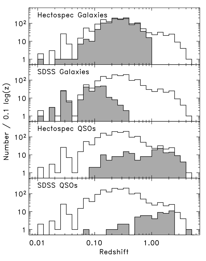
Figure 6: Redshift distribution of 24 µm sources from the combined primary, secondary, and tertiary samples in the Spitzer FLS. In each panel, the shaded histogram shows the redshift distribution (as labeled) of sources spectroscopically classified as “Galaxies”, and “QSOs” from the Hectospec and SDSS data. The solid line shows the redshift distribution of all the MIPS samples from the Hectospec and SDSS samples.

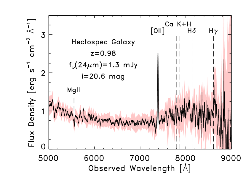
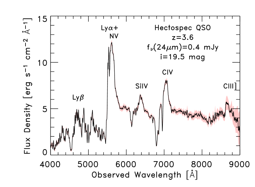
Figure 7: Objects classified as a galaxy and QSO with the highest redshift in the Hectospec data. In each panel, the black, solid line shows the reduced, flux–calibrated Hectospec spectrum (resampled to $R\sim 350$), and the red, shaded region shows the 1$\sigma$ uncertainty. Locations of prominent features are labeled. Redshift, 24 µm flux density, and $i$–band magnitude are inset in each panel.

The redshift distribution for galaxies spans $0.01\lesssim z_{\mathrm{gal}}\lesssim 1$, and the distribution for QSOs extends to higher redshift $0.1\lesssim z_{\mathrm{QSO}}\lesssim 5$. The mean redshifts for galaxies and QSOs (including the Hectospec and SDSS data) are $\langle z_{\mathrm{gal}}\rangle=0.28$ and $\langle z_{\mathrm{QSO}}\rangle=1.1$, with standard deviations of $\sigma_{\mathrm{gal}}=0.17$ and $\sigma_{\mathrm{QSO}}=0.84$. For the primary sample, the mean redshifts for galaxies and QSOs are $\langle z_{\mathrm{gal}}\rangle=0.24$ and $\langle z_{\mathrm{QSO}}\rangle=1.0$, with standard deviations of $\sigma_{\mathrm{gal}}=0.17$ and $\sigma_{\mathrm{QSO}}=0.77$. Similarly, for the secondary sample, the mean redshifts for galaxies and QSOs are $\langle z_{\mathrm{gal}}\rangle=0.31$ and $\langle z_{\mathrm{QSO}}\rangle=1.5$, with standard deviations of $\sigma_{\mathrm{gal}}=0.16$ and $\sigma_{\mathrm{QSO}}=0.94$.

The photometric and redshift catalogs, and reduced spectra are available with the electronic edition of this publication. They are also available through the NASA/IPAC Infrared Science Archive (IRSA; see footnote 5). We are currently pursuing further redshift surveys in Spitzer fields, building the datasets needed to understand the IR–active galaxy population.

Table 1: Main SExtractor Parameters for the 24 µm Catalog

Parameter	Value
DETECT_MINAREA	3.0
DETECT_THRESH	2.5
FILTER	No
DEBLEND_NTHRESH	64
DEBLEND_MINCONT	0.02
CLEAN	Yes
CLEAN_PARAM	1.0
BACK_SIZE	50
BACK_FILTERSIZE	1

Table 2: Target Hectospec Fields

	R.A.	Decl.	$t_{\mathrm{exp}}$	Observation Date
Field	(J2000)	(J2000)	(min)	(UTC)	Airmass
131	17014019.5	+59051029	45	2004 Jun 13	1.23
132	17019059.1	+59052010	45	2004 Jun 13	1.35
133	17012054.9	+59003024	45	2004 Jun 15	1.23
134	17018016.6	+59001048	45	2004 Jun 20	1.16
135	17023057.6	+58055059	45	2004 Jun 23	1.26

Note. — Units of right ascension are hours, minutes, and seconds, and units of declination are degrees, arcminutes, and arcseconds.

Table 3: SDSS–Matched 24 µm Catalog

	R.A.	Decl.	$i$	$u$$-$$g$	$g$$-$$r$	$r$$-$$i$	$i$$-$$z$	$A(r)$	Targ.	$\log f_{\nu}(24\micron)$		R.A. (24µm)	Decl. (24µm)
ID	(J2000)	(J2000)	(mag)	(mag)	(mag)	(mag)	(mag)	(mag)	Flag	(mJy)	SNR24	(J2000)	(J2000)
(1)	(2)	(3)	(4)	(5)	(6)	(7)	(8)	(9)	(10)	(11)	(12)	(13)	(14)
1	17017050.52	+60026048.1	18.01	+1.30	+0.50	+0.15	+0.03	0.066	8	$-$1.33	000.98	17017050.40	+60026047.9
2	17017055.48	+60026039.3	17.59	+1.92	+1.28	+0.50	+0.32	0.066	4	$-$0.15	003.51	17017055.53	+60026039.6
3	17018002.38	+60027020.8	18.60	+1.09	+1.36	+0.51	+0.27	0.067	8	$-$0.74	002.29	17018002.35	+60027020.7
4	17017053.86	+60026020.2	20.36	+2.54	+0.91	+0.40	+0.46	0.065	4	$-$0.40	002.58	17017054.02	+60026021.3
5	17018011.89	+60026049.3	20.19	+1.71	+1.50	+0.39	+0.52	0.066	4	$-$0.39	002.58	17018011.89	+60026049.3
6	17017030.78	+60026037.6	20.84	$-$0.25	+1.59	+0.48	+0.28	0.066	0	$-$0.87	001.46	17017030.95	+60026036.6
7	17018011.34	+60027006.9	20.53	+1.31	+1.53	+0.65	+0.69	0.066	0	$-$0.57	002.71	17018011.33	+60027006.4
8	17018021.07	+60027029.3	20.87	+1.81	+1.67	+0.41	+0.24	0.066	0	$-$1.37	001.08	17018021.08	+60027027.5
9	17018037.32	+60025024.6	19.92	+3.51	+0.98	+0.41	+0.28	0.063	8	$-$1.05	001.25	17018037.49	+60025024.2
10	17017050.77	+60017001.2	16.02	+1.95	+0.90	+0.38	+0.31	0.057	8	$-$1.22	000.94	17017050.86	+60017001.9
11	17018020.37	+60026020.8	20.65	+0.75	+1.02	+0.49	+0.43	0.065	0	$-$0.34	003.10	17018020.41	+60026021.1
12	17018044.49	+60023042.3	18.65	+0.74	+0.95	+0.35	+0.36	0.062	2	+0.62	011.85	17018044.56	+60023041.8
13	17018031.60	+60021000.7	17.29	+1.72	+1.08	+0.52	+0.41	0.059	2	+0.04	005.31	17018031.63	+60021000.8
14	17018033.48	+60026016.9	20.96	+1.42	+1.31	+0.44	+0.24	0.065	0	$-$0.56	002.47	17018033.52	+60026015.6
15	17017041.68	+60025014.3	17.98	+1.18	+0.52	+0.30	+0.12	0.064	8	$-$0.69	002.06	17017041.63	+60025013.0
16	17017034.21	+60023050.7	19.01	+0.27	+0.49	+0.35	+0.27	0.062	2	+0.20	006.64	17017034.23	+60023052.0
17	17017050.54	+60023029.5	19.15	+0.61	+0.66	+0.30	+0.04	0.060	4	$-$0.34	002.83	17017050.67	+60023029.3
18	17018041.06	+60023059.1	19.54	+0.24	+0.22	+0.35	+0.10	0.062	2	+0.02	005.47	17018041.09	+60023058.5
19	17018047.92	+60024009.4	18.73	+1.28	+1.16	+0.34	+0.41	0.062	4	$-$0.10	004.31	17018047.94	+60024009.7
20	17018047.42	+60023030.9	19.55	+0.35	+1.13	+0.38	+0.30	0.062	4	$-$0.25	003.04	17018047.62	+60023030.4

Note. — (1) Row synchronous ID; (2) SDSS right ascension in units of hours, minutes, and seconds; (3) SDSS declination in units of degrees, arcminutes, and arcseconds; (4) SDSS combined–model magnitude (dereddened); (5–8) SDSS combined–model colors (dereddened); (9) Extinction used to deredden magnitudes in (4–8); (10) Hectospec Target Flag (see text); (11) Logarithm of MIPS 24 µm flux density; (12) MIPS 24 µm signal–to–noise ratio, $\equiv f_{\nu}(24\micron)/\delta f_{\nu}(24\micron)$; note that 24 µm flux–density errors do not include correlated pixel noise and are thus underestimated (see text); (13) right ascension of MIPS 24 µm source in units of hours, minutes, and seconds; (14) declinations of MIPS 24 µm source in units of degrees, arcminutes, and arcseconds. Table 3 is published in its entirety in the electronic edition of the Astronomical Journal. A portion is shown here for guidance regarding its form and content.

Table 4: SDSS–Spectoscopic Catalog

	R.A.	Decl.	SDSS information			Targ.
ID	(J2000)	(J2000)	Field	Fiber	Rerun	Code	class	subclass	$z$	$\sigma(z)$	Warn.	$\chi^{2}/\nu$
(1)	(2)	(3)	(4)	(5)	(6)	(7)	(8)	(9)	(10)	(11)	(12)	(13)
10	17017050.76	+60017001.4	354	262	51792	000000064	galaxy	$\cdots$	+0.07923	0.00002	0	1.31
67	17018015.67	+60008022.0	353	612	51703	000000064	galaxy	$\cdots$	+0.15671	0.00001	0	1.38
100	17019044.06	+60002044.6	354	298	51792	000000064	galaxy	$\cdots$	+0.09421	0.00001	0	1.20
107	17018053.16	+60005041.0	354	299	51792	000000064	galaxy	$\cdots$	+0.13285	0.00001	0	1.30
155	17019044.88	+59057006.9	354	290	51792	000000064	galaxy	$\cdots$	+0.06890	0.00001	0	1.34
159	17020007.90	+60001059.7	354	285	51792	000000064	galaxy	$\cdots$	+0.07541	0.00002	0	1.22
255	17020002.11	+59042040.8	353	628	51703	000000004	galaxy	$\cdots$	+0.23937	0.00000	0	1.73
256	17019044.14	+59041001.0	354	292	51792	000000064	galaxy	AGN	+0.12926	0.00001	0	2.03
258	17020009.50	+59040030.1	354	289	51792	000000064	galaxy	$\cdots$	+0.02760	0.00001	0	1.55
324	17020047.14	+59033014.5	366	338	52017	000000096	galaxy	$\cdots$	+0.07041	0.00002	0	1.29
325	17020041.40	+59032044.3	353	636	51703	001048580	QSO	broadline	+1.18430	0.00037	0	1.47
327	17021002.95	+59033012.9	353	634	51703	000000064	galaxy	$\cdots$	+0.07014	0.00001	0	1.49
369	17020002.83	+59022050.0	353	039	51703	000000000	star	F5	$-$0.00053	0.00002	0	1.15
374	17020019.94	+59024016.5	366	335	52017	000000064	galaxy	$\cdots$	+0.15423	0.00001	0	1.42
377	17021004.75	+59024051.4	366	334	52017	034603008	QSO	broadline	+0.78576	0.00034	0	1.41
380	17020056.71	+59019036.8	366	382	52017	000000064	galaxy	$\cdots$	+0.06710	0.00001	0	1.33
381	17021028.70	+59019041.3	353	040	51703	000000064	galaxy	AGN	+0.06544	0.00001	0	1.66
429	17021052.92	+59011055.5	366	385	52017	000000096	galaxy	$\cdots$	+0.06593	0.00001	0	1.54
430	17020045.22	+59016017.7	353	035	51703	000000064	galaxy	$\cdots$	+0.15352	0.00001	0	1.54
436	17021056.93	+59013057.2	366	390	52017	000000064	galaxy	$\cdots$	+0.06535	0.00001	0	1.26
437	17020055.01	+59011016.8	353	030	51703	000000064	galaxy	$\cdots$	+0.06581	0.00001	0	1.37

Note. — (1) Row synchronous ID; (2) SDSS right ascension of spectroscopic target in units of hours, minutes, and seconds; (3) SDSS declination of spectroscopic target in units of degrees, arcminutes, and arcseconds; (4) SDSS field; (5) SDSS fiber number; (6) SDSS reduction run; (7) SDSS primTarget code (decimal); (8) spectroscopic classification; (9) spectroscopic subclassification; (10) redshift; (11) redshift error; (12) redshift warning, $=$0 is safe value; (13) $\chi^{2}$ per degree of freedom for fit. Table 4 is published in its entirety in the electronic edition of the Astronomical Journal. A portion is shown here for guidance regarding its form and content. The electronic version of this catalog includes an entry for each row in table 3, including null rows with no spectroscopic information.

Table 5: Hectospec–Spectoscopic Catalog

	R.A.	Decl.	Hectospec information			Targ.							Vis.	Fix
ID	(J2000)	(J2000)	Field	Fiber	Rerun	Code	class	subclass	$z$	$\sigma(z)$	Warn.	$\chi^{2}/\nu$	Flag	Flag
(1)	(2)	(3)	(4)	(5)	(6)	(7)	(8)	(9)	(10)	(11)	(12)	(13)	(14)	(15)
54	17018024.87	+60018058.5	132	265	300	4	galaxy	$\cdots$	+0.40845	0.00011	0	1.63	1	0
61	17018023.47	+60011004.1	132	251	300	4	QSO	broadline	+1.42971	0.00078	0	1.03	1	0
65	17019023.05	+60013016.4	132	036	300	2	galaxy	$\cdots$	+0.31870	0.00003	0	1.12	1	0
66	17019026.87	+60013003.7	132	038	300	2	galaxy	$\cdots$	+0.16146	0.00001	0	1.66	1	0
68	17018031.25	+60008032.1	132	255	300	4	star	manual	$-$0.00066	0.00011	0	0.91	1	1
72	17019001.99	+60012018.4	132	004	300	4	galaxy	$\cdots$	+0.17466	0.00004	0	1.53	1	0
74	17018041.04	+60015007.2	132	263	300	4	galaxy	manual	+0.21740	0.00011	0	1.31	1	1
76	17018042.88	+60010000.9	132	266	300	4	galaxy	$\cdots$	+0.27900	0.00004	0	1.23	1	0
79	17018045.97	+60017006.5	132	002	300	2	galaxy	$\cdots$	+0.21761	0.00003	0	1.04	1	0
81	17019027.99	+60017017.6	132	039	300	4	galaxy	$\cdots$	+0.24725	0.00006	0	0.88	1	0
82	17018025.34	+60014011.3	132	268	300	4	galaxy	$\cdots$	+0.62651	0.00006	0	0.93	1	0
88	17018028.76	+60011000.3	132	262	300	2	galaxy	$\cdots$	+0.26943	0.00006	0	0.98	1	0
89	17018057.85	+60010058.0	132	261	300	4	galaxy	$\cdots$	+0.24753	0.00006	0	0.91	1	0
91	17019014.34	+60010042.0	132	008	300	2	galaxy	$\cdots$	+0.23165	0.00002	0	1.19	1	0
96	17018040.72	+60007025.6	132	253	300	1	star	F5	$-$0.00110	0.00001	0	3.15	1	0
98	17018043.49	+60002024.8	132	291	300	2	galaxy	$\cdots$	+0.13305	0.00001	0	2.84	1	0
99	17018042.16	+60003016.6	132	258	300	4	galaxy	$\cdots$	+0.12986	0.00002	0	1.05	1	0
104	17018024.77	+60005017.2	132	256	300	2	galaxy	$\cdots$	+0.12923	0.00001	0	5.08	1	0
109	17018057.82	+60001045.8	132	260	300	4	galaxy	$\cdots$	+0.18926	0.00003	0	0.96	1	0
112	17019028.74	+60003045.1	132	006	300	2	galaxy	$\cdots$	+0.20937	0.00003	0	1.02	1	0
113	17019046.96	+60003042.6	132	031	300	2	galaxy	$\cdots$	+0.27874	0.00001	0	1.09	1	0

Note. — (1) Row synchronous ID; (2) Hectospec right ascension of spectroscopic target in units of hours, minutes, and seconds; (3) Hectospec declination of spectroscopic target in units of degrees, arcminutes, and arcseconds; (4) Hectospec field; (5) Hectospec fiber number; (6) Hectospec reduction run; (7) Hectospec Target code (decimal); (8) spectroscopic classification; (9) spectroscopic subclassification; (10) redshift; (11) redshift error; (12) redshift warning, $=$0 is safe value, $>$0 is safe only if Visual flag in (14) is =1; (13) $\chi^{2}$ per degree of freedom for fit. (14) Visual inspection flag, 1 indicates secure redshift, 0 indicates dubious or insecure redshift; (15) Flag indicates automatic redshift discarded and replaced (see text). Table 5 is published in its entirety in the electronic edition of the Astronomical Journal. A portion is shown here for guidance regarding its form and content. The electronic version of this catalog includes an entry for each row in table 3, including null rows with no spectroscopic information.

References

- Abazajian et al. (2004) Abazajian, K., et al. 2004, AJ, 128, 502
- Bertin & Arnouts (1996) Bertin, E., & Arnouts, S. 1996, A&A, 117, 393
- Calzetti et al. (2005) Calzetti, D., et al. 2005, 633, 871
- Dole et al. (2006) Dole, H., et al. 2006, A&A, in press (astro–ph/0603208)
- Elbaz et al. (2002) Elbaz, D., Cesarsky, C. J., Chanial, P., Aussel, H., Franceschini, A., Fadda, D., & Chary, R. R. 2002, A&A, 384, 848
- Elbaz et al. (1999) Elbaz, D., et al. 1999, A&A, 351, L37
- Fabricant et al. (2005) Fabricant, D. et al. 2005, PASP, 117, 1411
- Gordon et al. (2005) Gordon, K., et al. 2005, PASP, 117, 503
- Hauser et al. (1998) Hauser, M. G., et al. 1998, ApJ, 508, 25
- Houck et al. (2005) Houck, J. R., et al. 2005, ApJ, 622, L105
- Kochanek et al. (2006) Kochanek, C. et al. 2006, in preparation
- Kurucz (1993) Kurucz, R. L. 1993, Kurucz CD–ROM, Cambridge, MA: Smithsonian Astrophysical Observatory
- Le Floc’h et al. (2005) Le Floc’h, E., et al. 2005, ApJ, 632, 169
- Marleau et al. (2004) Marleau, F. R., et al. 2004, ApJS, 154, 66
- Morton (1991) Morton, D. C. 1991, ApJS, 77, 119
- O’Donnell (1994) O’Donnell, J. E. 1994, ApJ, 422, 158
- Oke & Gunn (1983) Oke, J. B., & Gunn, J. E. 1983, ApJ, 266, 713
- Papovich & Bell (2002) Papovich, C., & Bell, E. F. 2002, ApJ, 579, L1
- Papovich et al. (2004) Papovich, C., et al. 2004, ApJS, 154, 70
- Pérez-González et al. (2005) Pérez-González, P. G., et al. 2005, ApJ, 630, 82
- Pindor et al. (2003) Pindor, B., Turner, E. L., Lupton, R. H., & Brinkmann, J. 2003, AJ, 125, 2325
- Rieke et al. (2004) Rieke, G. H., et al. 2004, ApJS, 154, 25
- Roussel et al. (2001) Roussel, H., Sauvage, M., Vigroux, L., & Bosma, A. 2001, A&A, 372, 427
- Schlegel, Finkbeiner, & Davis (1998) Schlegel, D. J., Finkbeiner, D. P., & Davis, M. 1998, ApJ, 500, 525
- Schlegel et al. (2006) Schlegel, D., et al. 2006, in preparation
- Soifer, Neugebauer, & Houck (1987) Soifer, B. T., Neugebauer, G., & Houck, J. R. 1987, ARA&A, 25, 187
- Soifer & Neugebauer (1991) Soifer, B. T. & Neugebauer, G. 1991, AJ, 101, 354
- Spinoglio et al. (1995) Spinoglio, L., Malkan, M. A., Rush, B., Carrasco, L., & Recillas–Cruz, E. 1995, ApJ, 453, 616
- Stoughton et al. (2002) Stoughton, C., et al. 2002, AJ, 123, 485
- Szentgyorgyi et al. (1998) Szentgyorgyi, A. H., Cheimets, P., Eng, R., Fabricant, D. G., Geary, J. C., Hartmann, L., Pieri, M. R., & Roll, J. B. 1998, Proc. SPIE, 3355, 242
- van Dokkum (2001) van Dokkum, P. G. 2001, PASP, 113, 1420
- Weedman et al. (2006) Weedman, D. W., Le Floc’h, E., Higdon, S. J. U., Higdon, J. L., & Houck, J. R. 2006, ApJ, 638, 613
- Yan et al. (2005) Yan, L., et al. 2005, ApJ, 628, 604
- York et al. (2000) York, D. G., et al. 2000, AJ, 120, 1579