Reflections on Reflexions: II. Effects of Light Echoes on the luminosity and spectra of Type Ia Supernovae

Abstract

In this paper we present and discuss the effects of scattered light echoes (LE) on the luminosity and spectral appearance of Type Ia Supernovae (SNe). After introducing the basic concepts of LE spectral synthesis, by means of LE models and real observations we investigate the deviations from pure SN spectra, light and colour curves, the signatures that witness the presence of a LE and the possible inferences on the extinction law. The effects on the photometric parameters and spectral features are also discussed. In particular, for the case of circumstellar dust, LEs are found to introduce an apparent relation between the post-maximum decline rate and the absolute luminosity which is most likely going to affect the well known Pskowski-Phillips relation.

1 Introduction

Due to the crucial role played by Type Ia SNe in modern cosmology (see for example the review by Leibundgut 2001), it is essential to understand the systematics which might affect the recent conclusions about the expansion rate of the Universe. The availability of larger telescopes and the renewed interest for these objects as cosmological probes has opened the possibility of studying in great detail their evolution, an investigation which in the past was feasible for the closest events only. In these last few years, in fact, numerous Ia have been followed with an extensive time coverage as late as one year past maximum light, leading to very interesting results (see for example Benetti et al. 2005).

In two cases, namely those of SN 1991T (Schmidt et al., 1994) and SN 1998bu (Cappellaro et al., 2001; Spyromilio et al., 2004), the spectra at advanced phases were clearly dominated by a phenomenon which had nothing to do with the explosion mechanism but rather with the neighboring environment. In both cases this very atypical behaviour could be explained with the contamination by SN light scattered into the line of sight by dust present in the surroundings of the explosion. The presence of such a phenomenon, also known as light echo (hereafter LE), was later confirmed by high spatial resolution HST imaging (Sparks et al. 1999; Garnavich et al. 2001). Other cases have been discovered for core-collapse SNe like SN 1987A (Crotts, Kunkel & McCarthy, 1989), SN 1993J (Sugerman & Crotts, 2002; Liu, Bregman & Seitzer, 2003), SN 1999ev (Maund & Smartt, 2005) and SN 2003gd (Sugerman, 2005; Van Dyk, Li & Filippenko, 2005). In the most recent years, LEs have been searched also in the case of historical SNe (Romaniello et al., 2005; Krause et al., 2005; Rest et al., 2005).

With the purpose of studying this effect and its possible applications to the analysis of the SN environments and their relation with the SN progenitors, we have started a series of papers on this topic. The first of them (Patat 2005; hereafter Paper I) was dedicated to the general characteristics of LEs, with particular attention to the effects of self absorption on LE luminosity, spectral and colour appearance. In this and subsequent papers we will instead present and discuss applications to known and test cases. In principle, LEs can affect all types of SNe. Due to the young stellar population from which they are supposed to be originated, core-collapse SNe are of course favored with respect to thermonuclear explosions. However, both due to their high homogeneity (which makes the analysis much simpler) and their wide use in cosmology, here we will concentrate on Type Ia only. In particular, the present work deals with the effects of LEs on their luminosity and spectra, in order both to help the observers in disentangling intrinsic features from LE contamination and to understand whether LEs can affect the conclusions reached on their nature.

The paper is organized as follows. After giving a short introduction to the basic concepts of LE modeling in Section 2, in Section 3 we describe the spectral library used in our calculations. The results are then presented and discussed in Section 4 for two different dust geometries, while Section 5 is devoted to the implications on the extinction law. In Section 6 we discuss our findings which are briefly summarized in Section 7.

2 Basic concepts

The LE phenomenon has been presented and discussed in a number of publications and we refer to them the interested reader (see for example the recent review by Sugerman 2003 and the references therein). The detailed description of the formation of a LE spectrum has been outlined in Paper I and, therefore, here we will only shortly recap the basic concepts.

In single scattering approximation, the LE spectrum at a given time $t$ can be expressed as

$$S_{LE}(\lambda,t)=\int_{0}^{t}S^{0}(\lambda,t-t^{\prime})f(\lambda,t^{\prime})\;dt^{\prime}$$ (1)

where $S^{0}(\lambda,t)$ is the intrinsic source (SN) spectrum and $f(\lambda,t)$ is a function that describes the physical and geometrical properties of the dust. If we define $\tau_{d}(\lambda)$ as the optical depth to the SN along the line of sight and $S(\lambda,t)$ is the SN spectrum clean of LE contamination, then

$$S^{0}(\lambda,t)=S(\lambda,t)\;e^{\tau_{d}(\lambda)}$$

If we indicate with $C_{ext}(\lambda)$ the dust extinction cross section, $\omega(\lambda)$ the dust albedo and $g(\lambda)$ the forward scattering degree, in all those cases when there is one single cloud with dust on the line of sight (like in the two examples of Fig. 1), the formal solution of equation (1) can be written as follows (see Paper I):

$$S_{LE}(\lambda,t)=G[g(\lambda),t]\;\omega(\lambda)\;C_{ext}(\lambda)\;e^{\tau_{d}(\lambda)}\;{\cal S}(\lambda,t)$$ (2)

where $G[g(\lambda),t]$ is a time- and wavelength-dependent function that includes dust and dust geometry properties and

$${\cal S}(\lambda,t)=\int_{t-t_{c}}^{t}S(\lambda,t-t^{\prime})\;dt^{\prime}$$ (3)

is the time integrated SN spectrum, where $t_{c}$ is the time taken by the generic iso-delay surface to completely cross the dust cloud. The crossing time depends of course on the dust geometry and, if $t_{c}>t$, the lower integration boundary of Equation 3 has to be replaced with 0.

When the SN is only mildly reddened ($\tau_{d}\ll$1), the resulting LE spectrum is therefore proportional to the product between ${\cal S}(\lambda,t)$ and the extinction cross section. When the optical depth is larger ($\tau_{d}>0.3$), single scattering description must be replaced by the more realistic single scattering plus attenuation approximation (hereafter SSA; see Paper I), which holds for $\tau\leq 1$. In this more refined schema, which takes into account the LE self-absorption, equation (2) becomes

$$S_{LE}(\lambda,t)=G[g(\lambda),t]\;\omega(\lambda)\;C_{ext}(\lambda)\;e^{\tau_{d}(\lambda)-\tau_{eff}(\lambda,t)}\;{\cal S}(\lambda,t)$$ (4)

Figure 1: Schematic representation of dust and LE geometry for example cases A (large dust cloud, $t_{c}>$2 yr; left panel) and B (circumstellar dust shell, $t_{c}=$0.015 yr; right panel) for a generic observation time $t$ ($t\geq$2.0 yrs for Case A and $t\geq$0.05 yrs for Case B). The parabolas represent the iso-delay surface corresponding to some preceding epochs.

where $\tau_{eff}(\lambda,t)$ can be regarded as a weighted LE optical depth at a given time $t$. In general, one has that $\tau_{d}\neq\tau_{eff}$, as in the case sketched in Fig. 1 (left panel), where the SN suffers a larger extinction than the LE. In the cases where the SN and the LE are affected roughly by the same extinction, the two effects tend to compensate and the LE spectrum is again proportional to the product between the observed time integrated SN spectrum ${\cal S}$ and the extinction cross section $C_{ext}$. These formal expressions are useful to understand the principles of the problem and will be used later on to explain the apparent peculiarity reported by Schmidt et al. (1994) in the extinction function (see Section 5). Nevertheless, we note that the exact SSA numerical solution is easy to implement in a code and it offers the advantage of properly taking into account the attenuation effect and the wavelength dependency of all involved quantities. While we refer the reader to Paper I for more details, here we will spend some words to discuss one important geometrical effect, which is related to forward scattering and was only marginally mentioned in our previous paper.

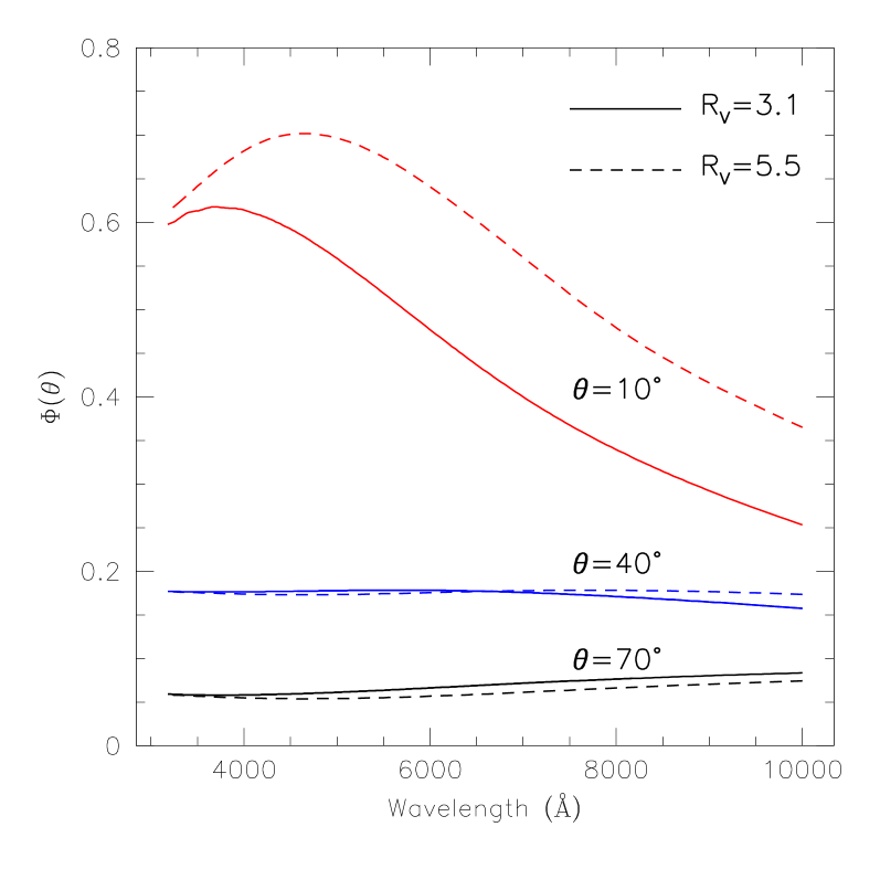
Figure 2: The Henyey-Greenstein scattering phase function $\Phi(\theta)$ computed for three different scattering angles and for $R_{V}$=3.1 and $R_{V}$=5.5. The forward scattering degree function $g$ is from Draine 2003.

In fact, all LE calculations include the so called scattering phase function $\Phi(\theta)$, which describes the probability distribution of photon scattering angle $\theta$ (see for example Chevalier 1986). Usually, this function is parameterized, following Henyey & Greenstein (1941), through the forward scattering degree $g(\lambda)$. To illustrate the behaviour of $\Phi(\theta)$, in Figure 2 we have plotted the results one obtains using the Milky Way dust mixtures modeled by Draine (2003) for $R_{V}$=3.1 (solid lines) and $R_{V}$=5.5 (dashed lines) and for three values of the scattering angle. As one can see, the wavelength dependency is much stronger for lower values of $\theta$, with the scattering being more efficient in the blue than in the red. Therefore, when the dust is located far in front of the SN, which implies a small average scattering angle, the LE spectrum is expected to be bluer than in the case where the same dust, with the same geometry, is placed close to the SN. As a consequence, the same dust cloud can produce the same extinction to the SN (i.e. the same $\tau_{d}$) but different LE colours, according to its position along the line of sight. The simulations show that the $(B-V)$ colour of the LE can change by $\sim$0.15 mag from a configuration where the SN is embedded in the dust cloud to one where the same cloud is placed at more than 200 lyr in front of the SN.

3 Spectral Library

The LE spectral modeling relies on the availability of input SN spectra. For this purpose one needs to build a spectral library with a good phase coverage and time sampling, especially around maximum light. This can be understood inspecting the cumulative functions for the template light curves we discussed in Paper I. These were constructed using the data of SNe 1992A and 1994D, two standard, well studied and low reddening Type Ia (Kirshner et al. 1993; Patat et al. 1996). For $B$ and $V$ passbands, where the LE is expected to be brighter, it turns out that about 90% of the radiation is emitted in 0.2 yr, while the radiation emitted in the first 10 days accounts for about 5% of total. Therefore, the spectral library should include spectra from about a week before maximum to 2-3 months past maximum. Spectra at later epochs are needed only if one is going to extend the calculations to correspondingly late phases for dust geometries with $t>t_{c}$.

Figure 3: Late time spectra of SN 1992A (+328, +406) and SN 1994D (+293). The spectrum at +372 is an average of two spectra of SN 1994D and 1992A at very similar phases. The solid curves in the first three spectra trace the multi-Gaussian fittings. For the +406 spectrum, the solid line is the best fit to the +372 spectrum scaled to match the observations.

We have extended the library used in Paper I, which included only data from SN 1998aq (Branch et al., 2003), adding early and late spectra from SN 1992A (ESO Key-Programme on SNe) and SN 1994D (Patat et al., 1996), so that the data set ranges from $-$11 up to $+$406 days. Irrespective of the original flux calibration, the input spectra have been re-calibrated to make their synthetic $V$ magnitude consistent with the $V$ template light curve. As for the late time spectra, we have used the available data of SNe 1992A and 1994D, which are presented in Figure 3 and reach 406 days past $B$ maximum light. As one can see, the spectra of the two objects remain very similar, also at these late stages. In order to remove the noise in the data, we have used a multi-Gaussian fit to the spectra (solid smooth lines).

Due to the lack of data at later phases, in our calculations we have assumed that after phase +406 there is no evolution and, from that phase on, the SN spectrum is simply scaled according to the exponential decay of the $V$ light curve. As a matter of fact, to our knowledge the only Type Ia SNe with optical spectroscopy at phases later than 450 days are SNe 1991T and 1998bu, both dominated by evident LEs. Therefore, very little is known about the optical spectral behaviour at these phases. Even though there are evidences of deviations from the radioactive decay in the near-IR, as in the cases of SN 1998bu (Spyromilio et al., 2004) and SN 2002cx (Sollerman et al., 2004), for the optical domain things appear to be different. In fact, photometric observations of the normal Ia SNe 1972E (Kirshner & Oke, 1975), 1992A (Cappellaro et al., 2001) and 1996X (Salvo et al., 2001) at phases as late as 500 days indicate that the light curve follows the radioactive decay at least until these epochs.

Figure 4: Comparison between four normal Type Ia at late phases: SN1992A (ESO-Key Programme Archive), SN1994D (ESO-Key Programme Archive), SN1998bu (Spyromilio et al., 2004) and SN2001el (Mattila et al., 2005). Epochs are computed from the $B$ maximum light. The thin curve in the third panel from bottom is a synthetic LE spectrum (see text). SNe 1998bu and 2001el spectra were corrected for reddening using a canonical $R_{V}$=3.1 extinction law with $A_{V}$=0.96 (Jha et al., 1999) and $A_{V}$=0.57 (Krisciunas et al., 2003), respectively.

Another fact that should be mentioned is that even objects which were very similar at early phases, do show differences at late phases. This is clearly illustrated in Figure 4, where we have compared the spectra of four Type Ia at about one year past maximum light: 1992A ($\Delta m_{15}(B)$=1.47$\pm$0.05, Phillips et al. 1999), 1994D ($\Delta m_{15}(B)$=1.32$\pm$0.05, Patat et al. 1996), 1998bu ($\Delta m_{15}(B)$=1.01$\pm$0.05, Suntzeff et al. 1999) and 2001el ($\Delta m_{15}(B)$=1.13$\pm$0.04, Krisciunas et al. 2003). Despite the fact that all these SNe have shown very similar spectra at maximum light (Kirshner et al. 1993, Patat et al. 1996, Hernandez et al. 2000, Wang et al. 2003), at late phases some differences are visible. The most pronounced one is the variable intensity of the bump at about 7300 Å, usually attributed to a blend of [FeII] lines (Bowers et al., 1997), which is almost invisible in SN 1992A and well developed in SN 2001el. Other discrepancies are observed also in the blue, where the [FeII] and [FeIII] bumps appear to show different ratios in the various objects. In this respect, it is worthwhile noting that the spectrum of SN 1998bu is affected by a LE (see Cappellaro et al. 2001; Spyromilio et al. 2004), which dominates below 4500Å (see Figure 4, third panel, thin curve).

The existence of these differences must be kept in mind, since the intrinsic properties might be mistaken with the onset of a LE, even when this is not the case.

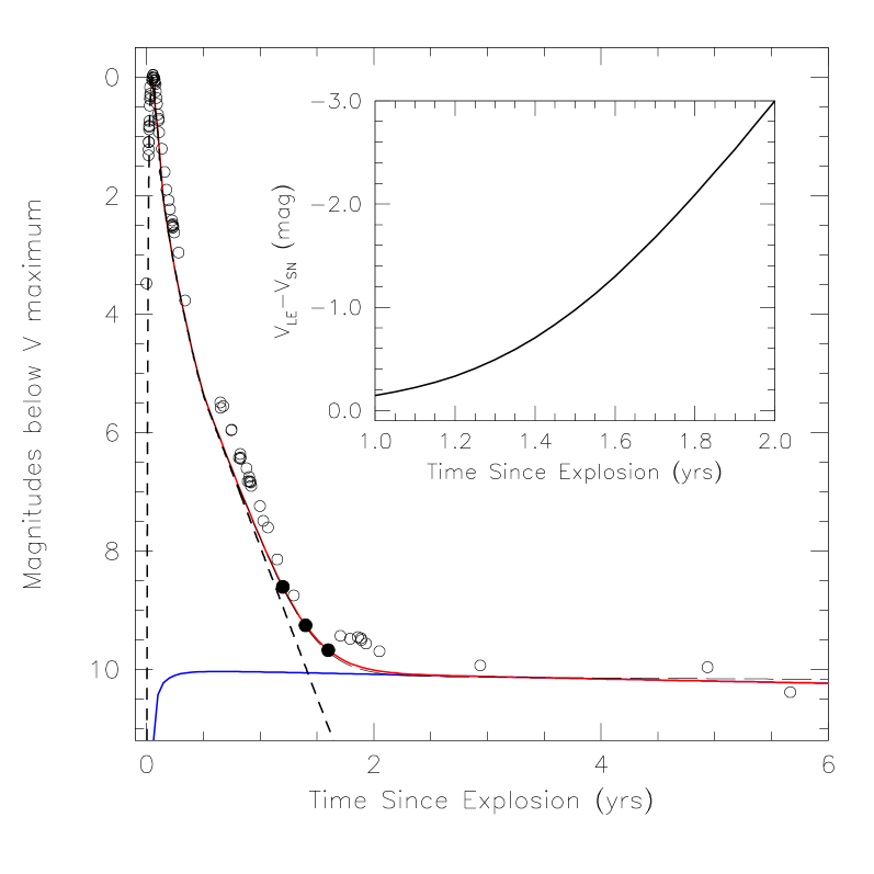
Figure 5: Light curve calculated for a perpendicular sheet with a thickness $\Delta R$=50 lyr placed in front of the SN with $D$=200 lyr and $n_{H}$=5 cm^-3 ($\tau_{d}(V)$=0.12, solid line) and $D$=800 lyr and $n_{H}$=40 cm^-3 ($\tau_{d}(V)$=0.99, long-dashed line). The short-dashed line traces the exponential decay of the template light curve, the circles are the observed data for SN 1991T (Schmidt et al., 1994; Sparks et al., 1999) and filled dots mark the phases 1.2, 1.4 and 1.6 yr. The insert shows the deviation of the measured magnitude from the radioactive decay tail for the first geometry.

4 Effects on SN spectra and light curves

Using the library we have presented here and the SSA approximation (or the Monte Carlo approach when required) discussed in Paper I, we have computed the LE spectra and analyzed the effects these have on objects like SNe 1992A and 1994D under two very different conditions, i.e. when the dust cloud is very large ($t_{c}\geq t$) and in the opposite case when its size is very small ($t_{c}\ll t$).

4.1 Case A: large clouds ($t_{c}\geq t)$

To illustrate the LE effects in the large cloud case (see Fig. 1, left panel), we run a series of calculations using the SSA approximation and a simple dust geometry, placing a dust sheet perpendicular to the line of sight at $D$=200 lyr in front of the SN, with a thickness $\Delta R$=50 lyr and a particle density $n_{H}$=5 cm^-3. This configuration, which implies $\tau_{d}(V)$=0.12 (or $A_{V}$=0.13) produces a light curve which is qualitatively similar to what was observed in 1991T (Schmidt et al., 1994; Sparks et al., 1999), as shown in Figure 5. We remark that we did not make any special attempt to fit the SN 1991T data since our purpose here is to show the general effects in a realistic situation. In this respect, it is also worth mentioning that the light curve of this slow declining object and its spectra at maximum where rather different from those we have used for our calculations (see for example the broad light curve peak shown by 1991T in comparison to our template in Figure 5). A more detailed analysis of the SNe 1991T and 1998bu cases is going to be presented in a separate paper.

As shown in Figure 5, the light curve starts to deviate from the ordinary exponential decay (dashed line) at about one year after the explosion, to settle down on a very slow decline, totally driven by the LE, at about two years past the explosion. Between these two extremes, the observed spectrum is expected to show a gradual transition from that typical of a Ia at late phases to that of a pure LE.

The amount of the LE contamination can be judged in Figure 6, where we have plotted the results for $t$=1.2, 1.4 and 1.6 yr from the explosion. Already at the first epoch, when the total $V$ luminosity (SN+LE) is only 0.2 mags brighter than that expected for the radioactive decay, the resulting spectrum is sensibly different from that of a Ia at these phases, especially in the blue. Due to the peak present in the LE spectrum at about 4600Å, the most prominent feature of the intrinsic nebular SN spectrum at 4700Å, normally attributed to [FeIII], appears to be broadened and the region between 4000 and 4500 Å much bluer than in an unaffected Ia. This is actually quite similar to what was seen in SN 1998bu (Spyromilio et al., 2004) in the spectrum obtained 381 days past $B$ maximum (see also Figure 4 here), where the bump at about 4000 Å is unusually bright.

Figure 6: Evolution of the global spectrum (SN+LE, thick curve) at three different epochs for the model described in the text. The dashed line traces the LE spectrum while the dotted line is the SN spectrum reddened by $A_{V}$=0.13. For presentation, SN and global spectra have been normalized to their maxima.

Figure 7: Light curve calculated with the MC code for the $r^{-2}$ wind with $R_{0}$=0.01 lyr. The curves trace the global (SN+LE, thick) and extincted SN (thin) light curves for $\tau_{d}(V)$=0.5 (solid) and $\tau_{d}(V)$=3.0 (dashed). The insert shows the deviation of the global light curve (SN+LE) from the SN light curve for the two optical depths. As a guide for the eye, the vertical dashed-dotted line marks the position of $V$ maximum.

The consequences of a LE in the red are milder, and tend to emerge only at later phases. The dominant [FeIII] bump gets gradually fainter compared to the other emerging features and the colour becomes bluer and bluer, reaching $(B-V)\simeq-$0.2 when the spectrum is totally dominated by the LE, around 2 yr after the explosion. During the transition phase a distinguishing feature is also the appearance of CaII H&K lines, reflecting their strong presence in maximum light spectra.

The outcome can be different if the dust optical depth is increased, mainly due to the LE self absorption (see Paper I). To illustrate this fact, we have run a series of calculations placing the dust sheet at $D$=800 lyr and increasing its optical depth to $\tau_{d}(V)$ to about 1 ($n_{H}$=40 cm^-3). The distance was properly tuned to produce a LE with the same observed magnitude as the one discussed earlier (see Figure 5, long-dashed line). In this case the LE spectrum is much redder, having $(B-V)\sim$+0.15. As a matter of fact, both the SN and the LE undergo roughly the same reddening, which in this case is $E(B-V)\simeq$0.35.

In general, for higher extinctions the SSA approximation becomes insufficient and a more complicated multiple scattering approach has to be performed (see Paper I).

Before moving to the next section we like to make a consideration on the late spectrum shown by SN 2001el. Besides the intense bump at about 7500Å, the region between 4200 and 5400Å appears to be rather blue. In particular, the bump at 4400Å is much more intense than in any of the other objects presented in Figure 4. The synthetic colour of the observed spectrum is $(B-V)$=0.25, and it reduces to $(B-V)$=0.07 after applying the extinction reported by Krisciunas et al. (2003) for $R_{V}$=3.1. This value is unusually blue when compared to the ones derived from the spectra of SN 1994D (0.38) and SN 1992A (0.34).

Figure 8: Same as Figure 9 for $\tau_{d}(V)$=3.0 ($A^{0}_{V}$=3.26).

At a first glance this might be interpreted as the signature of an underlying LE, but there are two quite important aspects that need to be considered. The first is that the synthetic magnitude deduced from the observed spectrum is $V$=21.24, which is in perfect agreement with the standard luminosity decline. Secondly, the spectrum drops quite fast below 4300Å, contrarily to what happens for instance to 1998bu (see Figure 4). The simulations show that changing the optical depth of the region which is responsible for the hypothetical LE does not allow to produce the drop which is seen in the blue. The conclusion is that the late time spectral appearance of SN 2001el is not caused by a LE of the type considered in this section.

In general, when the dust region is sufficiently extended in the direction perpendicular to the line of sight, the dust system integrates the emitted SN spectra over the whole time range from the explosion to the epoch of the observation ($t_{c}\geq t$), so that the resulting LE spectrum is very different from that of the SN at any given epoch. Therefore, it is very easy to detect its emergence, that can be difficultly mistaken with intrinsic features. An increase in the dust density would simply anticipate the time when the LE emerges, change the colour of the LE itself and cause a larger extinction on the SN itself, but the LE characteristic spectral features will still be very well pronounced.

4.2 Case B: small clouds ($t_{c}\ll t$)

Figure 9: Evolution of the global spectrum (SN+LE, thick curve) at four different epochs for the wind model with $R_{0}$=0.01 lyr and $\tau_{d}(V)$=0.5. The dashed line traces the LE spectrum while the dotted line is the SN spectrum reddened by $A^{0}_{V}$=0.54. For comparison, the latter spectrum has also been scaled to match the integrated flux of the global spectrum (SN+LE, thin solid line).

Table 1: LE effects on a $r^{-2}$ dust distribution for three different values of the inner wind boundary $R_{0}$ (see text). All values are in mag, with the exception of $\gamma(B)$ (mag/100^d) and $\Delta t_{max}$ (days). The number under the labels of columns 4, 5 and 6 indicate the reference values for the input light curve. The meaning of each column is explained in the footnotes.

$\tau_{d}(V)$	$A^{0}_{V}$	$E^{0}(B-V)$	$\Delta m_{15}(B)$	$\gamma(B)$	$\Delta m_{300}(B)$	$\Delta t_{max}$	$\Delta V_{max}$	$\Delta(B-V)_{max}$	$E(B-V)_{max}$	$A_{V}$	$A^{\prime}_{V}$	$\Delta M_{V}$
			[1.45]	[1.40]	[6.98]
$R_{0}$=0.1 lyr
0.1	0.11	0.04	1.36	1.29	6.70	0.0	$-$0.02	$-$0.01	0.03	0.09	0.08	+0.01
0.5	0.54	0.18	1.16	1.10	5.91	1.2	$-$0.10	$-$0.05	0.13	0.44	0.40	+0.04
1.0	1.09	0.35	0.95	1.01	5.23	2.6	$-$0.24	$-$0.07	0.29	0.84	0.88	$-$0.04
2.0	2.17	0.70	0.55	0.93	4.29	3.4	$-$0.48	$-$0.16	0.54	1.69	1.68	+0.01
3.0	3.26	1.05	0.30	0.89	3.65	4.8	$-$0.75	$-$0.25	0.80	2.52	2.48	+0.04
$R_{0}$=0.01 lyr
0.1	0.11	0.04	1.38	1.41	6.94	0.0	$-$0.05	$-$0.02	0.02	0.05	0.05	$-$0.00
0.5	0.54	0.18	1.30	1.43	6.79	1.2	$-$0.27	$-$0.09	0.09	0.28	0.28	$-$0.00
1.0	1.09	0.35	1.24	1.43	6.63	2.6	$-$0.56	$-$0.14	0.21	0.53	0.64	$-$0.11
2.0	2.17	0.70	0.97	1.37	6.31	3.2	$-$1.07	$-$0.28	0.42	1.10	1.29	$-$0.19
3.0	3.26	1.05	0.86	1.33	6.04	4.4	$-$1.56	$-$0.41	0.64	1.70	1.99	$-$0.29
$R_{0}$=0.005 lyr
0.1	0.11	0.04	1.41	1.41	6.96	0.0	$-$0.06	$-$0.02	0.02	0.00	0.05	$-$0.00
0.5	0.54	0.18	1.39	1.45	6.88	1.1	$-$0.30	$-$0.09	0.08	0.24	0.25	$-$0.01
1.0	1.09	0.35	1.29	1.48	6.78	1.5	$-$0.60	$-$0.17	0.18	0.49	0.55	$-$0.06
2.0	2.17	0.70	1.19	1.49	6.60	2.8	$-$1.17	$-$0.30	0.40	1.00	1.23	$-$0.23
3.0	3.26	1.05	1.03	1.47	6.46	3.1	$-$1.69	$-$0.44	0.61	1.57	1.90	$-$0.33
$A^{0}_{V}$=1.086$\tau_{d}(V)$; $E^{0}(B-V)$=$A_{V}^{0}$/3.1; $\Delta m_{15}(B)$=$B_{15}-B_{max}$; $\gamma(B)$=$(dB/dt)_{t>180}$; $\Delta m_{300}(B)$=$B_{300}-B_{max}$; $\Delta t_{max}$=$t_{max}-t^{0}_{max}$;
$\Delta V_{max}$=$V_{max}-V_{max}^{0}+A^{0}_{V}$; $\Delta(B-V)_{max}$=$(B-V)_{max}-(B-V)^{0}_{max}+E^{0}(B-V)$; $E(B-V)$=$E^{0}(B-V)+\Delta(B-V)_{max}$;
$A_{V}$=$A_{V}^{0}+\Delta V_{max}$; $A^{\prime}_{V}$=3.1$E(B-V)$; $\Delta M_{V}$=$A_{V}-A^{\prime}_{V}$.

More subtle is the case when the dust system characteristic dimension is significantly smaller than $ct$ (see Fig. 1, right panel). In fact, under these conditions, the dust system integrates the SN input spectra over times which are much shorter than the time elapsed from the explosion (i.e. $t_{c}\ll t$) and the resulting LE spectrum is much closer to the SN spectrum, making it very difficult to detect it on the basis of the spectral appearance alone. Of course, in order to have this effect, the dimension of the dust cloud must be indeed small. For example, for a spherical dust cloud with radius $R$ and centered on the SN it is easy to show that $t_{c}=2R/c$. The simulations show that in order to have a LE spectrum which is very similar to that of the SN at all epochs, one needs to have $t_{c}\leq$0.2 lyr, which implies $R\leq$0.1 lyr ($\sim$10¹⁷ cm). Since these dimensions are much smaller than those of typical interstellar dust clouds, the most natural scenario to be considered is the one of circumstellar material. As done by Chevalier (1986), Patat (2005) and Wang (2005), we will consider here the simplest case, i.e. that of a spherically symmetric stellar wind in which the density is given by $n(r)=n_{0}(R_{0}/r)^{2}$, where $R_{0}$ is the inner boundary of the wind, within which the density is supposed to be null. Also, we assume that the wind has an outer boundary, defined by $R_{1}>R_{0}$. Under these circumstances, the optical depth along the line of sight is simply $\tau_{d}=C_{ext}\;n_{o}\;R_{0}\;(1-R_{0}/R_{1})$, from which it is clear that if $R_{1}\gg R_{0}$ the value of $\tau_{d}$ is practically independent from $R_{1}$. As we have shown in Paper I (cf. Fig. 6) this geometry, compared to the others we had explored, is able to produce quite bright LEs with a fast declining light curve.

To illustrate the effects of such a dust geometry, we have run a series of calculations using the MC code we have described in Paper I. In all simulations we have used the canonical Milky Way dust mixture with $R_{V}$=3.1 (Draine, 2003) and we have computed the LE $B$ and $V$ light curves and optical spectra for $R_{0}$=0.1, 0.01 and 0.005 lyr, keeping $R_{1}$=1.0 lyr and for different values of $\tau_{d}(V)$ (0.1, 0.5, 1.0, 2.0 and 3.0). Two examples of the resulting curves are presented in Fig. 7 for $R_{0}$=0.01 lyr and $\tau_{d}(V)$=0.5, 3.0. The main photometric parameters obtained from the global light curves (SN+LE) are summarized in Table 1, where besides the the optical depth and the implied extinction and colour excess ($\tau_{d}(V)$, $A^{0}_{V}$ and $E^{0}(B-V)$) we show the usual $\Delta m_{15}(B)$, the slope at phases later than 6 months ($\gamma(B)$), the magnitude jump between maximum and 300 days past maximum ($\Delta m_{300}(B)$), the time shift in the $B$ maximum ($\Delta t_{max}$), the differences in $V$ and $(B-V)$ at maximum with respect to the extincted SN ($\Delta V_{max}$, $\Delta(B-V)_{max}$), the colour excess with respect to the unreddened SN at maximum ($E(B-V)_{max}$), the apparent extinction obtained comparing with the intrinsic magnitude ($A_{V})$, the extinction derived from $E(B-V)_{max}$ assuming $R_{V}$=3.1 ($A^{\prime}_{V}$) and the deviation of the absolute magnitude at maximum with respect to the input value ($\Delta M_{V}$). For comparison, the corresponding values for the template light curves assumed by the models are as follows: $\Delta m_{15}(B)$=1.45 mag, $\gamma(B)$=1.40 mag/100^d and $\Delta m_{300}(B)$=6.98 mag.

There are several conclusions that can be drawn already inspecting Table 1. First of all, as already qualitatively noticed by Wang (2005), the resulting light curves become broader and the maximum is attained later then in the pure SN case (cf. also Fig. 7). This has the clear effect of decreasing $\Delta m_{15}(B)$ rather sensibly and the change increases with $\tau_{d}(V)$ and $R_{0}$. Moreover, the global colour gets bluer than that of the purely extincted SN and this effect becomes stronger for larger $\tau_{d}$ and smaller $R_{0}$. In principle, unless the values of this parameters become too deviant from the normal ones (0.9 $\leq\Delta m_{15}(B)\leq$1.9, Phillips et al. 1999), they could be attributed to an intrinsic feature of the SN. Nevertheless, there are other side effects that tend to betray the presence of an underlying LE. In fact, the late time decay rate $\gamma(B)$ increases with $\tau_{d}$ and $R_{0}$, while the magnitude jump $\Delta m_{300}(B)$ grows with $R_{0}$ and decreases for increasing values of $\tau_{d}$. In the case of $R_{0}$=0.005 lyr ($\sim$5$\times$10¹⁵ cm), the global light curve around maximum light changes but its overall shape remains similar to the template light curve (e.g. giving plausible values for $\Delta m_{15}(B)$, $\Delta m_{300}(B)$ and so on). This has a very interesting consequence, at least for $R_{0}\leq$0.01 lyr. In fact, besides measuring a slower post-maximum decline rate, one would also measure a colour which is significantly bluer and a global apparent luminosity which is higher than those of the purely reddened SN. As the simulations show, these two facts combined together would lead an hypothetical observer deducing the reddening correction from the global observed colour (and using a standard value for $R_{V}$) to derive an absolute luminosity which is brighter than the real one by an amount that can reach about 0.3 mag (see last column of Tab. 1). In conclusion, one would attribute the smaller value of $\Delta m_{15}(B)$ to a larger intrinsic luminosity, as in the case of the classical Phillips relation (Phillips et al., 1999). Of course this does not mean that the observed relation is produced by dust in the vicinity of the SN, since $\Delta m_{15}$ correlates in fact with other features like spectral line ratios (Nugent et al., 1995; Benetti et al., 2005; Hachinger, Mazzali & Benetti, 2005; Bongard et al., 2005). But certainly, the presence of hidden LEs might introduce an additional spread in the measured photometric parameters.

The effects on spectra are presented in Fig. 9 and 8, where we show the time evolution in the $R_{0}$=0.01 lyr case for $\tau_{d}(V)$0=0.5 and 3.0. In the low optical depth case the effect is rather mild (the global spectrum is slightly bluer than that of the reddened SN spectrum at all phases), while the LE influence becomes much more relevant in the high optical depth case. As a consequence of the increased LE contribution to the total flux, the time integration becomes visible and this causes the spectral features to show clear deviations from the intrinsic ones. The most remarkable is the absorption profile of the Si II 6355 Å line around maximum light ($t$=0.05 lyr), which is much broader. The same behaviour is shown by all lines and at all epochs. A late phases, the line peaks also appear blue-shifted with respect to the intrinsic features. Moreover, as in the low density case, the global spectrum is bluer than the reddened SN spectrum at all times.

In general, the strongest effect is expected around maximum light and in the weeks that immediately follow it, i.e. when the spectral evolution is fast compared with the LE integration time which, in the case of $R_{0}$=0.01 lyr is of the order of 12 days. In the pre-maximum phase, the early spectra contribute quite marginally to the global flux, due to the very rapid rise in luminosity while, just after maximum, the SN flux in the preceding days is actually higher than on the current epoch, so that the contribution is indeed relevant. This is clearly displayed in Fig. 10, where we present the calculated evolution of the Si II region between $t$=0.03 and $t$=0.10 yrs, which correspond to $-$7.3 and +18.3 days past maximum light. On the first epoch, the profile of the global spectrum is already broader than in the input SN, but the deviation grows in the following days, reaching a maximum during the two weeks past maximum light. The position of the absorption through minimum appears to be red-shifted with respect to the input spectrum, producing a lower photospheric velocity estimate. During the second week, also the emission peak of the line is affected and it appears much broader, reflecting the higher velocities reached in the preceding epochs. These deviations, together with those shown by the light (and colour) curves, would most probably allow one to recognize the presence of a LE. Nevertheless, we must notice that this is true only for high optical depths, while for $\tau_{d}(V)\leq$1, the effects on photometric parameters and spectral features are rather mild (see Table 1 and Fig. 9), making the detection of the LE certainly much more difficult. In those cases the net effect of the LE would be to alter the colours and the overall flux of the observed spectrum, with the consequences discussed by Wang (2005), that we will analyze in the next section.

5 Implications on extinction and extinction law

If a SN is affected by the emergence of a LE, it is clear that each time one tries to derive the amount of extinction or information about the dust properties, the results will be in general misleading. As we have done in the previous section, we distinguish here the two opposite cases.

5.1 Case A

When Schmidt et al. (1994) discovered the LE in SN 1991T, they noticed that, in order to reproduce the observations, they had to correct the time integrated SN spectrum $\cal S$ for the effects of scattering. These were parameterized with a function of the type $\lambda^{-\alpha}$ and the best fit was obtained using $\alpha$=2. As we have seen in Section 2, the correction one has to apply to $\cal S$ includes three components: the first is related to the light scattered by the dust into the observer’s line of sight (directly proportional to $C_{ext}$), the second accounts for the reddening suffered by the SN (proportional to $e^{C_{ext}}$) while the third describes the auto-absorption within the dust cloud that generates the LE itself (proportional to $e^{-C_{ext}})$. Finally, there is a mild wavelength dependency introduced by the albedo and a more important contribution by the function $G(\lambda,t)$ (see Section 2). A more convenient formulation can be obtained passing from the extinction cross section $C_{ext}(\lambda)$ to the normalized extinction law $a(\lambda)$. If we pose

$$a(\lambda)=\frac{C_{ext}(\lambda)}{C_{ext}(V)}$$

then the absorption (in magnitudes) can be expressed as $A(\lambda)=a(\lambda)A_{V}$ and equation (4) can be rewritten as

$$\frac{S_{LE}(\lambda,t)}{{\cal S}(\lambda,t)}\propto G(\lambda,t)\;\omega(\lambda)\;a(\lambda)\;e^{\frac{\kappa(V)\;a(\lambda)}{1.086}}$$ (5)

where $\kappa(V)=A_{d}(V)-A_{eff}(V)$ is expressed in magnitudes. In a first approximation, one can parameterize $a(\lambda)$ with a power law of the type $\lambda^{-\beta}$. From equation (5) it is clear that a fitting to the ratio between $S_{LE}$ and ${\cal S}$ using a power law $\lambda^{-\alpha}$ would give a value for $\alpha$ which is not directly related to $\beta$, since other terms with different wavelength dependencies enter its expression. In fact, using our simulations for the perpendicular sheet with $D$=200 lyr we have found that for the Milky Way dust mixture with $R_{V}$=3.1 (Draine, 2003), the best fit values of $\alpha$ depend mostly on the value of $\kappa(V)$, while the dependence on $\tau_{eff}$ is very mild, at least in the validity range of the SSA approximation ($\tau_{eff}\leq$1). Typical values for $\alpha$ are 1.4, 1.7, 2.0 and 2.2 for $\kappa(V)$=$-$0.2, 0.0, 0.2 and 0.4 respectively.

Figure 10: Evolution of the Si II 6355Å region for $R_{0}$=0.01 lyr and $\tau_{d}(V)$=3.0 between $-$7.3 to +18.3 days past maximum light. The dotted curves trace the reddened SN spectra. For presentation they have been scaled by a suitable amount in order to match the global spectrum. The vertical dashed line marks the position of the absorption minimum of Si II in the first spectrum. In the MC simulations the photons where collected with a resolution of $\Delta\lambda$=15 Å and a time bin $\Delta T$=0.01 yrs.

It is interesting to notice that the $\alpha$=2 value found by Schmidt et al. (1994) can be explained with a canonical extinction law and a small difference between the extinction suffered by the LE and the SN, i.e. only 0.2 mag. The SN was certainly reddened: Phillips et al. (1999) report in fact a total extinction $A_{V}$=0.53$\pm$0.17, 0.46 of which is due to the host galaxy. If we assume $A_{d}$=0.46 (or equivalently $\tau_{d}(V)$=0.42) we can therefore give an estimate to $A_{eff}$, which turns out to be 0.26 (i.e. $\tau_{eff}(V)$=0.24). The corresponding model is presented in Figure 11. Given the fact that the synthetic spectrum has been computed using the spectra of objects like 1994D and 1998aq which are quite different from SN 1991T, especially during the maximum light phase, the match is reasonably good. However, we must notice that the observed spectrum is also compatible with $\kappa(V)$=0, i.e. with the SN and the LE suffering the same amount of reddening (Figure 11, thin smooth curve).

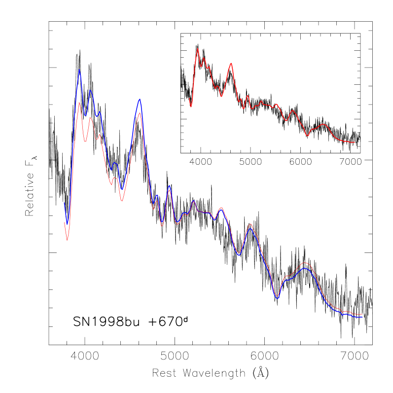
Figure 14: Spectrum of SN 1998bu at 670 days past $B$ maximum (Cappellaro et al., 2001). The spectrum was corrected for the Milky Way reddening ($A_{V}$=0.08, Jha et al. 1999). The smooth curves are synthetic LE spectra with $\tau_{eff}$=0.62 (thick) and $\tau_{eff}$=0.90 (thin) respectively. The upper right insert shows the results for the same dust sheet placed at $D$=0 and $\tau_{eff}$=0.25 ($A_{V}$=0.27).

Another example of a possibly similar situation is given by SN 1998bu. Cappellaro et al. (2001) have presented a LE spectrum at 670 days past maximum light, with a $(B-V)$ colour close to 0, i.e. very similar to that observed for SN 1991T (Schmidt et al., 1994). On the other hand, Jha et al. (1999) have reported a total extinction $A_{V}$=0.94 $\pm$0.15, while Hernandez et al. (2000) found $A_{V}$=1.0 $\pm$0.1. Using the same geometrical configuration, the best fit with the observed LE spectrum is obtained for $\tau_{eff}(V)$=0.62, which implies $A_{V}$=0.67 (see Figure 14). Given the fact that the estimated galactic extinction in the direction of SN 1998bu is only $A_{V}$=0.08 (Schlegel, Finkbeiner & Davis, 1998), this value is about 0.2 mag lower than the average value reported by Jha et al. (1999) and Hernandez et al. (2000).

In this respect it is interesting to note that, due to the geometrical effect related to forward scattering that we have described in Section 2, if the dust is close to the SN, then a lower dust optical depth would still produce a red LE spectrum. This is not because there is more reddening, but because under these circumstances the scattering efficiency does not grow at shorter wavelengths as fast as it does if the dust is located far way. This is illustrated in the insert of Fig. 14, where we have plotted the results of a simulation where the same perpendicular sheet is placed at distance $D$=0. In this case the best fit is obtained for $\tau_{eff}(V)$=0.25, which would imply a SN extinction $A_{V}$=0.27, which is significantly lower than the values reported in the literature.

In conclusion, the information on the extinction and the extinction law one derives from the observed LE spectrum is geometry dependent and not univocally related to the dust properties.

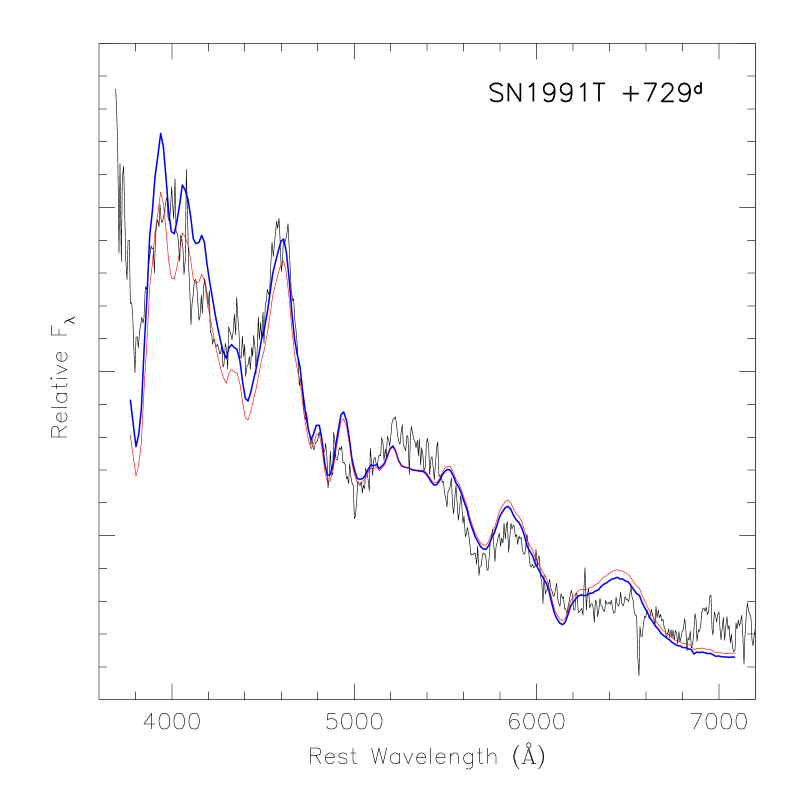
Figure 11: Spectrum of SN 1991T at 729 days past $B$ maximum (ESO Key Programme). The spectrum was corrected for the Milky Way reddening ($A_{V}$=0.07, Phillips et al. 1999). The thick smooth curve is a synthetic LE spectrum obtained with the spectral library described in the text with $\tau_{eff}$=0.24. For comparison, a synthetic spectrum with $\tau_{eff}$=0.42 is also shown (thin curve).

5.2 Case B

As we have seen in Sec. 6, the presence of a LE produced by a dust geometry with $t_{c}\ll t$ is able to introduce sensible luminosity and colour changes with mild effects on the other photometric and spectroscopic characteristics, provided that $\tau_{d}(V)\leq 1$. This, as Wang (2005) has shown, can have an interesting consequence on the properties one would deduce for the dust. In fact, if we take the example of $R_{0}$=0.01 lyr and $\tau_{d}(V)$=1.0, from Table 1 we see that, due to the presence of a LE, the global $V$ magnitude is 0.56 brighter than the purely extincted SN, which is affected by an extinction of $A^{0}_{V}$=1.09 mag. Therefore, assuming a distance to the SN and using the expected absolute luminosity, one would deduce $A_{V}$=0.53. Then, comparing the colour at maximum with a reference value (which here we assume to be the one of our template object), one would also deduce $E(B-V)_{max}$=0.21 from which she would erroneously conclude that $R_{V}\sim$2.5. As far as the photometric properties are concerned, such an object would show normal $\Delta m_{15}(B)$ (1.24) and $\gamma(B)$ (1.43) and at late phases the slight over-luminosity (0.3 mag) would probably go unnoticed due to the measurement errors. Therefore, at least on the basis of those parameters, it would be very difficult to recognize the presence of an underlying LE.

Since the difference between the global luminosity and that of the pure SN is not constant in time and changes rather rapidly around maximum light (see Fig. 7, upper right insert), the values of $R_{V}$ deduced in this way are expected to change with time in a similar way. This is illustrated in Fig. 12, where we present the results of MC simulations for $R_{0}$=0.01 lyr and two different values of the dust optical depth. The total-to-selective absorption ratio changes in fact very rapidly from the explosion to about 0.15 yrs, which correspond to the maximum of the intrinsic SN ($B-V)$ colour curve (dotted curve). After that epoch, the ratio remains almost constant. This behaviour is qualitatively similar to the one found by Wang (2005) (see his Fig. 2) and the discrepancies are probably due to the different treatments of multiple scattering.

It is important to remark that the global colour curve is not obtained by a simple rigid reddening of the unextincted SN colour curve. On the contrary, the difference between bluest and reddest colour is smaller and the tail at phases later than 0.15 yrs ($\sim$55 days) is less steep. The effect becomes more pronounced for higher optical depths. In other words, once the observed global colour curve is corrected for the colour excess deduced at maximum, this is not going to match a reference colour curve and the late behaviour would clearly differ from the homogeneous trend found by Lira (1995). We reckon that this colour effect, shown also by the semi-analytical calculation of Wang (2005) (see his Fig. 3, lower panel) is a good diagnostic to unveil the presence of a hidden LE.

Figure 12: Upper panel: colour evolution for the wind dust geometry with $R_{0}$=0.01 lyr for $\tau_{d}(V)$=1.0 (lower thick curve) and $\tau_{d}(V)$=3.0 (upper thick curve). The dashed lines trace the corresponding colour curve in the case of pure extinction and $R_{V}$=3.1, while the dotted curve is the SN intrinsic colour. Lower panel: ratio between $A_{V}=V-V^{0}_{SN}$ and $E(B-V)_{max}$ deduced comparing the global colour with the intrinsic colour of the SN at maximum for $\tau_{d}(V)$=1.0 (solid line) and 3.0 (dashed line). The insert shows the behaviour of $A_{V}$ in the two cases. In all plots the vertical dotted line marks the epoch of maximum light.

At this point we must emphasize that, in all practical cases, the colour excess is deduced from the data using the colour curve. On the contrary, the extinction is usually derived from this value after assuming $R_{V}$ and then applied to the observed magnitude to obtain the absolute luminosity of the object (see for example Benetti et al. 2004). Following this procedure in the case of our previous example would lead to a result which is actually not far from the real one. In fact, if one adopts $E(B-V)$=0.21 and assumes $R_{V}$=3.1, this would produce an absolute magnitude which is only 0.11 mag brighter than the real value (see Table 1, last column). Remarkably, this is of the same order of the correction foreseen by the Phillips relation (Phillips et al., 1999) for the given $\Delta m_{15}(B)$. As we had already noticed in Sec. 6, this effect is most likely going to add a spread to the observed luminosity-decline rate relation.

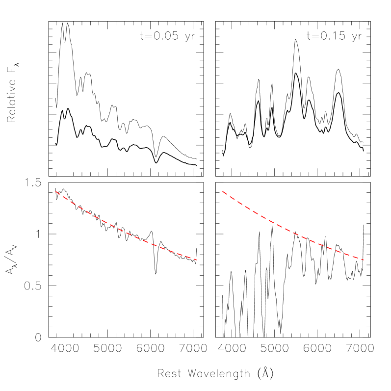
Figure 13: Upper panels: comparison between the global spectrum (thick curve) and the intrinsic SN spectrum (thin curve). Lower panels: comparison between intrinsic ($R_{V}$=3.1, dashed curve) and derived (solid curve) normalized extinction laws. The simulations were performed using $R_{0}$=0.01 lyr and $\tau_{d}(V)$=1.0.

Another way of deriving information on the extinction law $A(\lambda)$ is to compare the observed spectrum $S(\lambda)$ with a reference unreddened SN spectrum $S^{0}(\lambda)$ obtained at the same phase and corrected to the same distance (see for instance Elias-Rosa et al. 2005). If the LE effects were negligible, one could in fact write $A(\lambda)=1.086\;\ln[S^{0}(\lambda)/S(\lambda)]$ and hence derive directly the extinction wavelength dependency. Of course, when $S(\lambda)$ contains a significant contribution from the LE the result is going to be misleading. This is clearly illustrated in Fig. 13, where we present the results obtained from our Monte Carlo simulations at two different epochs ($t$=0.05 and 0.15 yrs) for the case $\tau(V)$=1.0 and $R_{0}$=0.01 lyr. For the first epoch, which approximately corresponds to the $B$ maximum light, the colour of the global spectrum is clearly redder than that of the unreddened SN ($E(B-V)\sim$0.2, see also Fig. 12) and the derived extinction law is just slightly steeper than the input one, thus giving a smaller $R_{V}$. With the exception of the SiII 6355Å feature, the derived curve is reasonably smooth. Totally different is the case at $t$=0.15, which roughly corresponds to the maximum of the $(B-V)$ colour curve. At this phase, in fact, the colours of the global spectrum and the unreddened SN are similar (see also Fig. 12) and the derived extinction law is dominated by the differences displayed by the two spectra due to the time integration effects. Of course, in a real case, this could be interpreted as the presence of a LE but also with a deviation from the standard spectral evolution. Irrespective of the physical reason, the apparent evolution shown by the derived extinction law is a clear diagnostic signaling that additional effects are present and that $R_{V}$ can not be estimated with this method. Given these facts, a detailed analysis of extincted Ia should be able to clarify whether this mechanism is indeed at work and whether it can explain the low values of $R_{V}$ derived by several authors.

6 Discussion

All known cases of LEs in Type Ia SNe have revealed themselves through the gradual appearance of an additive flux, during the nebular phase, in the spectral region bluewards of 4500Å, where one can easily recognize the imprints of the time integrated SN spectrum. Therefore, they are instances of the Case A we have described in Sec. 4.1. The spectrum discussed by Spyromilio et al. (2004) is a very good example of this behaviour (see also Figure 4 here). Moreover, due to the close wavelength coincidence of the dominating [Fe III] nebular feature with the most prominent bump of a LE spectrum, the former line is broadened. Besides this, a distinguishing spectral feature of a LE is the clear presence of the Ca II H&K lines which, though, at the beginning of the transition phase can be masked by the presence of a similar structure observed in pure nebular spectra at about 4000 Å.

In general it is fairly easy to recognize the Case A LE contamination on the basis of the late spectra alone, especially if the optical depth is not too high, so that its spectrum is definitely blue, with $(B-V)\leq$0. In cases where the LE forms in regions of high dust density, its spectrum can turn red without necessarily having the SN spectrum reddened. In this case, the LE contamination is a bit more subtle and tends to leave unchanged the overall colour of the observed spectrum. However, the characteristic LE bumps at about 5900Å and 6500Å (see Figure 6) appear quite clearly.

An interesting fact that emerges from the analysis of the two known cases of SNe 1991T and 1998bu when compared to our synthetic LE spectra is that clear differences are visible. As far as 1991T is concerned, its LE dominated spectrum taken at 729 days past maximum (cfr. Figure 11) shows interesting features, which are directly related to its peculiar appearance during the maximum phase (see for instance Filippenko et al. 1992). In particular, we notice that the absence of the distinguishing Ia feature (i.e. the Si II 6150 Å) during the pre maximum phase and its weakness in post maximum is reflected in the LE spectrum. In fact, while our synthetic spectra, calculated using “normal” events like SNe 1994D and 1998aq, do show a clear imprint of the P-Cyg profile displayed by this line during the photospheric phase, this is practically absent in the data of 1991T. Another clear difference is that visible in correspondence of the CaII H&K lines. Again, the weakness of this feature in 1991T is a consequence of what happened in the pre-maximum phase, when this line was totally absent (Filippenko et al. 1992).

In the other case, the match between the synthetic and the observed LE spectrum is fairly good but, still, the observed deviations can all be attributed to small differences in the spectral appearance of SN 1998bu with respect to SN 1994D (see Hernandez et al. 2000).

All of this has an interesting consequence, i.e. that the maximum phase peculiarities can be easily seen in the LE spectrum. Therefore, not only one could classify an historical SN on the basis of its LE spectrum alone (disentangling for example between a Type I and a Type II), but one could also get some more detailed information about its features during maximum light, so that it would be possible to distinguish, for instance, between a normal Ia, a 1991T-like or a 1991bg-like event. This might have some relevance when traces of an historical SN explosion are found by detecting its LEs, as in the recent cases near the SN remnant of Cas A (Krause et al., 2005) and in LMC (Rest et al., 2005). Provided that the LE is bright enough to allow a spectroscopic observation, this would provide a powerful tool to type the SN. The detections by Krause et al. (2005) and Rest et al. (2005) lets us hope that more cases will be discovered in connection with SN remnants in our Galaxy, offering a unique chance to directly classify the explosion that generated them and to establish a firm connection between the two.

In principle one could envisage to use the Case A LE observations to derive some information about the extinction law in the host galaxy, simply comparing the SN time integrated spectrum and the LE spectrum. In fact, under the conservative assumption that the LE and the SN suffer the same extinction (i.e. $\kappa(V)$=0 in equation (5)), the ratio between $S_{LE}$ and $\cal S$ is reddening independent. Unfortunately, even in these simplified circumstances, one is left with the albedo and forward scattering degree wavelength dependence. More in general, due to the way the effects of geometry, optical depth and dust properties combine together, one cannot derive unambiguous information on the extinction law since very similar solutions can be obtained using different ingredients. Some meaningful results might be achievable from spectroscopic observations of LEs if some of the dependencies can be removed by other and independent observations. Of great help, in this respect, are high spatial resolution images, which can give direct information on the geometrical dust distribution.

With the increased interest on Type Ia SNe related to their usage in cosmology and the availability of larger and larger observing facilities, it is most likely that an increasing number of objects belonging to this class will be observed in the near future and followed up to even more advanced phases than it is currently done. Our forecast is that these investigations will probably be disturbed by the presence of LEs, too faint to be detected by the typical current instrumentation. In fact, as we have shown here, a dust density of the order of $n_{H}$=5 cm^-3 is sufficient to produce a LE compatible with those seen in SNe 1991T and 1998bu. Due to the lack of LE detections in the vast majority of the cases (Boffi et al., 2003), in Paper I we had concluded that the height scale of Type Ia must be significantly higher than that of the dust in the disk of host galaxies. Indeed, a very similar conclusion was reached by Della Valle & Panagia (1992) on the basis of completely independent considerations.

Nevertheless, when one pushes the observations at later phases, due to the fast decay typical of these objects during the nebular phase ($\sim$5 mag yr^-1), the light curve rapidly reaches levels where a LE produced by a much lower densities would dominate the spectrum. For example, for the same geometry used in Figure 5, a density of $n_{H}$=0.5 cm^-3 would produce a LE approximately 2.5 mag fainter, implying that the transition to a LE dominated spectrum would have started only 6 months later. Therefore, the study of Type Ia at phases later than 1.5-2 yr, aimed for example at detecting deviations from the radioactive decay, will be most probably hindered by the emergence of a Case A LE.

If, on the one side, it is true that there is an increasing number of instances where LEs of this kind are actually observed (see also the recent case reported by Sugerman 2005 and Van Dyk, Li & Filippenko 2005 for the core-collapse SN 2003gd), one may in fact wonder whether and to which extent early phases could be affected, modifying for instance the light curve shape, the overall luminosity and introducing peculiarities in the spectral appearance. As we have shown in this paper, this can actually take place when the dust cloud is very close to the SN and has small dimensions, circumstances that we have generically indicated as Case B. As it has been independently shown by Wang (2005), circumstellar dust can in principle alter the observed light and colour curves producing, for example, interesting effects on the derived extinction curve. Our analysis (see Secs. 6 and 5.2), run under the simplifying hypothesis that the dust is distributed according to a $r^{-2}$ law with an inner cavity with radius $R_{0}$, shows that already with moderate optical depths ($\tau_{d}(V)$=1), the presence of dust in the immediate vicinity of a Type Ia ($R_{0}\sim$10¹⁶ cm) would turn into significant changes in the photometric parameters, which would still be within the normally observed ranges. In particular, the post maximum decline rate $\Delta m_{15}$ would be smaller and the SN would also appear inherently brighter, due to the additional flux contribution added by the underlying LE, i.e. producing an additional scatter in the Pskovski-Phillips relation. In this respect, we notice that there are many instances of Type Ia showing low decline rates ($\Delta m_{15}(B)<$1) without displaying the spectral peculiarities typical of slow-declining SN 1991T-like events (see for example Phillips et al. 1999, Table 2).

Besides influencing the photometric parameters, the time integration during the fast evolving phase around maximum light tends to produce changes in the line widths and peaks, altering the measured expansion velocities. As we have said, according to our simulations the deviations from a LE-free standard behaviour would be rather subtle and could be easily misidentified as the intrinsic features of a peculiar object. Whilst most of the photometric parameters tend to be mildly altered (at least for relatively low values of the dust optical depth) the colour evolution shows quite a clear deviation from the homogeneous behaviour shown by Type Ia between 30 and 90 days past maximum light (Lira, 1995). If indeed all LE-free objects follow that path, then the colour curve could be a good diagnostic tool to unveil the presence of a LE.

As pointed out by Wang (2005), the presence of Case B LEs could explain the low values for $R_{V}$ which have been deduced from SN observations (see for example Phillips et al. 1999, Krisciunas et al. 2000, Knop et al. 2003, Altavilla et al. 2004 and Krisciunas et al. 2005 for the most recent examples). As we have shown here, this is in principle true, even though some side effects should be clearly detectable, at least for the simple dust distributions we have analyzed.

According to the lower panel of Fig. 12, or to the equivalent Fig. 3 of Wang (2005), one would expect that the deduced $R_{V}$ remains roughly constant ($\sim$1) in this phase range. Nevertheless, in those plots $E(B-V)$ is kept at the constant value attained at maximum light, while the difference in colour between the global spectrum and the SN spectrum changes with time, both in our Monte Carlo calculations and in the semi-analytical model presented by Wang (2005). In particular, when the global colour becomes equal to or even bluer than that of the unreddened SN, the extinction correction is expected to produce weird results. Therefore, if one attributes the deviations from the standard colours to a different extinction law, she also has to accept the puzzling conclusion that this has to change with time. We reckon that both the colour evolution and the time variability of the derived extinction law would be sufficient to infer that the observed deviations are not due to a peculiar dust composition but rather to a LE.

Another interesting fact worth to be mentioned is the discrepancy that one would find between the extinction derived from the equivalent width of the NaI D lines and that deduced from photometric or spectroscopic comparisons with templates. In fact, while the intensity of the NaI D absorption is related only to the dust present along the line of sight (and would hence give a direct estimate of $\tau_{d}$), all other methods would be affected by the LE contribution. As we have seen in Sec. 5.2, this tends to significantly decrease the amount of derived extinction. In the case of normal dust-to-gas ratios and for a simple $r^{-2}$ spherically symmetric dust geometry, this would imply that the values deduced from the NaI doublet are systematically higher than those inferred from other methods (compare $A^{0}_{V}$ with $A_{V}$ or $A^{\prime}_{V}$ in Table 1).

In all this discussion we have assumed (and required) that there can be dust very close to the SN. In this respect there is a very important consideration one has to make. In fact, if on the one hand it is true that LE effects become more subtle when the dust is closer to the SN (and can therefore be mistaken with intrinsic properties), on the other there actually might be a lower limit for the SN-dust distance. In fact, for typical expansion velocity of 10⁴ km s^-1, the ejecta would reach $R_{0}$=10¹⁶ cm in less than four months. This is a problem that needs to be addressed with detailed modeling, in order to see whether the interaction would be able to destroy and/or sweep away the dust and to evaluate possible effects on the observed reddening, its time evolution and so on. One should also mention that the radiation field produced by the SN explosion would probably evaporate the dust up to a certain radius. If in the case of a core-collapse event the UV flash is expected to produce a cavity in the dust with a radius of $\sim$10¹⁷ cm (see for example Chevalier 1986), the lack of UV photons in a Type Ia might still make the dust survive the explosion. Another implication that needs to be addressed is related to the fact that substantial amounts of dust should be associated with correspondingly high amounts of gas. If the gas is close enough to the SN, then some interaction is expected, like in the case of SN 2002ic (Hamuy et al., 2003).

Finally, what remains to be studied is the effect of asymmetric dust distributions (disks, tori, lobes and so on) that, among other things, would certainly produce a net continuum polarization up to several per cent (see Paper I). Being close to the SN the polarized flux could be in fact high enough to produce detectable effects and serve as a useful diagnostic tool to identify the presence of an underlying Case B LE. Finally, to make the scenario fully self-consistent, one should also investigate the effects of dust heating on IR re-emission, which might turn out to be another observable side-effect produced by this kind of LEs.

Detailed analysis of reddened objects will certainly clarify whether Case B LEs are indeed taking place and this, in turn, will probably give us a few more hints about the nature of Type Ia progenitors. We are currently working on the highly reddened SN 2003cg (Elias-Rosa et al., 2005), which shows clear features that could be interpreted as the signature of a Case B LE. The results will be reported in another paper of this series.

7 Conclusions

In this paper we have analyzed and discussed the effects of LEs on light curves, colours and spectra of Type Ia SNe for two different dust geometries: extended clouds (Case A) and small circumstellar clouds (Case B). The main results can be summarized as follows:

1. The effect of Case A LEs is limited to the late phases. The exact time when the LE contribution dominates the global luminosity depends on dust distance and density.

2. There is a transition phase, during which the LEs contribution becomes more and more important and the global spectrum turns from a normal nebular spectrum into a pure LE spectrum.

3. During the transition phase, the overall colour tends to become bluer, spectral features broader and emission line peaks displaced with respect to a pure SN nebular spectrum.

4. During the LE-dominated phase the spectrum retains the peculiarities shown by the SN at maximum, so that the LE detection in an historical SN allows to classify it with a good confidence level.

5. The spectroscopic observation of Case A LEs in the vicinity of SN remnants can help in establishisng a firm and direct relation between the SN type and the remnant.

6. The information on the extinction properties one can derive from LEs (both Case A and B) observations may lead to incorrect conclusions on the dust nature.

7. Case B LEs affect in principle all phases, without necessarily producing notable effects on the spectra. This is particularly true if the dust is confined within $\sim$10¹⁶ cm from the SN explosion and $\tau_{d}<$1.

8. In the presence of circumstellar dust, the light curves tend to become broader with a smaller $\Delta m_{15}$. The rising time increases, the late time decay becomes slower and the luminosity difference between maximum light and nebular phase tends to decrease.

9. The SN absolute luminosity deduced from the apparent magnitude, colour excess and a standard extinction law is brighter than the real value.

10. The difference in luminosity is of the same order of the correction foreseen by the Pskowski-Phillips relation. This, coupled to the fact that $\Delta m_{15}$ is decreased, is a possible source of noise in the luminosity-decline rate relation.

11. As shown by Wang (2005), Case B LEs modify the luminosity and colours in such a way that the apparent selective-to-total extinction ratio $R_{V}$ is significantly decreased.

12. In this scenario, $R_{V}$ should show a rapid evolution during the first months after explosion and this, together with a non standard colour evolution, should be a simple diagnostic tool to unveil the underlying LE.

References

- Altavilla et al. (2004) Altavilla, G. et al. 2004, MNRAS, 349, 1344
- Benetti et al. (2004) Benetti, S. et al. 2004, MNRAS, 348, 261
- Benetti et al. (2005) Benetti, S. et al. 2005, ApJ, 623, 1011
- Boffi et al. (2003) Boffi F.R., Sparks W.B., Macchetto F.D., 1999, A&AS, 138, 253
- Branch et al. (2003) Branch D. et al. 2003, AJ, 126, 1489
- Bongard et al. (2005) Bongard, S., Baron, E., Smadja, G., Branch, D., Hauschildt, P.H., 2005, ApJ, submitted, astro-ph/0512229
- Bowers et al. (1997) Bowers E.J.C. et al., 1997, MNRAS, 290, 663
- Cappellaro et al. (2001) Cappellaro E. et al., 2001, ApJ, 549, L215
- Chevalier (1986) Chevalier, R., 1986, ApJ, 308,225
- Crotts, Kunkel & McCarthy (1989) Crotts, A.P.S., Kunkel, W.E. & McCarthy, P.J. 1989, ApJ, 347, L61
- Della Valle & Panagia (1992) Della Valle M., Panagia N., 1992, AJ, 104, 696
- Draine (2003) Draine B.T., 2003, ApJ, 598, 1017
- Elias-Rosa et al. (2005) Elias-Rosa, N. et al., 2005, MNRAS, in preparation
- Filippenko et al. (1992) Filippenko A.V. et al., 1992, ApJ, 384, L15
- Garnavich et al. (2001) Garnavich P. et al., 2001, AAS, 199, 4701G Filippenko A.V. et al., 1992, ApJ, 384, L15
- Hachinger, Mazzali & Benetti (2005) Hachingher S., Mazzali P.A. & Benetti S., 2005, MNRAS, submitted Hamuy M. et al., 2003, Nature, 424, 651
- Hamuy et al. (2003) Hamuy M. et al., 2003, Nature, 424, 651
- Henyey & Greenstein (1941) Henyey L.C., Greenstein J.L., 1941, AJ, 93, 70
- Hernandez et al. (2000) Hernandez M. et al., 2000, MNRAS, 319, 223
- Jha et al. (1999) Jha S. et al., 1999, ApJS, 125, 73
- Kirshner & Oke (1975) Kirshner, R.P. & Oke, J.B., 1975, ApJ, 200, 574
- Kirshner et al. (1993) Kirshner, R.P. et al., 1993, ApJ, 415, 589
- Knop et al. (2003) Knop R.A. et al., 2003, ApJ, 598, 102
- Liu, Bregman & Seitzer (2003) Liu J.F., Bregman J.N., Seitzer P., 2003, ApJ, 582, 919
- Kozma et al. (2005) Kozma C., Fransson C., Hillebrandt W., Travaglio C., Sollerman J., Reinecke M., Röpke F.K., Spyromilio J., 2005, A&A, 437, 983
- Krause et al. (2005) Krause O., et al., 2005, Science, 308, 1604
- Krisciunas et al. (2000) Krisciunas K. et al., 2000, ApJ, 539, 658
- Krisciunas et al. (2003) Krisciunas K. et al., 2003, AJ, 125, 166
- Krisciunas et al. (2005) Krisciunas K. et al., 2005, astro-ph/0511162
- Leibundgut (2001) Leibundgut B., 2001, ARAA, 39, 67
- Lira (1995) Lira, P., 1995, M. S. Thesis, University of Chile
- Mattila et al. (2005) Mattila S., Lundqvist P., Sollerman J., Kozma C., Baron E., Fransson C., Leibundgut B., Nomoto K., 2005, A&A, 443, 649
- Maund & Smartt (2005) Maund J.R., Smartt S.J. 2005, MNRAS, 360, 288
- Nugent et al. (1995) Nugent P. et al., 1995, ApJ, 455, L147
- Patat et al. (1996) Patat F., Benetti S., Cappellaro E., Danziger I.J., Della Valle M., Mazzali P.A., Turatto M. 1996, MNRAS, 278, 111
- Patat (2005) Patat F., 2005, MNRAS, 357, 1161 (Paper I)
- Phillips et al. (1999) Phillips M.M., Lira P., Suntzeff N.B., Schommer R.A., Hamuy M., Maza J., 1999a, AJ, 118, 1766
- Rest et al. (2005) Rest A. et al., 2005, Nature, in press, astro-ph/0510738
- Romaniello et al. (2005) Romaniello M., Patat F., Panagia N., Sparks W.B., Gilmozzi R., Spyromilio, J., 2005, ApJ, 629, 250
- Salvo et al. (2001) Salvo M.E., Cappellaro E., Mazzali P., Benetti S., Danziger I.J., Patat F., Turatto M., 2001, MNRAS, 321, 254
- Schlegel, Finkbeiner & Davis (1998) Schlegel D.J., Finkbeiner, D.P. & Davis M., 1998, ApJ, 500, 525
- Schmidt et al. (1994) Schmidt B.P. et al. 1994, ApJ, 434, L19
- Sollerman et al. (2004) Sollerman J. et al., 2004, A&A, 428, 555
- Sparks (2004) Sparks W.B., 2004, ApJ, 433, 29
- Sparks et al. (1999) Sparks W.B., Macchetto F., Panagia N., Boffi F.R., Branch, D., Hazen M.L., della Valle M., 1999, A&A, 428, 555
- Spyromilio et al. (2004) Spyromilio J., Gilmozzi R., Sollerman J., Leibundgut B., Fransson C., Cuby J.G., 2004, A&A, 426, 547
- Sugerman & Crotts (2002) Sugerman, B.E.K. & Crotts, A.P.S., 2002, ApJ,581, L97
- Sugerman (2003) Sugerman B.E.K., 2003, AJ, 123, 1939
- Sugerman (2005) Sugerman B.E.K., 2005, ApJ, 632, L17
- Suntzeff et al. (1999) Suntzeff N.B. et al., 1999, AJ, 117, 1175
- Van Dyk, Li & Filippenko (2005) Van Dyk, S., Li, W. & Filippenko, A. 2005, PASP, in press, astro-ph/0508684
- Wang et al. (2003) Wang L. et al., 2003, ApJ, 591, 1110
- Wang (2005) Wang L., 2005, ApJ, in press, astro-ph/0511003