On the 2:1 Orbital Resonance in the HD 82943 Planetary System

Abstract

We present an analysis of the HD 82943 planetary system based on a radial velocity data set that combines new measurements obtained with the Keck telescope and the CORALIE measurements published in graphical form. We examine simultaneously the goodness of fit and the dynamical properties of the best-fit double-Keplerian model as a function of the poorly constrained eccentricity and argument of periapse of the outer planet’s orbit. The fit with the minimum $\chi_{\nu}^{2}$ is dynamically unstable if the orbits are assumed to be coplanar. However, the minimum is relatively shallow, and there is a wide range of fits outside the minimum with reasonable $\chi_{\nu}^{2}$. For an assumed coplanar inclination $i=30^{\circ}$ ($\sin i=0.5$), only good fits with both of the lowest order, eccentricity-type mean-motion resonance variables at the 2:1 commensurability, $\theta_{1}$ and $\theta_{2}$, librating about $0^{\circ}$ are stable. For $\sin i=1$, there are also some good fits with only $\theta_{1}$ (involving the inner planet’s periapse longitude) librating that are stable for at least $10^{8}$ years. The libration semiamplitudes are about $6^{\circ}$ for $\theta_{1}$ and $10^{\circ}$ for $\theta_{2}$ for the stable good fit with the smallest libration amplitudes of both $\theta_{1}$ and $\theta_{2}$. We do not find any good fits that are non-resonant and stable. Thus the two planets in the HD 82943 system are almost certainly in 2:1 mean-motion resonance, with at least $\theta_{1}$ librating, and the observations may even be consistent with small-amplitude librations of both $\theta_{1}$ and $\theta_{2}$.

1 INTRODUCTION

The first pair of extrasolar planets suspected to be in mean-motion resonance was discovered around the star GJ 876, with the orbital periods nearly in the ratio 2:1 (Marcy et al., 2001). A dynamical fit to the radial velocity data of GJ 876 that accounts for the mutual gravitational interaction of the planets is essential because of the short orbital periods ($\approx 30$ and 60 days) and large planetary masses [minimum combined planetary mass relative to the stellar mass $(m_{1}+m_{2})/m_{0}\approx 0.0074$]. It is now well established that this pair of planets is deep in 2:1 orbital resonance, with both of the lowest order, eccentricity-type mean-motion resonance variables,

$$\theta_{1}=\lambda_{1}-2\lambda_{2}+\varpi_{1}$$ (1)

and

$$\theta_{2}=\lambda_{1}-2\lambda_{2}+\varpi_{2},$$ (2)

librating about $0^{\circ}$ with small amplitudes (Laughlin & Chambers, 2001; Rivera & Lissauer, 2001; Laughlin et al., 2005). Here $\lambda_{1,2}$ are the mean longitudes of the inner and outer planets, respectively, and $\varpi_{1,2}$ are the longitudes of periapse. The simultaneous librations of $\theta_{1}$ and $\theta_{2}$ about $0^{\circ}$ mean that the secular apsidal resonance variable,

$$\theta_{\rm SAR}=\varpi_{1}-\varpi_{2}=\theta_{1}-\theta_{2},$$ (3)

also librates about $0^{\circ}$ and that the periapses are on average aligned. The basic dynamical properties of this resonant pair of planets are not affected by the recent discovery of a third, low-mass planet on a 1.9-day orbit in the GJ 876 system (Rivera et al., 2005).

It is important to confirm other suspected resonant planetary systems, as the GJ 876 system has shown that resonant planetary systems are interesting in terms of both their dynamics and their constraints on processes during planet formation. The geometry of the 2:1 resonances in the GJ 876 system is different from that of the 2:1 resonances between the Jovian satellites Io and Europa, where $\theta_{1}$ librates about $0^{\circ}$ but $\theta_{2}$ and $\theta_{\rm SAR}$ librate about $180^{\circ}$. For small orbital eccentricities, the Io-Europa configuration is the only stable 2:1 resonance configuration with both $\theta_{1}$ and $\theta_{2}$ librating. For moderate to large eccentricities, the Io-Europa configuration is not stable, but there is a wide variety of other stable 2:1 resonance configurations, including the GJ 876 configuration (Lee & Peale, 2002, 2003a; Beaugé et al., 2003; Ferraz-Mello et al., 2003; Lee, 2004). The resonances in the GJ 876 system were most likely established by converging differential migration of the planets leading to capture into resonances, with the migration due to interaction with the protoplanetary disk. While it is easy to establish the observed resonance geometry of the GJ 876 system by convergent migration, the observational upper limits on the eccentricities ($e_{1}\lesssim 0.31$ and $e_{2}\lesssim 0.05$) require either significant eccentricity damping from planet-disk interaction or resonance capture occurring just before disk dispersal, because continued migration after resonance capture could lead to rapid growth of the eccentricities (Lee & Peale, 2002; Kley et al., 2005). Hydrodynamic simulations of the assembly of the GJ 876 resonances performed to date do not show significant eccentricity damping from planet-disk interaction and produce eccentricities that exceed the observational upper limits, unless the disk is dispersed shortly after resonance capture (Papaloizou, 2003; Kley et al., 2004, 2005).

HD 82943 was the second star discovered to host a pair of planets with orbital periods nearly in the ratio 2:1. The discovery of the first planet was announced in ESO Press Release 13/00 and the discovery of the second, inner planet was announced in ESO Press Release 07/01. Mayor et al. (2004) have recently published the radial velocity measurements obtained with the CORALIE spectrograph on the 1.2-m Euler Swiss telescope at the ESO La Silla Observatory in graphical form only. Unlike GJ 876, a double-Keplerian fit is likely adequate for HD 82943, because the orbital periods are much longer ($\approx 220$ and 440 days) and the planetary masses are smaller [minimum $(m_{1}+m_{2})/m_{0}\approx 0.003$], and the mutual gravitational interaction of the planets is not expected to affect the radial velocity significantly over the few-year time span of the available observations. Mayor et al. (2004) have found a best-fit double-Keplerian solution, and its orbital parameters are reproduced in Table 1.

Ferraz-Mello et al. (2005) have reported simulations of the Mayor et al. (2004) best-fit solution that are unstable, but they assumed that the orbital parameters are in astrocentric coordinates and they did not state the ranges of orbital inclinations and starting epochs examined. The fact that the orbital parameters obtained from multiple-Keplerian fits should be interpreted as in Jacobi coordinates was first pointed out by Lissauer & Rivera (2001) and was derived and demonstrated by Lee & Peale (2003b). We have performed direct numerical orbit integrations of the Mayor et al. (2004) best-fit solution, assuming that the orbital parameters are in Jacobi coordinates and that the orbits are coplanar with the same inclination $i$ from the plane of the sky. When we assumed that the orbital parameters correspond to the osculating parameters at the epoch JD 2451185.1 of the first CORALIE measurement, the system becomes unstable after a time ranging from $\sim 500$ to $4\times 10^{4}{\rm\,yr}$ for $\sin i=1$, $0.9$, $\ldots$, $0.5$. Since the long-term evolution can be sensitive to the epoch that the orbital parameters are assumed to correspond to, we have repeated the direct integrations by starting at three other epochs equally spaced between the first (JD 2451185.1) and last (JD 2452777.7) CORALIE measurements. All of the integrations become unstable, with the vast majority in less than $10^{6}{\rm\,yr}$. These results and those in Ferraz-Mello et al. (2005, who also examined mutually inclined orbits and the effects of the uncertainty in the stellar mass) show that the best-fit solution found by Mayor et al. (2004) is unstable.

It is, however, essential that one examines not only the best-fit solution that minimizes the reduced chi-square statistic $\chi_{\nu}^{2}$, but also fits with $\chi_{\nu}^{2}$ not significantly above the minimum, especially if the $\chi_{\nu}^{2}$ minimum is shallow and $\chi_{\nu}^{2}$ changes slowly with variations in one or more of the parameters. Ferraz-Mello et al. (2005) have analyzed the CORALIE data published in Mayor et al. (2004) by generating a large number of orbital parameter sets and selecting those that fit the radial velocity data with the RMS of the residuals (instead of $\chi_{\nu}^{2}$) close to the minimum value. The stable coplanar fits that they have found have arguments of periapse $\omega_{1}\approx 120^{\circ}$ and $\omega_{2}\gtrsim 200^{\circ}$, and both $\theta_{1}$ and $\theta_{2}$ librate about $0^{\circ}$ with large amplitudes. On the other hand, Mayor et al. (2004) have noted that it is possible to find an aligned configuration with $\omega_{1}\approx\omega_{2}$ that fits the data with nearly the same RMS as their best-fit solution, although it is unclear whether such a fit would be stable and/or in 2:1 orbital resonance. Thus, it has not been firmly established that the pair of planets around HD 82943 are in 2:1 orbital resonance, even though it is likely that a pair of planets of order Jupiter mass so close to the 2:1 mean-motion commensurability would be dynamically unstable unless they are in 2:1 orbital resonance.

In this paper we present an analysis of the HD 82943 planetary system based on a radial velocity data set that combines new measurements obtained with the Keck telescope and the CORALIE measurements published in graphical form. The stellar characteristics and the radial velocity measurements are described in §2. In §3 we present the best-fit double-Keplerian models on a grid of the poorly constrained eccentricity, $e_{2}$, and argument of periapse, $\omega_{2}$, of the outer planet’s orbit. In §4 we use dynamical stability to narrow the range of reasonable fits and examine the dynamical properties of the stable fits. We show that the two planets in the HD 82943 system are almost certainly in 2:1 orbital resonance, with at least $\theta_{1}$ librating, and may even be consistent with small-amplitude librations of both $\theta_{1}$ and $\theta_{2}$. Our conclusions are summarized and discussed in §5.

2 STELLAR CHARACTERISTICS AND RADIAL VELOCITY MEASUREMENTS

The stellar characteristics of the G0 star HD 82943 were summarized in Mayor et al. (2004) and Fischer & Valenti (2005). Santos et al. (2000a) and Laws et al. (2003) have determined a stellar mass of $m_{0}=1.08M_{\odot}$ and $1.18^{+0.05}_{-0.01}M_{\odot}$, respectively. Fischer & Valenti (2005) have measured the metallicity of HD 82943 to be ${\rm[Fe/H]}=+0.27$ which, when combined with evolutionary models, gives a stellar mass of $1.18M_{\odot}$. We follow Mayor et al. (2004) and adopt a mass of $m_{0}=1.15M_{\odot}$.

Stellar radial velocities exhibit intrinsic velocity “jitter” caused by acoustic p-modes, turbulent convection, star spots, and flows controlled by surface magnetic fields. The level of jitter depends on the age and activity level of the star (Saar et al., 1998; Cumming et al., 1999; Santos et al., 2000b; Wright, 2005). From the observed velocity variance of hundreds of stars with no detected companions in the California and Carnegie Planet Search Program, Wright (2005) has developed an empirical model for predicting the jitter from a star’s $B-V$ color, absolute magnitude, and chromospheric emission level. Some of this empirically estimated “jitter” is no doubt actually instrumental, stemming from small errors in the data analysis at levels of 1–$2{\rm\,m\,s}^{-1}$. Based on the model presented in Wright (2005), we estimate the jitter for HD 82943 to be $4.2{\rm\,m\,s}^{-1}$, with an uncertainty of $\sim 50\%$.

We began radial velocity measurements for HD 82943 in 2001 with the HIRES echelle spectrograph on the Keck I telescope. We have to date obtained 23 velocity measurements spanning $3.8{\rm\,yr}$, and they are listed in Table 2. The median of the internal velocity uncertainties is $3.0{\rm\,m\,s}^{-1}$.

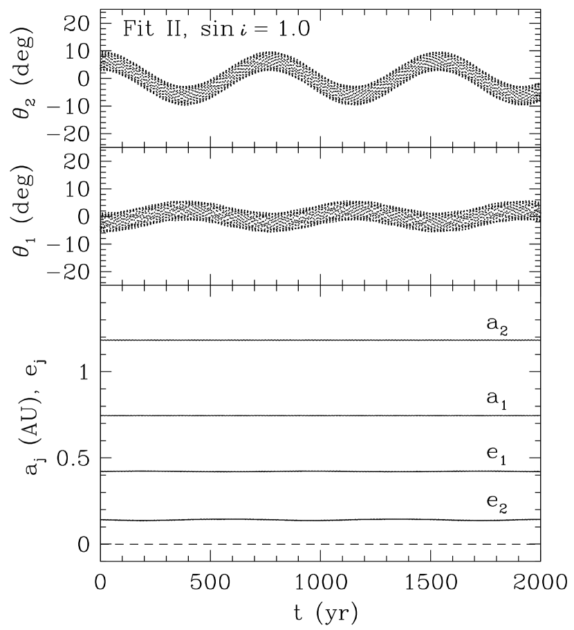
Figure 6: Evolution of the semimajor axes, $a_{1}$ and $a_{2}$, eccentricities, $e_{1}$ and $e_{2}$, and 2:1 mean-motion resonance variables, $\theta_{1}=\lambda_{1}-2\lambda_{2}+\varpi_{1}$ and $\theta_{2}=\lambda_{1}-2\lambda_{2}+\varpi_{2}$, for fit II with $\sin i=1$. The semiamplitude $\Delta\theta_{1}\approx 6^{\circ}$ and $\Delta\theta_{2}\approx 10^{\circ}$.

Mayor et al. (2004) have published 142 radial velocity measurements obtained between 1999 and 2003 in graphical form only. We have extracted their data from Figure 6 of Mayor et al. (2004) with an accuracy of about $0.5\,$d in the times of observation and an accuracy of about $0.07{\rm\,m\,s}^{-1}$ in the velocities and their internal uncertainties. The uncertainty of $0.5\,$d in the extracted time of observation can translate into a velocity uncertainty of as much as $2{\rm\,m\,s}^{-1}$ in the steepest parts of the radial velocity curve (where the radial velocity can change by as much as $4{\rm\,m\,s}^{-1}$ per day), but the square of even this maximum ($2{\rm\,m\,s}^{-1}$) is much smaller than the sum of the squares of the extracted internal uncertainty ($\gtrsim 4{\rm\,m\,s}^{-1}$) and the estimated stellar jitter ($4.2{\rm\,m\,s}^{-1}$). As another check of the quality of this extracted CORALIE data set, we have performed a double-Keplerian fit of the extracted data, with the extracted internal uncertainties as the measurement errors in the calculation of the reduced chi-square statistic $\chi_{\nu}^{2}$. The resulting best fit has RMS $=6.99{\rm\,m\,s}^{-1}$, which is only slightly larger than the RMS ($=6.8{\rm\,m\,s}^{-1}$) of the Mayor et al. best fit, and the orbital parameters agree with those found by Mayor et al. and reproduced in Table 1 to better than $\pm 2$ in the last digit. This confirms that the extracted data set is comparable in quality to the actual data set.

In the analysis below, we use the combined data set containing 165 velocity measurements and spanning $6.1{\rm\,yr}$, and we adopt the quadrature sum of the internal uncertainty and the estimated stellar jitter as the measurement error of each data point in the calculation of $\chi_{\nu}^{2}$.

3 DOUBLE-KEPLERIAN FITS

As we mention in §1, the mutual gravitational interaction of the planets is not expected to affect the radial velocity of HD 82943 significantly over the $6.1$-year time span (or about 5 outer planet orbits) of the available observations. Thus we fit the radial velocity $V_{r}$ of the star with the reflex motion due to two orbiting planetary companions on independent Keplerian orbits:

$$V_{r}=K_{1}\left[\cos(\omega_{1}+f_{1})+e_{1}\cos\omega_{1}\right]+K_{2}\left[\cos(\omega_{2}+f_{2})+e_{2}\cos\omega_{2}\right]+V,$$ (4)

where $V$ is the line-of-sight velocity of the center of mass of the whole planetary system relative to the solar system barycenter, $K_{j}$ is the amplitude of the velocity induced by the $j$th planet, and $e_{j}$, $\omega_{j}$ and $f_{j}$ are, respectively, the eccentricity, argument of periapse, and true anomaly of the $j$th planet’s orbit (see, e.g., Lee & Peale 2003b). The zero points of the velocities measured by different telescopes are different, and $V$ is a parameter for each telescope (denoted as $V_{K}$ and $V_{C}$ for the Keck and CORALIE data, respectively). Since the true anomaly $f_{j}$ depends on $e_{j}$, the orbital period $P_{j}$, and the mean anomaly ${\cal M}_{j}$ at a given epoch (which we choose to be the epoch of the first CORALIE measurement, JD 2451185.1), there are five parameters, $P_{j}$, $K_{j}$, $e_{j}$, $\omega_{j}$, and ${\cal M}_{j}$, for each Keplerian orbit. Thus there are a total of 12 parameters. The fact that the orbital parameters obtained from double-Keplerian fits should be interpreted as Jacobi (and not astrocentric) coordinates does not change the fitting function in equation (4) but changes the conversion from $K_{j}$ and $P_{j}$ to the planetary masses $m_{j}$ and orbital semimajor axes $a_{j}$:

$$K_{j}=\left(2\pi G\over P_{j}\right)^{1/3}{m_{j}\sin i_{j}\over{m^{\prime}_{j}}^{2/3}}{1\over\sqrt{1-e_{j}^{2}}},$$ (5)

$$P_{j}=2\pi[a_{j}^{3}/(Gm^{\prime}_{j})]^{1/2},$$ (6)

where ${m^{\prime}_{j}}=\sum_{k=0}^{j}m_{k}$ (Lee & Peale, 2003b). All of the orbital fits presented here are obtained using the Levenberg-Marquardt algorithm (Press et al., 1992) to minimize $\chi_{\nu}^{2}$. The Levenberg-Marquardt algorithm is effective at converging on a local minimum for given initial values of the parameters.

We begin by using the parameter values listed in Table 1 as the initial guess and allowing all 12 parameters to be varied in the fitting. The resulting fit I is listed in Table 3 and compared to the radial velocity data in Figure 1. We also show the residuals of the radial velocity data from fit I in the top panel of Figure 4. Fit I has $\chi_{\nu}^{2}=1.87$ for 12 adjustable parameters (or $1.84$ if we rescale $\chi_{\nu}^{2}$ to 10 adjustable parameters for comparison with the 10 parameter fits below) and RMS $=7.88{\rm\,m\,s}^{-1}$. However, fit I is dynamically unstable if the orbits are assumed to be coplanar. We perform a series of direct numerical orbit integrations of fit I similar to that described in §1 to test the stability of the Mayor et al. (2004) best-fit solution (i.e., with $\sin i=1$, $0.9$, $\ldots$, $0.5$ and four starting epochs equally spaced between JD 2451185.1 and JD 2452777.7). Figure 2 shows the evolution of the semimajor axes, $a_{1}$ and $a_{2}$, and eccentricities, $e_{1}$ and $e_{2}$, for the integration with $\sin i=1$ and starting epoch JD 2451185.1, which becomes unstable after $\sim 3200{\rm\,yr}$. All of the integrations of fit I become unstable in time ranging from $\sim 60$ to $3200{\rm\,yr}$.

We then explore fits in which one or two of the parameters are fixed at values different from those of fit I and the other parameters are varied. These experiments indicate that $e_{2}$ and $\omega_{2}$ are the least constrained parameters, as there are fits with $e_{2}$ and $\omega_{2}$ fixed at values very different from those of fit I that have $\chi_{\nu}^{2}$ (after taking into account the difference in the number of adjustable parameters) and RMS only slightly different from those of fit I. Therefore, we decide to examine systematically best-fit double-Keplerian models with fixed values of $e_{2}$ and $\omega_{2}$. We start at $e_{2}=0.22$ and $\omega_{2}=290^{\circ}$ (which are close to the values for fit I), using the parameters of fit I as the initial guess for the other 10 parameters. Then for each point on a grid of resolution $0.01$ in $e_{2}$ and $5^{\circ}$ in $\omega_{2}$, we search for the best fit with fixed $e_{2}$ and $\omega_{2}$, using the best-fit parameters already determined for an adjacent grid point as the initial guess.

Figure 3 shows the contours of $\chi_{\nu}^{2}$, RMS, $e_{1}$, $\omega_{1}$, and the planetary mass ratio $m_{1}/m_{2}$ for the best-fit double-Keplerian models with fixed values of $e_{2}$ and $\omega_{2}$. Fit I at $e_{2}=0.219$ and $\omega_{2}=284^{\circ}$ is the only minimum in $\chi_{\nu}^{2}$, with $\chi_{\nu}^{2}=1.84$ for 10 adjustable parameters. However, the minimum is relatively shallow, with $\chi_{\nu}^{2}\lesssim 2.0$ in a region that includes the entire region with $e_{2}\lesssim 0.2$ and extends to $e_{2}\approx 0.38$ near $\omega_{2}=130^{\circ}$ and $280^{\circ}$. The contours of RMS are similar to those of $\chi_{\nu}^{2}$. The RMS minimum (where RMS $=7.87{\rm\,m\,s}^{-1}$) at $e_{2}=0.22$ and $\omega_{2}=275^{\circ}$ is only slightly offset from the $\chi_{\nu}^{2}$ minimum, and the region with $\chi_{\nu}^{2}\lesssim 2.0$ also has RMS $\lesssim 8.2{\rm\,m\,s}^{-1}$. The contours of $e_{1}$, $\omega_{1}$, and $m_{1}/m_{2}$ show that these parameters are indeed well constrained, with $e_{1}$ within $\pm 0.05$ of $0.39$, $\omega_{1}$ within $\pm 15^{\circ}$ of $120^{\circ}$, and $m_{1}/m_{2}$ within $\pm 0.2$ of $1.0$ for the fits with $\chi_{\nu}^{2}\lesssim 2.0$.

In Figure 3a we mark the positions of three fits II–IV (as well as fit I) whose dynamical properties are discussed in detail in §4. Their orbital parameters are listed in Table 3, and the residuals of the radial velocity data from these fits are shown in the lower three panels of Figure 4. We can infer from the parameters listed in Table 3 that the fits II–IV have nearly identical $a_{1}$($\approx 0.747{\rm\,AU}$), $a_{2}$($\approx 1.18{\rm\,AU}$), and $m_{2}\sin i$($\approx 1.71\,M_{J}$, where $M_{J}$ is the mass of Jupiter) while $m_{1}\sin i$ ranges from $1.58\,M_{J}$ for fit II to $1.78\,M_{J}$ for fit IV. Figure 4 demonstrates visually that these fits with $\chi_{\nu}^{2}$ only slightly higher than the minimum are comparable in the quality of fit to the fit I with the minimum $\chi_{\nu}^{2}$.

4 DYNAMICAL ANALYSIS

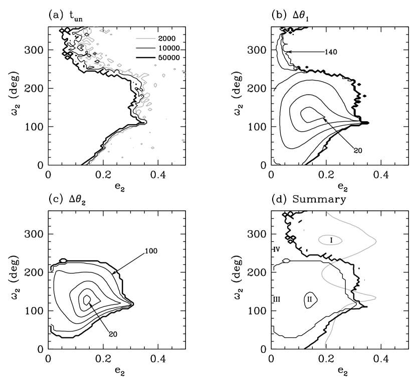
Figure 5: Dynamical properties of the best-fit double-Keplerian models shown in Fig. 3 for $\sin i=1$. (a) Contours of the time $t_{\rm un}$ (in units of yr) at which a model becomes unstable. (b) Contours of the semiamplitude $\Delta\theta_{1}$ in steps of $20^{\circ}$. (c) Contours of the semiamplitude $\Delta\theta_{2}$ in steps of $20^{\circ}$ from $20^{\circ}$ to $100^{\circ}$. The thick solid contour is the boundary for the libration of $\theta_{2}$. (d) Positions of fits I–IV in the $e_{2}$-$\omega_{2}$ plane. The gray contours are $\chi_{\nu}^{2}=1.85$ and $2.0$. The thick solid contour is $t_{\rm un}=5\times 10^{4}{\rm\,yr}$. The thin solid contours are $\Delta\theta_{2}=30^{\circ}$ and the boundary for the libration of $\theta_{2}$. Only fits with $\Delta\theta_{1}\lesssim 140^{\circ}$ are stable for at least $5\times 10^{4}{\rm\,yr}$. Fit I at the minimum of $\chi_{\nu}^{2}$ is unstable. Fit II is the stable fit with the smallest libration amplitudes of both $\theta_{1}$ and $\theta_{2}$. Fit III is a stable fit with large amplitude librations of both $\theta_{1}$ and $\theta_{2}$. Fit IV is a stable fit with only $\theta_{1}$ librating.

We begin with some general remarks on the dynamical properties of the best-fit double-Keplerian models with fixed $e_{2}$ and $\omega_{2}$ that can be inferred from the contour plots in Figure 3. There is a wide variety of stable 2:1 resonance configurations with both $\theta_{1}$ and $\theta_{2}$ librating (see, e.g., Lee 2004). For $m_{1}/m_{2}\sim 1$, there are (1) the sequence of resonance configurations that can be reached by the differential migration of planets with constant masses and initially coplanar and nearly circular orbits, (2) the sequence with large $e_{2}$ and asymmetric librations of both $\theta_{1}$ and $\theta_{2}$ far from either $0^{\circ}$ or $180^{\circ}$, and (3) the sequence with $\theta_{1}$ librating about $180^{\circ}$ and $\theta_{2}$ librating about $0^{\circ}$. Their loci in the $e_{1}$-$e_{2}$ plane are shown in Figures 5, 11, and 14, respectively, of Lee (2004). The good fits in Figure 3 have $e_{1}\approx 0.39\pm 0.05$ and $e_{2}\lesssim 0.38$, which are far from the loci of the sequences 2 and 3. Thus the good fits in Figure 3 cannot be small-libration-amplitude configurations in the sequences 2 and 3. Figure 3d shows that the fits with $\omega_{2}\approx 120^{\circ}$ also have $\omega_{1}\approx 120^{\circ}$. These fits with $\theta_{\rm SAR}=\varpi_{1}-\varpi_{2}\approx 0^{\circ}$ currently also have $e_{1}\gtrsim 0.40$ and $m_{1}/m_{2}\lesssim 1.0$, and we can infer from Figure 5 of Lee (2004) for the sequence 1 that the fits with $e_{2}\approx 0.14$ and $\omega_{2}\approx 120^{\circ}$ could be in a symmetric configuration with both $\theta_{1}$ and $\theta_{2}$ (and hence $\theta_{\rm SAR}$) librating about $0^{\circ}$ with small amplitudes. However, direct numerical orbit integrations are needed to determine whether the fits with $e_{2}\approx 0.14$ and $\omega_{2}\approx 120^{\circ}$ are in fact in such a resonance configuration. Finally, Figure 5 of Lee (2004) also shows that there are configurations in the sequence 1 with asymmetric librations of $\theta_{1}$ and $\theta_{2}$ in the region $e_{1}\approx 0.39\pm 0.05$ and $e_{2}\lesssim 0.38$ if $m_{1}/m_{2}\gtrsim 0.95$, and we cannot rule out the possibility of asymmetric librations for the fits in Figure 3 with $m_{1}/m_{2}\gtrsim 0.95$ without direct numerical orbit integrations.

In order to use dynamical stability to narrow the range of reasonable fits and to determine the actual dynamical properties of the stable fits, we perform direct numerical orbit integrations of all of the best-fit double-Keplerian models with fixed $e_{2}$ and $\omega_{2}$ shown in Figure 3. We use the symplectic integrator SyMBA (Duncan et al., 1998) and assume that the orbital parameters obtained from the fits are in Jacobi coordinates (Lee & Peale 2003b; see also Lissauer & Rivera 2001). Double-Keplerian fits do not yield the inclinations of the orbits from the plane of the sky. We assume that the orbits are coplanar and consider two cases: $\sin i=1$ and $0.5$. We perform integrations for only one starting epoch, JD 2451185.1, since for each fit we already examine neighboring fits with slightly different orbital parameters. The maximum time interval of each integration is $5\times 10^{4}\,$yr. An integration is stopped and the model is considered to have become unstable, if (1) the distance of a planet from the star is less than $0.075{\rm\,AU}$ or greater than $3.0{\rm\,AU}$ or (2) there is an encounter between the planets closer than the sum of their physical radii for an assumed mean density of $1{\rm\,g\,cm}^{-3}$. For these planets with orbital periods of about 220 and 440 days, $a_{1}\approx 0.75{\rm\,AU}$, $a_{2}\approx 1.2{\rm\,AU}$, and their physical radii are about 0.011 and 0.0066 of their Hill radii for a mean density of $1{\rm\,g\,cm}^{-3}$.

In Figure 5 we present the results of the direct numerical orbit integrations for $\sin i=1$. Figure 5a shows the contours of the time, $t_{\rm un}$, at which a model becomes unstable, and Figure 5b shows the contours of the semiamplitude $\Delta\theta_{1}$. All of the fits that are stable for at least $5\times 10^{4}{\rm\,yr}$ have $\theta_{1}$ librating about $0^{\circ}$ with $\Delta\theta_{1}\lesssim 140^{\circ}$. Figure 5c shows the contours of the semiamplitude $\Delta\theta_{2}$, with the thick solid contour indicating the boundary for the libration of $\theta_{2}$ about $0^{\circ}$. None of the stable fits shows asymmetric libration of $\theta_{1}$ or $\theta_{2}$. Since the region with $\theta_{2}$ librating is smaller than that with $\theta_{1}$ librating, there are stable good fits with only $\theta_{1}$ librating about $0^{\circ}$, in addition to stable good fits with both $\theta_{1}$ and $\theta_{2}$ librating about $0^{\circ}$. The fits with $e_{2}\approx 0.14$ and $\omega_{2}\approx 130^{\circ}$ have small amplitude librations of both $\theta_{1}$ and $\theta_{2}$ about $0^{\circ}$, in good agreement with the estimate of $e_{2}\approx 0.14$ and $\omega_{2}\approx 120^{\circ}$ above.

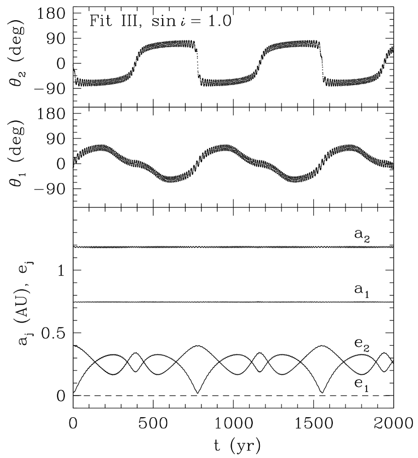
Figure 7: Same as Fig. 6, but for fit III with $\sin i=1$. The semiamplitude $\Delta\theta_{1}\approx 68^{\circ}$ and $\Delta\theta_{2}\approx 82^{\circ}$.

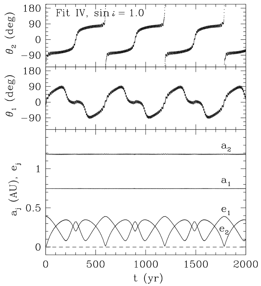
Figure 8: Same as Fig. 6, but for fit IV with $\sin i=1$. The semiamplitude $\Delta\theta_{1}\approx 94^{\circ}$, and $\theta_{2}$ circulates.

The contour for $\Delta\theta_{2}=30^{\circ}$ and the boundary for the libration of $\theta_{2}$ are compared to the contour for $t_{\rm un}=5\times 10^{4}{\rm\,yr}$ and the contours for $\chi_{\nu}^{2}=1.85$ and $2.0$ in Figure 5d, where the positions of the fits I–IV are also indicated. We can see from Figure 5d that the fit I with the minimum $\chi_{\nu}^{2}$, which is unstable (Fig. 2), is in fact far from the stability boundary. Fit II at $e_{2}=0.14$ and $\omega_{2}=130^{\circ}$ is the fit with the smallest libration amplitudes of both $\theta_{1}$ and $\theta_{2}$. The evolution of $a_{j}$, $e_{j}$, and $\theta_{j}$ for $2000{\rm\,yr}$ for fit II with $\sin i=1$ is shown in Figure 6. The semiamplitude $\Delta\theta_{1}\approx 6^{\circ}$ and $\Delta\theta_{2}\approx 10^{\circ}$, and the small amplitudes ensure that both $a_{j}$ and $e_{j}$ have little variation. Fit III at $e_{2}=0.02$ and $\omega_{2}=130^{\circ}$ is an example of a stable fit with large amplitude librations of both $\theta_{1}$ and $\theta_{2}$. The semiamplitude $\Delta\theta_{1}\approx 68^{\circ}$ and $\Delta\theta_{2}\approx 82^{\circ}$, the eccentricity $e_{1}$ varies between $0.16$ and $0.40$ and $e_{2}$ between $0.02$ and $0.33$ (see Fig. 7). Finally, fit IV at $e_{2}=0.02$ and $\omega_{2}=260^{\circ}$ is an example of a stable fit with only $\theta_{1}$ librating. Figure 8 shows that $\theta_{2}$ circulates through $\pm 180^{\circ}$ when $e_{2}$ is very small. The semiamplitude $\Delta\theta_{1}\approx 94^{\circ}$, the eccentricity $e_{1}$ varies between $0.08$ and $0.39$ and $e_{2}$ between $0.008$ and $0.35$.

While the fits with small amplitude librations of both $\theta_{1}$ and $\theta_{2}$ should be indefinitely stable, stability for $5\times 10^{4}{\rm\,yr}$ does not in general guarantee stability on much longer timescales. Indeed the changes in the contours for $t_{\rm un}=2000$, $10^{4}$, and $5\times 10^{4}{\rm\,yr}$ in Figure 5a indicate that the region of fits with only $\theta_{1}$ librating is likely to be significantly smaller for stability on much longer timescales. We confirm that the fit IV with only $\theta_{1}$ librating, as well as fits II and III, are stable for at least $10^{8}{\rm\,yr}$ by performing direct integrations of these fits for $10^{8}{\rm\,yr}$. However, direct integrations of the fits at $e_{2}=0.02$ and $\omega_{2}=360^{\circ}$ and $310^{\circ}$ show that these fits become unstable after $6.0\times 10^{6}$ and $3.4\times 10^{7}{\rm\,yr}$, respectively.

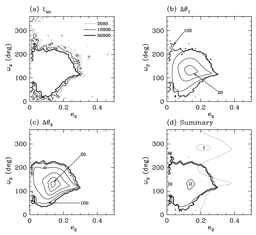
Figure 9: Same as Fig. 5, but for $\sin i=0.5$. Only fits with both $\theta_{1}$ and $\theta_{2}$ librating are stable, and fits I and IV are unstable.

In Figure 9 we present the results of the direct numerical orbit integrations for $\sin i=0.5$. The range of fits that are stable for at least $5\times 10^{4}{\rm\,yr}$ is significantly smaller than that for $\sin i=1$ (compare Figs. 5a and 9a). There are small regions where the fits have only $\theta_{1}$ librating about $0^{\circ}$ and they are stable for $5\times 10^{4}{\rm\,yr}$ (see Fig. 9d), but the changes in the contours for $t_{\rm un}=2000$, $10^{4}$, and $5\times 10^{4}{\rm\,yr}$ in Figure 9a indicate that these fits are unlikely to be stable on much longer timescales. Thus, for $\sin i=0.5$, only fits with both $\theta_{1}$ and $\theta_{2}$ librating about $0^{\circ}$ are stable. The unstable fit I is again far from the stability boundary. Fit IV, which is stable for at least $10^{8}{\rm\,yr}$ for $\sin i=1$, is unstable for $\sin i=0.5$. Direct integrations for $10^{8}{\rm\,yr}$ show that fits II and III with $\sin i=0.5$ are stable for at least $10^{8}{\rm\,yr}$. We can see from Figures 5b and 9b and Figures 5c and 9c that there are only small changes in the contours of the semiamplitudes $\Delta\theta_{1}$ and $\Delta\theta_{2}$ for the fits that are stable for both $\sin i=0.5$ and $1$. This means that the changes in $\Delta\theta_{1}$ and $\Delta\theta_{2}$ with $\sin i$ are small for most of the fits that are stable for both $\sin i=0.5$ and $1$. In particular, fit II is also the fit with the smallest libration amplitudes of both $\theta_{1}$ and $\theta_{2}$ for $\sin i=0.5$. Figure 10 (compared to Fig. 6) shows that the libration period is shorter due to the larger planetary masses but that $\Delta\theta_{1}$ and $\Delta\theta_{2}$ are within $1^{\circ}$ of the values for $\sin i=1$. We do not show the time evolution of $\theta_{1}$ and $\theta_{2}$ for fit III with $\sin i=0.5$, but $\Delta\theta_{1}$ and $\Delta\theta_{2}$ are again within $1^{\circ}$ of the values for $\sin i=1$.

5 DISCUSSION AND CONCLUSIONS

We have analyzed the HD 82943 planetary system by examining the best-fit double-Keplerian model to the radial velocity data as a function of the poorly constrained eccentricity and argument of periapse of the outer planet’s orbit. We have not found any good fits that are non-resonant and dynamically stable (if the orbits are assumed to be coplanar), and the two planets in the HD 82943 system are almost certainly in 2:1 mean-motion resonance. The fit I with the minimum $\chi_{\nu}^{2}$ is unstable, but there is a wide range of fits outside the minimum with $\chi_{\nu}^{2}$ only slightly higher than the minimum. If the unknown $\sin i\approx 1$, there are stable good fits with both of the mean-motion resonance variables, $\theta_{1}=\lambda_{1}-2\lambda_{2}+\varpi_{1}$ and $\theta_{2}=\lambda_{1}-2\lambda_{2}+\varpi_{2}$, librating about $0^{\circ}$ (e.g., fits II and III), as well as stable good fits with only $\theta_{1}$ librating about $0^{\circ}$ (e.g., fit IV). If $\sin i\approx 0.5$, only good fits with both $\theta_{1}$ and $\theta_{2}$ librating about $0^{\circ}$ (e.g., fits II and III) are stable. Fit II is the fit with the smallest libration semiamplitudes of both $\theta_{1}$ and $\theta_{2}$, with $\Delta\theta_{1}\approx 6^{\circ}$ and $\Delta\theta_{2}\approx 10^{\circ}$.

Our analysis differs from that of Ferraz-Mello et al. (2005) in having the additional Keck data, in using $\chi_{\nu}^{2}$ instead of RMS as the primary measure of the goodness of fit, and in examining systematically the dynamical properties of all of the fits found. Although Ferraz-Mello et al. (2005) showed $e_{j}$ and $\omega_{j}$ of many fits with RMS within $\approx 0.2{\rm\,m\,s}^{-1}$ of the minimum RMS, they discussed in detail the dynamical properties of only two fits — their solutions A and B — with RMS within $0.06{\rm\,m\,s}^{-1}$ of the minimum. Their solutions A and B have $\omega_{1}\approx 120^{\circ}$ and $\omega_{2}\gtrsim 200^{\circ}$ and hence large amplitude librations of both $\theta_{1}$ and $\theta_{2}$. Because the fit to the CORALIE data with the minimum RMS (which is near the minimum $\chi_{\nu}^{2}$ fit of Mayor et al. 2004 at $e_{2}=0.18$ and $\omega_{2}=237^{\circ}$; see Table 1) is close to the stability boundary in the $e_{2}$-$\omega_{2}$ plane, Ferraz-Mello et al. (2005) were able to find stable fits with RMS within $0.06{\rm\,m\,s}^{-1}$ of the minimum. For the combined data set, the fit with the minimum RMS at $e_{2}=0.22$ and $\omega_{2}=275^{\circ}$ is far from the stability boundary, and none of our fits with RMS within $0.06{\rm\,m\,s}^{-1}$ of the minimum are stable (see Figs. 3b, 5a, and 9a). However, by examining systematically the $\chi_{\nu}^{2}$, RMS, and dynamical properties of all of our fits, we have found fits like fit IV (which has stable, large amplitude libration of only $\theta_{1}$ if $\sin i\approx 1.0$), fit III (which has large amplitude librations of both $\theta_{1}$ and $\theta_{2}$) and, in particular, fit II (which has small amplitude librations of both $\theta_{1}$ and $\theta_{2}$), all with RMS within $0.13{\rm\,m\,s}^{-1}$ of the minimum and $\chi_{\nu}^{2}$ within $0.08$ of the minimum. The stable and unstable regions in the $e_{2}\cos\omega_{2}$-$e_{2}\sin\omega_{2}$ plane shown in Figures 4 and 8 of Ferraz-Mello et al. (2005) are qualitatively similar to those in our Figures 5a and 9a in the $e_{2}$-$\omega_{2}$ plane, but it should be noted that their figures show simulations of their solution B (for the CORALIE data) with $e_{2}$ and $\omega_{2}$ changed, while our figures show simulations of the fits (to the combined data set) that minimize $\chi_{\nu}^{2}$ for the given $e_{2}$ and $\omega_{2}$.

The relatively large values of $\chi_{\nu}^{2}$ ($\geq 1.84$) and RMS ($\geq 7.87{\rm\,m\,s}^{-1}$) of the fits presented in this paper suggest that the double-Keplerian model may not fully explain the radial velocity data of HD 82943. Also hinting at the same possibility is the increase in the RMS of the best fit from $6.99{\rm\,m\,s}^{-1}$ (for the extracted CORALIE data alone) to $7.88{\rm\,m\,s}^{-1}$ with the inclusion of the Keck data, which fill in some gaps in the CORALIE data and increase the time span of observations. However, the RMS and $\chi_{\nu}^{2}$ values are by themselves not very strong evidence, because our estimate ($4.2{\rm\,m\,s}^{-1}$) for the radial velocity jitter has an uncertainty of $\sim 50\%$ and the jitter can be $\sim 6{\rm\,m\,s}^{-1}$. On the other hand, there appears to be systematic deviations of the radial velocity data from the double-Keplerian fits. Figure 4 shows that the data within about $\pm 200$ days of JD 2452600 are higher than the fits and that the data near JD 2453181 are lower than the fits. The fact that $\sim 40\%$ of the Keck measurements fall in these two regions result in the aforementioned increase in the RMS of the best fit from $6.99{\rm\,m\,s}^{-1}$ for the CORALIE data alone to $7.88{\rm\,m\,s}^{-1}$ for the combined data set. But it is important to note that the Keck and CORALIE data are consistent with each other where they overlap and that they are both higher than the fits in the region around JD 2452600. One possible explanation for the deviations is that they are due to the mutual gravitational interaction of the planets. However, unlike the GJ 876 system where the resonance-induced apsidal precession rate $d\varpi_{j}/dt$ is $-41^{\circ}{\rm\,yr}^{-1}$ on average and the precession has been seen for more than one full period (Laughlin et al., 2005), the average apsidal precession rates of, e.g., fits II and III are only $-0\fdg 51\,(\sin i)^{-1}{\rm\,yr}^{-1}$ and $-0\fdg 71\,(\sin i)^{-1}{\rm\,yr}^{-1}$, respectively, and the orbits have precessed a negligible $3$–$4\,(\sin i)^{-1}$ degrees over the $6.1{\rm\,yr}$ time span of the available observations. On the other hand, there are small variations in the orbital elements on shorter timescales due to the planetary interaction that could produce deviations from the double-Keplerian model. Alternatively, the deviations could be due to the presence of additional planet(s). Continued observations of HD 82943 combined with dynamical fits should allow us to distinguish these possibilities.

Table 1: Orbital Parameters of the HD 82943 Planets from Mayor et al. (2004)

Parameter		Inner		Outer
$P$ (days)		219.4		435.1
$K$ (${\rm m}\,{\rm s}^{-1}$)		61.5		45.8
$e$		0.38		0.18
$\omega$ (deg)		124		237
${\cal M}$ (deg)		357		246

Note. — The parameters are the orbital period $P$, the velocity amplitude $K$, the orbital eccentricity $e$, the argument of periapse $\omega$, and the mean anomaly ${\cal M}$ at the epoch JD 2451185.1.

Table 2: Measured Velocities for HD 82943 from Keck

JD		Radial Velocity		Uncertainty
($-$2450000)		(${\rm m}\,{\rm s}^{-1}$)		(${\rm m}\,{\rm s}^{-1}$)
2006.913		43.39		3.2
2219.121		23.58		2.7
2236.126		30.29		2.7
2243.130		38.46		2.6
2307.839		$-$46.33		3.2
2332.983		$-$11.26		3.4
2333.956		$-$12.25		3.3
2334.873		$-$0.65		3.0
2362.972		25.02		3.3
2389.944		47.81		3.1
2445.739		55.26		3.0
2573.147		$-$48.70		2.9
2575.140		$-$46.26		2.6
2576.144		$-$50.28		3.1
2601.066		$-$22.60		3.1
2602.073		$-$15.76		2.9
2652.001		19.60		3.1
2988.109		$-$89.93		2.8
3073.929		$-$4.31		3.1
3153.754		0.41		2.8
3180.745		$-$62.93		2.7
3181.742		$-$54.04		3.1
3397.908		$-$99.57		2.8

Table 3: Orbital Parameters of the HD 82943 Planets

Parameter		Inner		Outer
Fit I [$\chi_{\nu}^{2}=1.87$, $\chi_{\nu}^{2}(10)=1.84$, RMS $=7.88{\rm\,m\,s}^{-1}$]
$P$ (days)		219.3		441.2
$K$ (${\rm m}\,{\rm s}^{-1}$)		66.0		43.6
$e$		0.359		0.219
$\omega$ (deg)		127		284
${\cal M}$ (deg)		353		207
$m\sin i$ ($M_{J}$)		2.01		1.75
$V_{K}$ (${\rm m}\,{\rm s}^{-1}$)	-6.3
$V_{C}$ (${\rm m}\,{\rm s}^{-1}$)	8143.9
Fit II ($\chi_{\nu}^{2}=1.92$, RMS $=8.00{\rm\,m\,s}^{-1}$)
$P$ (days)		219.6		436.7
$K$ (${\rm m}\,{\rm s}^{-1}$)		53.5		42.0
$e$		0.422		0.14
$\omega$ (deg)		122		130
${\cal M}$ (deg)		357		352
$m\sin i$ ($M_{J}$)		1.58		1.71
$V_{K}$ (${\rm m}\,{\rm s}^{-1}$)	-6.9
$V_{C}$ (${\rm m}\,{\rm s}^{-1}$)	8142.7
Fit III ($\chi_{\nu}^{2}=1.91$, RMS $=7.99{\rm\,m\,s}^{-1}$)
$P$ (days)		219.5		438.8
$K$ (${\rm m}\,{\rm s}^{-1}$)		58.1		41.7
$e$		0.398		0.02
$\omega$ (deg)		120		130
${\cal M}$ (deg)		357		356
$m\sin i$ ($M_{J}$)		1.74		1.71
$V_{K}$ (${\rm m}\,{\rm s}^{-1}$)	-6.3
$V_{C}$ (${\rm m}\,{\rm s}^{-1}$)	8143.2
Fit IV ($\chi_{\nu}^{2}=1.90$, RMS $=7.97{\rm\,m\,s}^{-1}$)
$P$ (days)		219.5		439.2
$K$ (${\rm m}\,{\rm s}^{-1}$)		59.3		41.7
$e$		0.391		0.02
$\omega$ (deg)		121		260
${\cal M}$ (deg)		356		227
$m\sin i$ ($M_{J}$)		1.78		1.72
$V_{K}$ (${\rm m}\,{\rm s}^{-1}$)	-6.2
$V_{C}$ (${\rm m}\,{\rm s}^{-1}$)	8143.3

Note. — Fits II–IV are 10 parameter fits with fixed $e$ and $\omega$ of the outer planet’s orbit. Fit I is a 12 parameter fit, and its $\chi_{\nu}^{2}$ is shown both at its true value and at the value rescaled to 10 adjustable parameters for comparison with the 10 parameter fits. In addition to the parameters $P$, $K$, $e$, $\omega$, and ${\cal M}$, the minimum planetary mass, $m\sin i$, and the zero-point velocities, $V_{K}$ and $V_{C}$, of the Keck and CORALIE data, respectively, are listed.

Figure 1: Radial velocity curve of the double-Keplerian fit I (with the minimum $\chi_{\nu}^{2}$) compared to the Keck (filled circles) and CORALIE (open triangles) data for HD 82943. The error bars show the quadrature sum of the internal uncertainties and estimated stellar jitter ($4.2{\rm\,m\,s}^{-1}$).

Figure 2: Evolution of the semimajor axes, $a_{1}$ and $a_{2}$, and eccentricities, $e_{1}$ and $e_{2}$, for fit I with $\sin i=1$ and starting epoch JD 2451185.1. The system becomes unstable after $\sim 3200{\rm\,yr}$.

Figure 3: Parameters of the best-fit double-Keplerian models for HD 82943 for fixed values of the eccentricity, $e_{2}$, and argument of periapse, $\omega_{2}$, of the outer planet’s orbit. (a) Contours of $\chi_{\nu}^{2}$ in steps of 0.05 from 1.85 to 2.0 and then in steps of 0.25 to 3.0. The positions of fits I–IV are marked. (b) Contours of the RMS of the residuals (in units of ${\rm m}\,{\rm s}^{-1}$) in steps of 0.1 from 7.9 to 8.2 and then in steps of 0.6 to 10. (c) Contours of the eccentricity, $e_{1}$, of the inner orbit in steps of 0.02 from 0.3 to 0.5. (d) Contours of the argument of periapse, $\omega_{1}$, of the inner orbit in steps of $10^{\circ}$ from $80^{\circ}$ to $150^{\circ}$. (e) Contours of the planetary mass ratio $m_{1}/m_{2}$ in steps of 0.1 from 0.7 to 1.2. The ratio $m_{1}/m_{2}$ is nearly independent of $\sin i$, as long as $\sin i$ is not very small and $m_{1},m_{2}\ll m_{0}$.

Figure 4: Residual velocities from fits I–IV of the Keck (filled circles) and CORALIE (open triangles) data for HD 82943. The error bars show the quadrature sum of the internal uncertainties and estimated stellar jitter ($4.2{\rm\,m\,s}^{-1}$).

Figure 10: Same as Fig. 6, but for fit II with $\sin i=0.5$. The semiamplitudes $\Delta\theta_{1}$ and $\Delta\theta_{2}$ are within $1^{\circ}$ of the values for $\sin i=1$.

References

- Beaugé et al. (2003) Beaugé, C., Ferraz-Mello, S., & Michtchenko, T. A. 2003, ApJ, 593, 1124
- Cumming et al. (1999) Cumming, A., Marcy, G. W., & Butler, R. P. 1999, ApJ, 526, 890
- Duncan et al. (1998) Duncan, M. J., Levison, H. F., & Lee, M. H. 1998, AJ, 116, 2067
- Ferraz-Mello et al. (2003) Ferraz-Mello, S., Beaugé, C., & Michtchenko, T. A. 2003, Celest. Mech. Dyn. Astron., 87, 99
- Ferraz-Mello et al. (2005) Ferraz-Mello, S., Michtchenko, T. A., & Beaugé, C. 2005, ApJ, 621, 473
- Fischer & Valenti (2005) Fischer, D. A., & Valenti, J. 2005, ApJ, 622, 1102
- Kley et al. (2005) Kley, W., Lee, M. H., Murray, N., & Peale, S. J. 2005, A&A, 437, 727
- Kley et al. (2004) Kley, W., Peitz, J., & Bryden, G. 2004, A&A, 414, 735
- Laughlin et al. (2005) Laughlin, G., Butler, R. P., Fischer, D. A., Marcy, G. W., Vogt, S. S., & Wolf, A. S. 2005, ApJ, 622, 1182
- Laughlin & Chambers (2001) Laughlin, G., & Chambers, J. E. 2001, ApJ, 551, L109
- Laws et al. (2003) Laws, C., Gonzalez, G., Walker, K. M., Tyagi, S., Dodsworth, J., Snider, K., & Suntzeff, N. B. 2003, AJ, 125, 2664
- Lee (2004) Lee, M. H. 2004, ApJ, 611, 517
- Lee & Peale (2002) Lee, M. H., & Peale, S. J. 2002, ApJ, 567, 596
- Lee & Peale (2003a) Lee, M. H., & Peale, S. J. 2003a, in Scientific Frontiers in Research on Extrasolar Planets, ed. D. Deming & S. Seager (San Francisco: ASP), 197
- Lee & Peale (2003b) Lee, M. H., & Peale, S. J. 2003b, ApJ, 592, 1201
- Lissauer & Rivera (2001) Lissauer, J. J., & Rivera, E. J. 2001, ApJ, 554, 1141
- Marcy et al. (2001) Marcy, G. W., Butler, R. P., Fischer, D., Vogt, S. S., Lissauer, J. J., & Rivera, E. J. 2001, ApJ, 556, 296
- Mayor et al. (2004) Mayor, M., Udry, S., Neaf, D., Pepe, F., Queloz, D., Santos, N. C., & Burnet, M. 2004, A&A, 415, 391
- Papaloizou (2003) Papaloizou, J. C. B. 2003, Celest. Mech. Dyn. Astron., 87, 53
- Press et al. (1992) Press, W. H., Teukolsky, S. A., Vetterling, W. T., & Flannery, B. P. 1992, Numerical Recipes in Fortran 77: The Art of Scientific Computing (Cambridge: Cambridge Univ. Press)
- Rivera & Lissauer (2001) Rivera, E. J., & Lissauer, J. J. 2001, ApJ, 558, 392
- Rivera et al. (2005) Rivera, E. J., Lissauer, J. J., Butler, R. P., Marcy, G. W., Vogt, S. S., Fischer, D. A., Brown, T. M., Laughlin, G., & Henry, G. W. 2005, ApJ, 634, 625
- Saar et al. (1998) Saar, S. H., Butler, R. P., & Marcy, G. W. 1998, ApJ, 498, L153
- Santos et al. (2000a) Santos, N. C., Israelian, G. & Mayor, M. 2000a, A&A, 363, 228
- Santos et al. (2000b) Santos, N. C., Mayor, M., Naef, D., Pepe, F., Queloz, D., Udry, S., & Blecha, A. 2000b, A&A, 361, 265
- Wright (2005) Wright, J. T. 2005, PASP, 117, 657