The Intra-Night Optical Variability of the bright BL Lac object S5 0716+714

Abstract

Aims. We address the topic of the Intra-Night Optical Variability of the BL Lac object S5 0716+714.

Methods. To this purpose a long term observational campaign was performed, from 1996 to 2003, which allowed the collection of a very large data set, containing 10,675 photometric measurements obtained in 102 nights.

Results. The source brightness varied in a range of about 2 mag, although the majority of observations were performed when it was in the range $13.0<R<13.75$. Variability time scales were estimated from the rates of magnitude variation, which were found to have a distribution function well fitted by an exponential law with a mean value of 0.027 mag/h, corresponding to an e-folding time scale of the flux $\tau_{F}=$ 37.6 h. The highest rates of magnitude variation were around 0.10–0.12 mag/h and lasted less than 2 h. These rates were observed only when the source had an $R$ magnitude $<$ 13.4, but this finding cannot be considered significant because of the low statistical occurrence. The distribution of $\tau_{F}$ has a well defined modal value at 19 h. Assuming the recent estimate of the beaming factor $\delta\sim$ 20, we derived a typical size of the emitting region of about 5$\times$10${}^{16}/(1+z)$ cm. The possibility to search for a possible correlation between the mean magnitude variation rate and the long term changes of the velocity of superluminal components in the jet is discussed.

1 Introduction

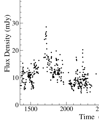
The radio source S5 0716+714  was identified with a bright and highly variable BL Lac object, characterized by a strong featureless optical continuum (Biermann et al. 1981). The failure in detecting a host galaxy both in HST direct imaging (Urry et al. 2000) and in high S/N spectra (Rector & Stocke 2001) suggests that its redshift $z$ should be greater than 0.52 (Sbarufatti et al. 2005; see also Schalinski et al. 1992 and Wagner et al. 1996). Variations on short time scales (a fraction of hour) have been detected in several occasions at frequencies ranging from radio to X-rays (Quirrenbach et al. 1991; Wagner et al. 1996; Gabuzda et al. 2000; Heidt & Wagner 1996; Nesci et al. 2002; Giommi et al. 1999; Villata et al. 2000; Wu et al. 2005). The recent history of the flux of S5 0716+714  in the $R$ (Cousins) band is plotted in Fig. 1, which spans the time interval from 1997 to 2003. The photometric points up to 2001 have been extracted from the data base by Raiteri et al. (2003), taking only one measurement per day, whereas points from 2002 to 2003 are new data obtained by our group (Nesci et al. 2005). The general structure of this curve shows that the mean flux of S5 0716+714  varies in the range 5-20 mJy with some flares in which it reaches and overwhelms 30 mJy. These flares are separated by time intervals variable from $\sim$ 1 to $\sim$ 3 years. In Fig. 1 there are four large flares having a typical duration of the order of 1–2 months from which it is possible to estimate a flaring duty cycle of about 5–10%.

Figure 1: The light curve in the $R$(Cousins) band of S5 0716+714  from February 1997 to March 2003. Vertical bars on the top mark the epochs of our INOV observations.

In this paper we focus our attention on the so called Intra-Night Optical Variability (INOV) or microvariability. Brightness changes of BL Lac objects, having amplitudes of about 10–20% and occurring on time scales as short as a fraction of an hour, were studied since the eighties by Miller and coworkers (Miller et al. 1989; Carini et al. 1991). This phenomenon was after detected in many sources of this class and it could be considered one of their characterizing properties. INOV in BL Lac objects and other blazars has been investigated by several authors, using either single or multi band photometry: among BL Lac objects showing such activity we recall AO 0235+164 (Romero et al. 2000), S4 0954+658 (Papadakis et al. 2004), BL Lacertae (Massaro et al. 1998; Nesci et al. 1998; Papadakis et al. 2003) whereas studies on samples of sources are those on LBL (Low energy peaked BL Lacs) objects (Heidt & Wagner 1996), EGRET blazars (Romero et al. 2002) and other BL Lac objects and radio-core dominated blazars (Sagar et al. 2004; Stalin et al. 2005). These works are generally based on data sets, for single sources, obtained in a not high number of nights and/or observations. Moreover, the analysis is mainly focused on the search for recurrence time scales detectable in the individual light curves.

A first detailed study of INOV in S5 0716+714  is that of Wagner et al. (1996), who investigated rapid variations in multifrequency (from radio to X-rays) campaigns and observed a quasi-periodic behaviour with a typical recurrence time of about two days and a high correlation between the optical and radio flux changes. The possibility of an harmonic component in the optical flux of S5 0716+714  was after confirmed by Heidt & Wagner (1996), who did not detect a similar effect on the other BL Lacs of their sample. Sagar et al. (1999) reported INOV multiband observations covering 4 weeks in 1994 and found only three major events of rapid variability in which the highest magnitude variation rate was around 0.03 mag/h. Villata et al. (2000) reported the results of a WEBT (Whole Earth Blazar Telescope) campaign on S5 0716+714  from 16 to 22 February 1999 in which a relevant INOV was observed every night with magnitude variation rates up to $\sim$ 0.1 mag/h.

A well established definition of INOV properties for a given source (or for a class of sources) can be obtained only from the analysis of a relatively large number of observations, possibly performed in different brightness states.

The definition of time scale for non-periodic phenomena is not univocal and can depend on the type of variation: in this work we consider a time scale based on the magnitude variation rates.

We worked extensively on S5 0716+714, bright enough to obtain good photometric data with small aperture telescopes and short exposure times. Our INOV observational campaign of S5 0716+714  started in 1996 and since November 1998 we undertook a more intense data acquisition concluded in spring 2003. In this paper we report a large set of observational data, containing 10,675 photometric points, obtained in 102 nights, which is up to now the largest database of INOV for any BL Lac object. Our statistical analysis will give new informations on the distribution of the variability time scales and other properties of this source.

2 Observations and Data Reduction

Most of our photometric observations of S5 0716+714  were performed with a 32 cm f/4.5 Newtonian reflector located near Greve in Chianti (Tuscany) with a CCD camera, manufactured by DTA, mounting a back-illuminated SITe SIA502A chip. A few observations were made with the 50 cm telescope of the Astronomical Station of Vallinfreda (Rome) and the 70 cm telescope, formerly at Monte Porzio (Rome), both equipped with CCD cameras. Standard $B$, $V$ (Johnson), $R$ (Cousins) and $I$ (Cousins) filters were used. Exposure times depended upon the brightness of the source and varied between 3 and 5 minutes to have a typical noise level on the comparison stars of 0.01 mag or less.

Differential photometry with respect to three or four comparison stars in the same field of view of S5 0716+714  was performed using the apphot task in IRAF . The same circular aperture, with a radius of 5 arcsec was used for the photometry of S5 0716+714  and the comparison stars. These were the A, B, C, D stars of the reference sequence given by Ghisellini et al. (1997), corresponding to stars 2, 3, 5, 6 of the sequence by Villata et al. (1998). Our large number of images gave the possibility to calculate (for our bandpasses and detector response) their magnitude intercalibration with a high accuracy and consequently we modified the original $B$, $V$, $R$ values to minimize the measured uncertainties, while for the $I$ band those given by Ghisellini et al. (1997) were unchanged. The adopted values are listed in Table 1.

Table 1: $B$, $V$, $R$, $I$ magnitudes of reference stars used in our analysis.

Star	$B$	$V$	$R$	$I$
A, 2	12.03	11.51	11.20	10.92
B, 3	13.06	12.48	12.10	11.79
C, 5	14.17	13.58	13.20	12.85
D, 6	14.25	13.66	13.28	12.97

We took as best estimate of the errors of the S5 0716+714  magnitudes the rms value of the reference stars’ values combined with the statistical error of the pixel counts. These resulted generally of the order of 0.01 mag. We verified a posteriori that the typical scatter of the data of S5 0716+714  around a smoothed 4-6 point running average curve was fully compatible with this error estimate. In a small number of cases we found some data showing large discrepancies with respect to the nearest points or having uncertainties much larger than the others. We believed that such large differences are of instrumental origin, due to a possible occurrence of hot/cold pixels or a noise fluctuation. We preferred to cancel these data from the light curves rather than to correct their values: their number was generally quite small and light curves were unaffected by the removal. Moreover, some light curves were taken in unstable and not photometric nights and the data scatter with respect to the running averages was higher. Noisy segments or entire curves were discarded from the data set to avoid the inclusion of poor data and possible spurious effects.

Figure 2: Histogram of the mean $R$ magnitude in the nights of INOV observations.

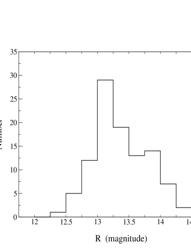
Table The Intra-Night Optical Variability of the bright BL Lac object S5 0716+714 reports the log of all good quality observations considered in the present paper: for each night we give the date of observation (column 1), the abridged JD (column 2), the UT start time (column 3), the observation duration (column 4), the number of frames (column 5), the filter used (column 6), the mean magnitude of the source in the used filter (column 7), the rms deviation of the magnitude difference between two reference stars (column 8), the telescope (column 9: G=Greve, M=Monte Porzio, V=Vallinfreda) and the number of time intervals used in the evaluation of the magnitude variation rates (column 10). The entire photometric data set including measured magnitudes of S5 0716+714, not corrected for the interstellar reddening, and errors is given in Table A1, described in the Appendix and available in electronic form at CDS.

An histogram of the mean magnitude of S5 0716+714  during our intranight observations is given in Fig. 2. The source brightness varied in a range of about 2 mag, but the majority of observations were performed when it was in the range $13.0<R<13.75$.

As the host galaxy is undetected (an upper limit of $R>20$ mag is given by Urry et al. 2000) no correction needs to be applied to our photometric values.

Figure 3: Some examples of INOV of S5 0716+714  observed at different epochs from 2000 to 2003. The solid lines through the data show the linear best fit used to evaluate $|\Delta m/\Delta t|$ in each selected interval. Date of observations are 02-01-2000 (top left), 12-01-2000 (top right), 26-02-2001 (middle left), 03-11-2001 (middle right), 22-04-2002 (bottom left), 23-03-2003 (bottom right).

3 Light curves and variability time scale

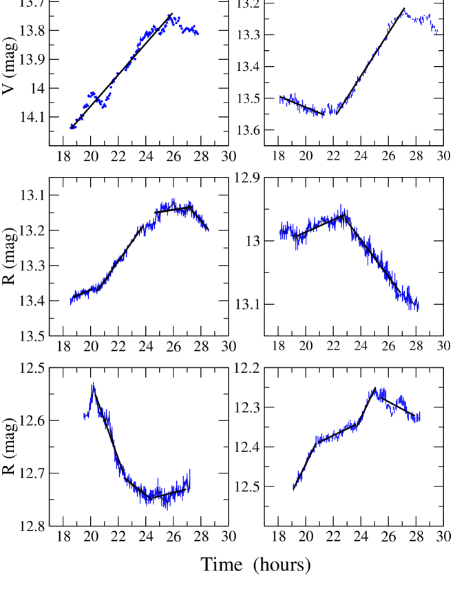
As mentioned in the Introduction, INOV is a frequent characteristic of the optical emission of S5 0716+714. We detected significant brightness changes in a large fraction of nights: only in 9 nights (marked with an asterisk in Table The Intra-Night Optical Variability of the bright BL Lac object S5 0716+714) the source remained stable during the observation time window. Some light curves showing examples of relevant INOV of S5 0716+714  are plotted in the panels of Fig. 3: in these cases the variation amplitudes were larger than 0.1 mag and overwhelmed 0.3 mag in some of them. In some occasions light curves show oscillations of about 0.05–0.1 mag with a typical duration of a few hours. From Table The Intra-Night Optical Variability of the bright BL Lac object S5 0716+714 we see that the rms value of the difference between two reference stars was generally within one or two hundredths of magnitude confirming the reality of these oscillations. Some examples will be described in Sect. 4.

The time scale of flux variations can be defined as

$$\tau_{F}=\frac{1}{1+z}\,\,\frac{F_{\nu}}{|dF_{\nu}/dt|}$$ (1)

which, when it can be considered constant, corresponds to the e-folding time scale. The factor $1+z$ takes into account cosmological effects. This definition of variability time scale is similar, but not coincident, with that used by Romero et al. (2002), who adopted the flux variation $\Delta F$ measured in the night instead of $F$. With their definition, time scales resulted comparable or shorter than the durations of the observations, while with our definition the result is less related to the length of time windows. The value of $\tau_{F}$ can be directly computed from the magnitude light curves $m(t)$, because its variation rate corresponds to the log-derivative of $F$. In fact, from the classic Pogson’s formula of astronomical photometry, we have:

$$\bigg{|}\frac{dm}{dt}\bigg{|}=2.5\leavevmode\nobreak\ \bigg{|}\frac{d}{dt}Log\leavevmode\nobreak\ F_{\nu}\bigg{|}=\frac{1.086}{\tau_{F}}$$ (2)

Figure 4: The solid histogram is the number distribution of the decreasing values of $\Delta m/\Delta t$ while the dashed one is that for the increasing values.

To derive the values of $\tau_{F}$ we divided each light curve into a few monotonic intervals. For each interval we fitted the light curve with a straight line and accepted the best fitting slope value as our estimate of $\Delta m/\Delta t$. Obviously, the selection of these segments is a delicate task that cannot be performed by means of a simple algorithm because of the large variety of light curve shapes. We were aware that subjective selection criteria, which can introduce some bias, are unavoidable and in order to reduce this possibility we adopted the following procedure:

• the number of selected intervals per night must be as small as possible;

• the selected time intervals must be long enough to contain a sufficient number ($>10$, but typically $>20$, i.e. two hours) of data points;

• time intervals cannot overlap;

• segments must be compatible with a constant magnitude variation rate, which was verified looking for trends in the residuals with respect to a linear best fit;

• magnitude oscillations of small amplitude and short duration superposed to a longer trend, like those described below in Sect. 4, were not considered to evaluate $\Delta m/\Delta t$.

In all cases a linear fit was fully adequate to describe the selected segments of the light curves with no systematic structure left in the residuals.

The number of time intervals taken into account for each night is indicated in Table The Intra-Night Optical Variability of the bright BL Lac object S5 0716+714. The total number of intervals is 204 with a mean number per night equal to 2. Only in 8 nights, over a total number of 102, light curves were found particularly structured to take into account 4 or 5 intervals. Note, however, that 5 of these nights are in the last month of our campaign (from the end of February to that of March 2003), that could correspond to a period in which S5 0716+714  exhibited variations faster than usual. Finally we recall that only in 9 nights the source was stable (formal fit slope less than 0.002 mag/h).

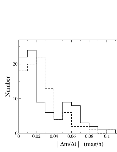
We checked if there were differences in the distributions of the rising and decreasing values of $\Delta m/\Delta t$. A Kolmogorov-Smirnov test gives no difference at the 98.3% confidence level: the histogram is reported in Fig. 4. Therefore the statistical analysis of the distribution of $\Delta m/\Delta t$ (and corresponding $\tau_{F}$) is performed on their absolute values.

Figure 5: The solid histogram is the frequency distribution of all the variation rates $|\Delta m/\Delta t|$ (in mag/h) in all the used filters. Dotted line is the exponential law best fit. The dashed histogram is that obtained using just the highest rate ($|\Delta m/\Delta t|_{max}$) measured in each night.

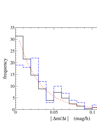
Fig. 5 shows the frequency histogram (i.e. number of data in each bin divided by the bin width) of all measured $|\Delta m/\Delta t|$ that can be very well represented by the exponential distribution (dashed line):

$$f(|\dot{m}|)=K\leavevmode\nobreak\ exp(-|\dot{m}|/\langle|\dot{m}|\rangle)$$ (3)

with $\langle|\dot{m}|\rangle$ = 0.027 mag/h and the best fit value of the normalisation constant $K=$ 36.5, very close to the theorical value $1/\langle|\dot{m}|\rangle$.

Figure 6: Frequency histogram of the variability time scales $\tau_{F}$. Dashed line is the best fit of the theorical distribution given by Eq. (5).

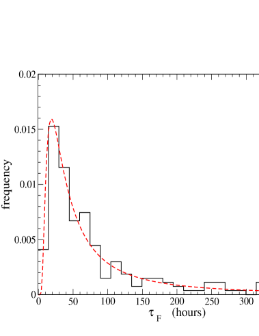
The statistical distribution of $\dot{m}$ (the time derivative of $m$, in our case $|\Delta m/\Delta t|$) and of $\tau_{F}$ satisfy the relation:

$$f(\dot{m})=\frac{1}{\tau_{F}^{2}}f(\tau_{F})$$ (4)

Appling this relation, the distribution of $\tau_{F}$ is

$$f(\tau_{F})=\frac{K^{\prime}}{\tau_{F}^{2}}\leavevmode\nobreak\ exp(-\tau_{F}^{*}/\tau_{F})$$ (5)

with $\tau_{F}^{*}=1.086/\langle|\dot{m}|\rangle$. Fig. 6 shows the resulting histogram for $\tau_{F}$ and the best fit of the distribution given in Eq. (5); in particular, $\tau_{F}^{*}$ is equal to 37.6 h, in a very good agreement with the expected value.

In computing the parameters of this distribution we did not include very small $|\dot{m}|$ values which would give $\tau_{F}$ longer than 350 h. We point out that the mean value of variable $\tau_{F}$ cannot be computed from the first moment of Eq. (5) because, once multiplied by $\tau_{F}$, the integral does not converge. So a direct calculation of $\langle\tau_{F}\rangle$ from the values is not statistically correct: indeed a very small value of $|\dot{m}|$ (a flat light curve segment) corresponds to a very high $\tau_{F}$ that pushes the mean towards an infinit value. A much better statistically defined parameter useful to describe this distribution is the mode $\tau_{Fm}$. It can be calculated from the maximum of Eq. (5), which occurs at $\tau_{Fm}=\tau_{F}^{*}/2$, corresponding to 18.8 h.

Figure 7: Plot of $|\Delta m/\Delta t|$ vs $\Delta t$, the magnitude variation rates against the duration of the corresponding time intervals.

In Fig. 5 we plotted also the histogram (dashed line) of $|\Delta m/\Delta t|_{max}$ obtained considering the highest variation rates measured in each night: the content of the bins above 0.03 mag/h is slightly changed, whereas the frequencies in two lower bins are much smaller. This histogram is useful to evaluate the probability of how large a magnitude variation rate can be in the typical observation window of a night (say eight-nine hours), even when the time interval in which the variation occurs is shorter. We see that rates $\sim$ 0.03 mag/h are the most frequently measured.

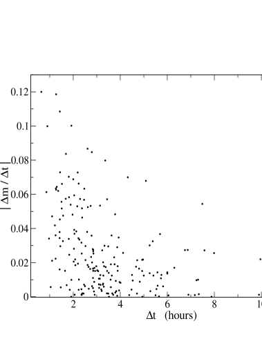
We also studied whether there is a relation between $|\Delta m/\Delta t|$ and the duration of the time intervals $\Delta t$. Fig. 7 shows the plot of these two variables: we can see that most intervals have durations in the range 2–4 h and that in only few cases durations longer than 9 h were detected. Note that in three of the latter occasions we measured low rates and only in one case it was close to 0.05 mag/h. Variation rates greater than 0.1 mag/h were measured only over time intervals shorter than 2 h, indicating that such high rates do not remain stable for long time intervals. On the other side, note that rates smaller than 0.02 mag/h were found for intervals of any duration confirming that the probability to observe the source brightness steady is much higher than that to find a large INOV, as expected from the exponential distribution in Fig. 5. We can also conclude that magnitude variation rates higher than 0.1 mag/h are a rare phenomenon having a probability lower than a few percent.

Figure 8: The variation rates (in mag/h) plotted against the mean $R$ magnitude of the source. Note that the rates above 0.085 mag/h were found only when S5 0716+714  was brighter than $R=13.4$, while lower rates were found in any brightness states.

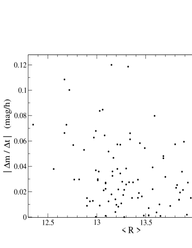
We also searched for a possible relation between INOV and the mean brightness state of S5 0716+714. The plot in Fig. 8 shows the distribution of largest values of $|\Delta m/\Delta t|$ measured in each light curve against the mean value of $R$ in that night. When the used filter was different we derived approximate $R$ value applying the mean colour indices given by Raiteri et al. (2003), which were found generally stable. The points corresponding to rates with $|\Delta m/\Delta t|<$ 0.08 mag/h appears to be rather uniformly distributed, whereas a possible deviation from uniformity can be seen in the upper region, corresponding to the highest rates. These rates, in fact, were measured only when S5 0716+714  was brighter than $R\simeq$ 13.4, an indication that a faster INOV is more likely when the source is brighter: the statistical significance of this finding, however, is limited by the small number of measures. We remark, anyway, that these high rates were not found within a short observation window, but are distributed from 2000 to 2003.

Finally we briefly comment on the possibility that the magnitude variation rates can be different for different photometric bands. Actually we have 3 nights in B band, 6 in I, 15 in V and 78 in R (see Table The Intra-Night Optical Variability of the bright BL Lac object S5 0716+714: the number of nights with filters different from R is very limited, and the variation of the color index of the source in the historical data base (Raiteri et al. 2003) is rather small, and without a clear correlation with the source luminosity, so we do not expect a detectable difference in the distribution of the $\tau_{F}$ values. A formal Kolmogorov-Smirnov test between the $\tau_{F}$ distribution derived from the R-band data and that derived from the BVI ones gives no indication of differences.

4 Micro-oscillations

In the previous section we mentioned that in several occasions the INOV of S5 0716+714  was characterized by oscillations of very small amplitude, typically $<$ 0.10 mag. Two examples of such a behaviour can be seen in Fig. 3 and precisely in the light curves of 2000 January 2 (top left panel) and 2003 March 23 (bottom right panel). Recently Wu et al. (2005) reported the observation of a similar oscillation with an amplitude of 0.05 mag, a duration of about 5 hours and without a detectable colour change. They discuss also about the possible origin of this type of INOV and conclude that it could be due to a geometric modulation as expected in the helical jet model by Camenzind & Krockenberger (1992).

Small amplitude oscillations are occasionally superposed onto variations characterised by longer trends. Fig. 9 shows the light curve observed on 2000 January 2 (see also Fig. 3, top left panel) when a couple of consecutive micro-oscillations were detected in the interval from 18.60 to 25.85 UT. To make these oscillations more evident we fitted the interval where they are present with a straight line and subtracted the interpolated magnitudes from the original data set. The curve of the magnitude differences with respect to the linear best fit is plotted in the lower panel: the resulting oscillation amplitude is $\sim$ 0.05 mag and the duration is about 3 h. For comparison we plotted in both panels the differences of the magnitudes of two reference stars: they remain much more stable than the source, not only in the magnitude variation shown in the upper panel, but also with respect to the differences in the lower panel. Note also the regularity of these changes that cannot be confused with a spurious effect due to noisy observations. We conclude that this particular INOV can be originated neither by variations of the atmospheric extinction nor by other instrumental effects and that it must be considered genuine.

Figure 9: The light curve in the $V$ band observed on 2000 January 2. Upper panel shows photometric data of S5 0716+714  (filled circles) and the magnitude difference of two reference stars (open triangles), shifted by an arbitrary offset; the dashed line is the linear best fit of a brightening segment. Lower panel shows the difference of S5 0716+714  magnitude with respect to the best fit line to show the micro-oscillations: in this case the amplitude is $\sim$ 0.05 mag and the duration of a cycle is $\sim$ 3 h.

Figure 10: Micro-oscillation of the brightness of S5 0716+714  observed on 2003 February 25. Triangles are the difference between the magnitude of two reference stars with an arbitrary offset. Note the noise increase in the last two hours in both light curves.

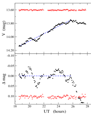
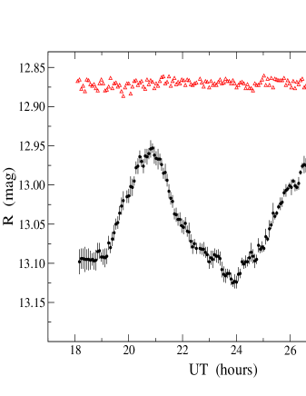
Fig. 10 shows another micro-oscillation detected on 2003 February 25. In this case the amplitude was of $\sim$ 0.1 mag with a duration of $\sim$ 6.5 h. Because of its relatively long duration it was segmented into three intervals to evaluate the magnitude variation rate. Note in the last portion of the curves of both S5 0716+714  and reference stars the effect of a noise increase likely due to the incoming twilight.

Note also that the light curve of 2000 January 12 (see the upper right panel in Fig. 3) could be considered as a micro oscillation with respect to the mean brightening trend covering all the night. In this case it would have an amplitude of $\sim$ 0.1 mag and a duration of $\sim$ 11 h.

The oscillating behaviour was already noticed in other occasions (Wagner et al. 1996; Heidt & Wagner 1996; Villata et al. 2000). All these examples indicate that the micro-oscillating behaviour is not particularly rare but, at the same time, it does not have a stable pattern. A quantitative estimate of their frequency, however, is rather difficult, because their detection is limited by the duration of the observing window. The examples presented above suggest the possibility that longer variations can have typically larger amplitudes than the short ones. The confirmation of this hypothesis on a statistical ground requires a collection of INOV light curves even greater than ours.

5 Discussion

The observational results described in this paper are useful to extend the present knowledge about INOV of BL Lac objects. In an about six year long campaign we obtained a large collection of data on S5 0716+714, not available before for a single source, useful to develop a statistical study of the main INOV properties. We give in Table A1 (see Appendix) the whole data set, including all 10,675 photometric measurements. They can be used for further investigations and for a comparison with other data on the same and other sources.

Our statistical analysis was essentially based on the evaluation of magnitude variation rates $|\Delta m/\Delta t|$ over several time intervals, selected using rather uniform criteria to minimize possible biases. We found that the resulting distribution is fully compatible with an exponential one having a mean $\langle|\Delta m/\Delta t|\rangle=$ 0.027 mag/h, corresponding to a flux variation time scale of 37.6 h. This finding implies that the probability to observe a magnitude variation rate higher than 0.2 mag/h is smaller than 10^-3, and therefore one would require more than 500 nights of observations like ours to detect an episode having such a high rate.

The interpretation of the variability of blazars is not a simple problem because it involves the description of rapidly changing processes characterized by several physical quantities, whose mean values and statistical distributions are poorly known. The fact that we found an exponential distribution for $|\Delta m/\Delta t|$ without any evidence of a typical time scale suggests that the INOV is essentially a stochastic process. A possibility already considered in some papers is that of a turbulent jet. A model in which relativistic electrons emit synchrotron radiation in a turbulent magnetic field was described by Marscher et al. (1992): the resulting light curves show trends and oscillations like those described in the previous sections. This agreement is, however, only qualitative and a larger observational effort should be performed to achieve a more detailed description of the turbulence parameters. For instance, the discovery of a relation between the amplitude and the duration of small oscillations on a robust statistical ground can help to model the turbulence.

Another investigation can concern the possible long term variations of INOV parameters. Nesci et al. (2005) recently presented the historic light curve of S5 0716+714  that shows a well apparent brightening trend since about 25 years. A study of the apparent ejection velocities of superluminal blobs in the jet $\beta_{ej}$ (Bach et al. 2005) showed that it decreased from $\sim$ 15 to $\sim$ 5 in the period from 1986 to 1997. Both effects are consistent with a scenario of a precessing jet having a stable Lorentz factor $\Gamma\simeq 12$ but approaching the line of sight from an angle of about 5^∘ to 0^∘.5. The corresponding Doppler factor $\delta=1/\Gamma(1-\beta\,cos\theta)$ ($\Gamma$ is the bulk Lorentz factor, and $\theta$ the angle between the jet direction and the line of sight) increased from $\sim$ 13 to $\sim$ 25.

We can use this independent estimate of $\delta$ to constrain the size of the emitting region responsible for INOV. Considering the mode $\tau_{Fm}$ of the distribution in Fig. 6 as a typical (short) timescale and assuming $\delta\simeq 20$ (Nesci et al. 2005), we can derive an upper limit to the characteristic size of the emitting region in the comoving frame $r^{\prime}\simeq c\,\delta\,\tau_{Fm}/(1+z)\simeq 5\times 10^{16}/(1+z)$ cm, a value which agrees well with those usually adopted in modelling BL Lac jets.

The distribution of the magnitude variation rates is useful to detect a change in the jet orientation. Indeed, if synchrotron emission is originated in a relativistic jet, the observed flux is related to the one emitted in the comoving frame $F^{\prime}$ (assumed practically steady) by the relativistic boosting:

$$F(t)=(\delta(t))^{k}F^{\prime}$$ (6)

where $k=3+\alpha$ ($\alpha$ is the spectral index). After converting the flux in magnitude and deriving with respect to the time:

$$|\dot{m}|=1.086\leavevmode\nobreak\ k\,|\dot{\delta}/\delta|$$ (7)

If the variation of $\delta$ is due only to the change of $\theta$, we obtain

$$|\dot{\delta}/\delta|=\beta_{app}|\dot{\theta}|$$ (8)

and

$$|\dot{m}|=1.086\,k\,\beta_{app}|\dot{\theta}|$$ (9)

where $\beta_{app}=(\beta\leavevmode\nobreak\ sin\theta)/(1-\beta\leavevmode\nobreak\ cos\theta)=-d(1-\beta\leavevmode\nobreak\ cos\theta)^{-1}/d\theta$ is the apparent velocity of superluminal components along the jet. This relation suggests that in the case of a regular variation of $\theta$ (precessing jet) it is possible to expect a positive correlation between $\langle|\dot{m}|\rangle$ and $\beta_{app}$. Under this respect, it will be important to continue to study this blazar: we expect that an increase of $\theta$, after the very low value reached in the past years, would imply an increasing $\beta_{app}$ and consequently a larger $\langle|\dot{m}|\rangle$ (see also Nesci et al. 2005).

This consideration supports the importance of a multifrequency approach to distinguish geometrical from physical effects affecting the emission properties of BL Lac objects. Massaro & Mantovani (2004) pointed out how the study of both optical long-term variability and VLBI imaging can be useful for the understanding of geometrical and structural changes of the synchrotron radiation in jets of BL Lacs. Now we suggest the possibility that the mean properties of INOV, say for instance $\langle|\dot{m}|\rangle$ or $\tau_{Fm}$, may also change on such long time scales and could be related to the kinematics of the jet derived from VLBI imaging. This kind of work requires the acquisition and storage of a large amount of INOV observations for a sample of BL Lac objects, covering time intervals of several decades. Such a great observational effort can be performed only with the collaboration of several groups, possibly working with automatic/robotic small aperture telescopes, and with the creation of homogeneous and well organized databases.

[x]lrrrrccccc Log of INOV observations of S5 0716+714. (Total number of frames: 10,675).
Date JD Start time Duration Frames Filter Mean mag. $\Delta$Comp. rms Tel. Intervals
($-2449000$) UT (hh:mm) (hours)
continued.
Date JD Start time Duration Frames Filter Mean mag. $\Delta$Comp. rms Tel. Intervals
($-2449000$) UT (hh:mm) (hours)
1996/11/12 1400 20:59 6.87 88 B 14.31 0.016 V 2
1997/03/03 * 1511 20:00 6.58 49 B 14.81 0.016 V 1
1997/03/12 1520 19:11 6.17 34 B 14.76 0.008 V 2
1998/11/07 2125 18:29 9.38 101 R 13.80 0.008 G 2
1998/12/17 2165 18:13 10.53 108 R 14.13 0.008 G 2
1998/12/18 2166 16:49 5.73 69 R 14.23 0.006 G 1
1999/01/05 2184 17:22 8.62 96 R 14.05 0.009 G 1
1999/03/13 2251 18:51 8.93 113 I 13.29 0.007 G 2
1999/03/14 2252 18:59 3.63 85 I 12.91 0.007 M 1
1999/11/26 2509 17:55 11.34 133 V 14.57 0.018 G 1
1999/11/27 2510 19:01 10.01 128 V 14.72 0.013 G 3
1999/12/07 2520 18:02 6.72 71 V 14.53 0.009 G 1
2000/01/02 2546 18:34 9.20 126 V 13.91 0.007 G 1
2000/01/12 2556 18:09 11.40 138 V 13.41 0.007 G 2
2000/01/15 2559 18:20 9.36 121 V 13.99 0.008 G 2
2000/01/16 2560 19:46 9.12 103 V 14.06 0.013 G 1
2000/01/19 2563 18:34 10.92 89 V 14.31 0.014 G 2
2000/01/25 2569 18:18 10.74 150 V 14.01 0.009 G 4
2000/02/20 * 2595 20:51 6.00 67 V 14.41 0.011 M 1
2000/03/05 2609 19:22 8.37 101 V 14.69 0.010 G 2
2000/03/06 2610 18:39 6.04 71 V 14.41 0.008 G 1
2000/03/20 2624 18:24 9.37 109 R 14.15 0.011 G 3
2000/03/21 2625 19:03 9.05 106 R 14.13 0.008 G 2
2000/04/21 2656 19:31 4.61 62 V 14.17 0.013 G 1
2000/04/25 2660 19:43 7.12 86 V 14.30 0.008 G 2
2000/10/23 2841 18:05 8.88 130 R 12.77 0.007 G 2
2000/10/27 2845 18:40 7.72 111 V 13.09 0.009 G 2
2000/10/28 2846 18:22 7.01 97 R 12.67 0.023 G 3
2000/12/04 2883 16:50 9.61 117 R 12.87 0.009 G 3
2000/12/18 2897 17:38 9.36 83 R 13.85 0.011 G 2
2000/12/31 * 2910 18:35 6.58 92 R 13.53 0.013 G 1
2001/01/14 2924 17:35 10.64 146 R 13.07 0.012 G 3
2001/01/21 * 2931 19:27 7.70 98 R 13.28 0.009 G 1
2001/02/10 2951 18:44 9.72 127 R 13.19 0.009 G 2
2001/02/11 2952 18:33 9.01 129 R 13.30 0.006 G 3
2001/02/14 2955 17:45 10.55 146 R 13.42 0.006 G 3
2001/02/20 2961 17:45 6.11 75 R 13.30 0.007 G 2
2001/02/26 2967 18:33 10.00 146 R 13.24 0.009 G 4
2001/04/14 * 3014 19:24 5.38 74 R 13.65 0.009 G 1
2001/04/17 3017 20:47 6.46 84 R 13.53 0.006 G 1
2001/04/28 3028 19:57 7.26 94 R 13.21 0.008 G 2
2001/08/19 * 3141 20:08 5.58 67 R 12.99 0.015 G 1
2001/08/23 3145 21:12 6.12 82 R 12.99 0.008 G 2
2001/08/24 * 3146 20:31 7.06 99 R 13.09 0.010 G 1
2001/08/26 3148 21:07 6.39 92 R 13.15 0.006 G 3
2001/09/03 3156 19:31 5.50 78 R 13.25 0.010 G 1
2001/09/06 3159 19:58 7.10 95 R 13.12 0.007 G 1
2001/09/10 3163 19:08 8.53 122 R 13.26 0.009 G 3
2001/09/12 3165 20:22 7.52 108 R 13.09 0.011 G 3
2001/10/11 3194 19:47 7.69 108 R 12.82 0.007 G 2
2001/10/12 3195 17:59 10.49 141 I 12.44 0.009 G 2
2001/10/18 3201 18:32 3.88 54 R 12.90 0.006 G 1
2001/11/03 3217 18:07 10.04 139 R 13.01 0.007 G 2
2001/11/04 3218 21:58 5.85 69 B 13.90 0.007 G 2
2001/11/04 3218 17:25 3.95 45 R 13.22 0.008 G 1
2001/11/16 * 3230 17:23 9.81 97 R 13.48 0.011 G 1
2002/01/25 3300 17:18 6.91 93 R 13.68 0.011 G 2
2002/02/01 3307 19:04 8.19 114 R 13.70 0.005 G 2
2002/02/02 3308 17:48 11.07 156 R 13.68 0.006 G 2
2002/02/03 3309 18:13 9.46 129 R 13.84 0.007 G 2
2002/03/10 3344 19:41 8.81 116 R 13.12 0.012 G 2
2002/03/11 3345 18:45 9.83 125 R 13.28 0.006 G 2
2002/03/13 3347 18:59 8.77 125 R 13.09 0.006 G 3
2002/03/15 3349 19:12 9.23 130 R 13.22 0.006 G 2
2002/03/20 3354 18:43 9.32 126 R 13.27 0.008 G 2
2002/03/25 3359 18:51 9.36 123 R 13.08 0.010 G 4
2002/03/27 3361 18:42 6.38 89 B 13.91 0.013 G 2
2002/04/01 3366 18:50 8.89 122 R 13.21 0.008 G 2
2002/04/21 3386 19:04 7.27 95 R 12.72 0.014 G 3
2002/04/22 3387 19:30 7.68 107 R 12.69 0.011 G 3
2002/05/01 3396 19:24 7.31 101 R 12.90 0.007 G 2
2002/05/13 3408 19:35 5.24 63 R 12.93 0.013 G 1
2002/05/14 3409 19:46 7.07 95 R 13.37 0.007 G 1
2002/05/17 3412 21:07 5.67 82 R 13.16 0.009 G 1
2002/05/29 3424 20:43 5.78 71 R 13.84 0.010 G 1
2002/05/30 3425 20:26 5.92 65 R 13.61 0.012 G 1
2002/09/30 3548 18:34 5.52 70 R 13.82 0.008 G 2
2002/10/28 3576 19:19 8.37 110 R 13.93 0.008 G 2
2002/10/29 3577 18:02 9.66 129 R 13.96 0.008 G 2
2002/11/04 3583 18:57 10.01 133 R 13.46 0.006 G 2
2002/11/06 3585 18:49 5.77 67 R 13.24 0.006 G 2
2002/12/29 3638 17:30 12.25 175 R 13.17 0.011 V 1
2003/01/18 * 3658 18:20 9.60 132 R 13.53 0.009 G 1
2003/01/26 3666 18:43 10.95 153 R 13.20 0.007 G 1
2003/01/27 3667 19:22 7.30 99 R 13.15 0.009 G 1
2003/02/01 3672 18:18 10.95 156 R 13.19 0.009 G 1
2003/02/02 3673 19:16 7.97 104 R 13.16 0.006 G 3
2003/02/09 3680 18:26 10.72 138 R 13.36 0.005 G 2
2003/02/10 3681 18:24 11.03 149 R 13.33 0.006 G 3
2003/02/11 3682 18:53 10.16 144 R 13.57 0.007 G 1
2003/02/17 3688 17:56 5.19 69 R 13.44 0.013 G 2
2003/02/18 3689 18:20 10.92 159 R 13.34 0.009 G 3
2003/02/24 3695 19:31 5.91 85 R 13.34 0.004 G 4
2003/02/25 3696 18:10 11.00 157 R 13.03 0.006 G 5
2003/02/26 3697 18:16 10.58 75 I 12.57 0.007 G 2
2003/03/04 3703 19:02 9.40 138 R 13.06 0.005 G 2
2003/03/07 3706 20:19 7.46 49 R 13.32 0.024 G 1
2003/03/13 3712 18:20 10.30 81 I 12.24 0.012 G 3
2003/03/18 3717 18:59 8.63 115 R 12.97 0.012 G 5
2003/03/19 3718 18:25 10.43 64 I 12.51 0.008 G 1
2003/03/22 3721 19:34 8.68 123 R 12.56 0.009 G 4
2003/03/23 3722 19:06 9.16 125 R 12.35 0.008 G 4

Appendix A

In this Appendix we report a brief description of the entire data set of our photometric observations to study the INOV of S5 0716+714. All the data are organised in Table A1 as follows: each light curve is reported in three columns containing UT time in hours (column 1), source magnitude (column 2) and its error (column 3), derived as written in Sect. 2; each light curve is identified by a title with the date (DD-MM-YYYY) and the used filter.