The luminosity-weighted or ‘marked’ correlation function

Abstract

We present measurements of the redshift-space luminosity-weighted or ‘marked’ correlation function in the SDSS. These are compared with a model in which the luminosity function and luminosity dependence of clustering are the same as that observed, and in which the form of the luminosity-weighted correlation function is entirely a consequence of the fact that massive halos populate dense regions. We do this by using mock catalogs which are constrained to reproduce the observed luminosity function and the luminosity dependence of clustering, as well as by using the language of the redshift-space halo-model. These analyses show that marked correlations may show a signal on large scales even if there are no large-scale physical effects—the statistical correlation between halos and their environment will produce a measureable signal. Our model is in good agreement with the measurements, indicating that the halo mass function in dense regions is top-heavy; the correlation between halo mass and large scale environment is the primary driver for correlations between galaxy properties and environment; and the luminosity of the central galaxy in a halo is different from (in general, brighter than) that of the other objects in the halo. Thus our measurement provides strong evidence for the accuracy of these three standard assumptions of galaxy formation models. These assumptions also form the basis of current halo-model based interpretations of galaxy clustering.

When the same galaxies are weighted by their $u-$, $g-$, or $r-$band luminosities, then the marked correlation function is stronger in the redder bands. When the weight is galaxy color rather than luminosity, then the data suggest that close pairs of galaxies tend to have redder colors. This wavelength dependence of marked correlations is in qualitative agreement with galaxy formation models, and reflects the fact that the mean luminosity of galaxies in a halo depends more strongly on halo mass in the $r-$band than in $u$. The $u-$band luminosity is a tracer of star formation, so our measurement suggests that the correlation between star formation rate and halo mass is not monotonic. In particular, the luminosity and color dependence we find are consistent with models in which the galaxy population in clusters is more massive and has a lower star formation rate than does the population in the field. The virtue of this measurement of environmental trends is that it does not require classification of galaxies into field, group and cluster environments.

1 Introduction

In hierarchical models of structure formation, there is a correlation between halo formation and abundances and the surrounding large scale structure—the mass function in dense regions is top-heavy (Mo & White 1996; Sheth & Tormen 2002). Galaxy formation models assume that the properties of a galaxy are determined entirely by the mass and formation history of the dark matter halo within which it formed. Thus, the correlation between halo properties and environment induces a correlation between galaxy properties and environment. The main goal of the present work is to test if this statistical correlation accounts for most of the observed trends between luminosity and environment (luminous galaxies are more strongly clustered), or if other physical effects also matter.

We do so by using the statistics of marked correlation functions (Stoyan & Stoyan 1994; Beisbart & Kerscher 2002) which have been shown to provide sensitive probes of environmental effects (Sheth & Tormen 2004; Sheth, Connolly & Skibba 2005). The halo model (see Cooray & Sheth 2002 for a review) is the language currently used to interpret measurements of galaxy clustering. Sheth (2005) develops the formalism for including marked correlations in the halo model of clustering, and Skibba & Sheth (2005) extend this to describe measurements made in redshift space. This halo model provides an analytic description of marked statistics when correlations with environment arise entirely because of the statistical effect.

Section 2 describes how to construct a mock galaxy catalog in which the luminosity function and the luminosity dependence of clustering are the same as those observed in the Sloan Digital Sky Survey. In these mock catalogs, any correlation with environment is entirely due to the statistical effect. Section 3 shows that the halo model description of marked statistics provides a good description of this effect, both in real and in redshift space. Section 4 compares measurements of marked statistics in the SDSS with the halo model prediction. The comparison provides a test of the assumption that correlations with environment arise entirely because of the statistical effect. A final section summarizes our results, and shows that marked statistics provide interesting information about the correlation between galaxies and their environments without having to separate the population into the two traditional extremes of ‘cluster’ and ‘field’.

2 Weighted or marked correlations in the ‘standard’ model

Zehavi et al. (2005) have measured the luminosity dependence of clustering in the SDSS (York et al. 2000; Adelman-McCarthy et al. 2005). They interpret their measurements using the language of the halo model (see Cooray & Sheth 2002 for a review). In particular, they describe how the distribution of galaxies depends on halo mass in a $\Lambda$CDM model with $(\Omega_{0},h,\sigma_{8})=(0.3,0.7,0.9)$ which is spatially flat. In this description, only sufficiently massive halos ($M_{\rm halo}>10^{11}M_{\odot}$) host galaxies. Each sufficiently massive halo hosts a galaxy at its centre, and may host satellite galaxies. The number of satellites follows a Poisson distribution with a mean value which increases with halo mass (following Kravtsov et al. 2004). In particular, Zehavi et al. report that the mean number of galaxies with luminosity greater than $L$ in halos of mass $M$ is

$$N_{\rm gal}(>L|M)=1+N_{\rm sat}(>L|M)=1+\left[{M\over M_{1}(L)}\right]^{\alpha(L)}$$ (1)

if $M\geq M_{\rm min}(L)$, and $N_{\rm gal}(M)=0$ otherwise. In practice, $M_{\rm min}(L)$ is a monotonic function of $L$; we have found that their results are quite well approximated by

$$\left({M_{\rm min}\over 10^{12}h^{-1}M_{\odot}}\right)\approx\exp\left({L\over 1.4\times 10^{8}h^{-2}L_{\odot}}\right)-1,$$ (2)

$M_{1}(L)\approx 23\,M_{\rm min}(L)$, and $\alpha\sim 1$.

Later in this paper we will also study a parametrization in which the cutoff at $M_{\rm min}$ is less abrupt:

$$N_{\rm gal}(>L|M) = {\rm erfc}\left[{\log_{10}M_{\rm min}(L)/M\over\sqrt{2}\sigma}\right]+N_{\rm sat}(>L|M)$$

$$N_{\rm sat}(>L|M) = \left[{M\over M_{1}(L)}\right]^{\alpha(L)}.$$ (3)

This is motivated by the fact that semi-analytic galaxy formation models show smoother cut-offs at low-masses (Sheth & Diaferio 2001; Zheng et al. 2005), and that parameterizations like this one can also provide good fits to the SDSS measurements (Zehavi et al. 2005).

We use the model in equation (1) to populate halos in the $z=0.13$ outputs of the VLS $\Lambda$CDM simulation (Yoshida, Sheth & Diaferio 2001) as follows. We specify a minimum luminosity $L_{\rm min}$ which is smaller than the minimum luminosity we wish to study. We then select the subset of halos in the simulations which have $M>M_{\rm min}(L_{\rm min})$. We specify the number of satellites each such halo contains by choosing an integer from a Poisson distribution with mean $N_{\rm sat}(>L_{\rm min}|M)$. We then specify the luminosity of each satellite galaxy by generating a random number $u$ distributed uniformly between 0 and 1, and finding that $L$ for which $N_{\rm sat}(>L|M)/N_{\rm sat}(>L_{\rm min}|M)=u$. This ensures that the satellites have the correct luminosity distribution. Finally, we distribute the satellites around the halo centre so that they follow an NFW profile (see Scoccimarro & Sheth 2002 for details). We also place a central galaxy at the centre of each halo. The luminosity of this central galaxy is given by inverting the $M_{\rm min}(L)$ relation between minimum mass and luminosity. We assign redshift space coordinates to the mock galaxies by assuming that a galaxy’s velocity is given by the sum of the velocity of its parent halo plus a virial motion contribution which is drawn from a Maxwell-Boltzmann distribution with dispersion which depends on halo mass (following equation 12 below). We insure that the centre of mass motion of all the satellites in a halo is the same as that of the halo itself by subtracting the mean virial motion vector of satellites from the virial motion of each satellite (see Sheth & Diaferio 2001 for tests which indicate that this model is accurate).

The resulting mock galaxy catalog has been constructed to have the correct luminosity function (Figure 1) as well as the correct luminosity dependence of the galaxy two-point correlation function. In addition, note that the number of galaxies in a halo, the spatial distribution of galaxies within a halo, and the assignment of luminosities all depend only on halo mass, and not on the surrounding large-scale structure. Therefore, the mock catalog includes only those environmental effects which arise from the environmental dependence of halo abundances.

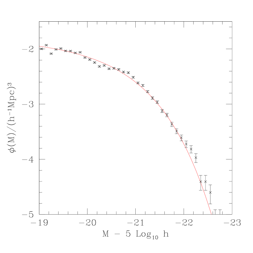
Figure 1: Luminosity function in the mock catalog (symbols with error bars); $M$ refers to the absolute magnitude in the $r-$band. Smooth curve shows the SDSS luminosity function (Blanton et al. 2003).

For reasons described by Sheth, Connolly & Skibba (2005), the marked correlation function we measure in the mock catalogs is

$$M(s)\equiv{1+W(s)\over 1+\xi(s)},$$ (4)

where $\xi(s)$ is the two-point correlation function in redshift space, and $W(s)$ is the same sum over galaxy pairs separated in redshift space by $s$, but now each member of the pair is weighted by the ratio of its luminosity to the mean luminosity of all the galaxies in the mock catalog. (Schematically, if the estimator for $1+\xi$ is $DD/RR$, then the estimator for $1+W$ is $WW/RR$, so the estimator we use for $M$ is $WW/DD$.) This measurement of $M(s)$ represents the prediction of the ‘standard’ model: the shape of the luminosity weighted correlation function includes the effects of the statistical correlation between halo mass and environment, but no other physical effects.

3 The halo model description

This section shows how to describe the marked correlation in redshift space discussed above in the language of the halo model. Details are in Skibba & Sheth (2005); in essence, the calculation combines the results of Sheth (2005) with those of Seljak (2001).

In the halo model, all mass is bound up in dark matter halos which have a range of masses. Hence, the density of galaxies is

$$\bar{n}_{\rm gal}=\int dm\,{dn(m)\over dm}\,N_{\rm gal}(m),$$ (5)

where $dn(m)/dm$ denotes the number density of haloes of mass $m$. The redshift space correlation function is the Fourier transform of the redshift space power spectrum $P(k)$:

$$\xi(s)=\int{dk\over k}\,{k^{3}P(k)\over 2\pi^{2}}\,{\sin ks\over ks}.$$ (6)

In the halo model, $P(k)$ is written as the sum of two terms: one that arises from particles within the same halo and dominates on small scales (the 1-halo term), and the other from particles in different haloes which dominates on larger scales (the 2-halo term). Namely,

$$P(k)=P_{1h}(k)+P_{2h}(k),$$ (7)

where, in redshift space,

$$P_{1h}(k) = \int dm\,{dn(m)\over dm}\,\Biggl{[}{2N_{\rm sat}(m)\,u_{1}(k|m)\over\bar{n}_{\rm gal}^{2}}$$ (8)

$$\qquad\qquad\qquad\qquad+\ {N_{\rm sat}^{2}(m)\,u_{2}^{2}(k|m)\over\bar{n}_{\rm gal}^{2}}\Biggr{]},$$

$$P_{2h}(k) = \left(F_{\rm g}^{2}+{2F_{\rm g}F_{\rm v}\over 3}+{F_{\rm v}^{2}\over 5}\right)\,P_{\rm Lin}(k),$$ (9)

$$u_{1}(k|m) = \left[{\sqrt{\pi}\over 2}{{\rm erf}(k\sigma_{\rm vir}(m)/\sqrt{2}H)\over k\sigma_{\rm vir}(m)/\sqrt{2}H}\right]\,u(k|m),$$ (10)

$$u^{2}_{2}(k|m) = \left[{\sqrt{\pi}\over 2}{{\rm erf}(k\sigma_{\rm vir}(m)/H)\over k\sigma_{\rm vir}(m)/H}\right]\,u^{2}(k|m),$$ (11)

$u(k|m)$ is the Fourier transform of the halo density profile divided by the mass $m$, $H$ is the Hubble constant, and

$$\sigma_{\rm vir}^{2}(m)\approx{Gm\over 2r_{\rm vir}}=G\left({\pi\over 6}m^{2}\Delta_{\rm vir}\bar{\rho}\right)^{1/3}$$ (12)

is the line-of-sight velocity dispersion within a halo ($\Delta_{\rm vir}\approx 200$). In addition, the bias factor $b(m)$ describes the strength of halo clustering,

$$F_{\rm v} = f\int{\rm d}m\,{{\rm d}n(m)\over{\rm d}m}\,{m\over\bar{\rho}}\,u_{1}(k|m)\,b(m),$$ (13)

$$F_{\rm g} = \int{\rm d}m\,{{\rm d}n(m)\over{\rm d}m}\,{1+N_{\rm sat}(m)u_{1}(k|m)\over\bar{n}_{\rm gal}}\,b(m),$$ (14)

$f\equiv d\ln D(a)/d\ln a\approx\Omega^{0.6}$, and $P_{\rm Lin}(k)$ is the power spectrum of the mass in linear theory. The real space power spectrum is given by setting the terms in square brackets in equations (10) and (11) for $u_{1}$ and $u_{2}$ to unity, and $F_{\rm v}\to 0$. When explicit calculations are made, we assume that the density profiles of halos have the form described by Navarro et al. (1996), so $u$ has the form given by Scoccimarro et al. (2001), and that halo abundances and clustering are described by the parameterization of Sheth & Tormen (1999).

To describe the effect of weighting each galaxy by its luminosity, let $W(r)$ denote the weighted correlation function, and ${\cal W}(k)$ its Fourier transform. Following Sheth, Abbas & Skibba (2004) and Sheth (2005), we write this as the sum of two terms:

$${\cal W}(k)={\cal W}_{1h}(k)+{\cal W}_{2h}(k),$$ (15)

where

$${\cal W}_{1h}(k) = \int dm\,{dn(m)\over dm}$$

$$\ \times\ \Biggl{[}{2L_{\rm cen}(m)\,\langle L|m,L_{\rm min}\rangle\,N_{\rm sat}(m)\,u_{1}(k|m)\over\bar{n}_{\rm gal}^{2}\ \bar{L}^{2}}$$

$$\qquad\qquad+\ {\langle L|m,L_{\rm min}\rangle^{2}N_{\rm sat}^{2}(m)\,u_{2}^{2}(k|m)\over\bar{n}_{\rm gal}^{2}\ \bar{L}^{2}}\Biggr{]},$$

$${\cal W}_{2h}(k) = \left(F_{\rm w}^{2}+{2F_{\rm w}F_{\rm v}\over 3}+{F_{\rm v}^{2}\over 5}\right)\,P_{\rm Lin}(k),$$

with

$$F_{\rm w} = \int{\rm d}m\,{{\rm d}n(m)\over{\rm d}m}\,b(m)\,$$ (16)

$$\quad\times\ {L_{\rm cen}(m)+N_{\rm sat}(m)\langle L|m,L_{\rm min}\rangle u_{1}(k|m)\over\bar{n}_{\rm gal}\ \bar{L}}$$

and

$$\bar{L}=\int dm\,{dn(m)\over dm}\,{L_{\rm cen}(m)+N_{\rm sat}(m)\,\langle L|m,L_{\rm min}\rangle\over\bar{n}_{\rm gal}}\,.$$ (17)

Here $\bar{L}$ is the average luminosity, $L_{\rm cen}(m)$ is the luminosity of the galaxy at the centre of an $m$-halo, and $\langle L|m,L_{\rm min}\rangle$ is the average luminosity of satellite galaxies more luminous than $L_{\rm min}$ in $m$-haloes. Thus, the calculation requires an estimate of how the central and the average satellite luminosity depend on $m$. As we show below, both are given by the luminosity dependence of $\xi$ (i.e., equation 1), so this halo model calculation of the weighted correlation function requires no additional information!

The luminosity of the central galaxy is obtained by inverting the relation between $M_{\rm min}$ and $L$ (e.g., equation 2). Obtaining an expression for the average luminosity of a satellite galaxy is more complicated. Define

$$P(>L|m,L_{\rm min}) \equiv {N_{\rm sat}(>L|m)\over N_{\rm sat}(>L_{\rm min}|m)}$$ (18)

$$= \int_{L}^{\infty}dL\,p(L|m,L_{\rm min}),$$

where $N_{\rm sat}$ is given by equation (1). Then the mean luminosity of satellites in $m$ halos,

$$\langle L|m,L_{\rm min}\rangle=\int_{L_{\rm min}}^{\infty}dL\,p(L|m,L_{\rm min})\,L,$$ (19)

can be obtained from the fact that

$$\int_{L_{\rm min}}^{\infty}dL^{\prime}\,P(>L^{\prime}|m,L_{\rm min}) = \langle L|m,L_{\rm min}\rangle-L_{\rm min}.$$ (20)

This shows that if we add $L_{\rm min}$ to the quantity on the left hand side (which is given by integrating equation 1 over $L$), we will obtain the quantity we are after.

Figure 2: Mean number of galaxies in a halo (top) and mean luminosity in a halo (bottom) for SDSS galaxies with $M_{r}<-20.5$, as a function of the masses of their parent halos, predicted by the luminosity dependence of clustering. Different curves in bottom panel show the mean luminosity of the galaxies in a halo, the luminosity of the central galaxy, and the mean luminosity of the others, as a function of halo mass (solid, dashed, and dotted curves). Symbols show the result of computing these relations in our mock catalogs.

Incidentally, since both $L_{\rm cen}(m)$ and $\langle L|m,L_{\rm min}\rangle$ can be estimated from the SDSS fits, the mean luminosity of the galaxies in an $m$-halo,

$$L_{\rm av}(m,L_{\rm min})={L_{\rm cen}(m)+N_{\rm sat}(m,L_{\rm min})\langle L|m,L_{\rm min}\rangle\over 1+N_{\rm sat}(m,L_{\rm min})},$$ (21)

is completely determined by equation (1). The mass-to-light ratio of an $m$ halo is $m/[N_{\rm gal}(m)\,L_{\rm av}(m)]$: this shows explicitly that the luminosity dependence of the galaxy correlation function constrains how the halo mass-to-light ratio must depend on halo mass. This halo-mass dependence has been used by Tinker et al. (2005); our analysis provides an analytic calculation of the effect. It shows that, in low mass halos, $L_{\rm av}\approx L_{\rm cen}$ because $N_{\rm sat}\ll 1$, whereas in massive halos, $L_{\rm av}<L_{\rm cen}$. Figure 2 compares the mass dependence of $L_{\rm av}$, $L_{\rm cen}$, and $L_{\rm sat}$ for galaxies restricted to $M_{r}<-20.5$ as predicted by Zehavi et al.’s (2005) halo model interpretation of the luminosity dependence of clustering in the SDSS. The symbols show measurements from our mock catalogs. The different quantities scale very differently with halo mass, with the following consequence.

Equation (15) treats the central galaxies differently from the others. If the luminosities of the central galaxies were not special, then the contribution to the one-halo term would scale as $N_{\rm sat}L_{\rm av}^{2}$ for the centre-satellite term, and $(N_{\rm sat}L_{\rm av})^{2}$ for the satellite-satellite term. Note that, in this case, the luminosity weights are the same for the two types of terms—only the number weighting differs. However, because the mass dependence of $L_{\rm av}$ is so different from that of the other two terms (cf. Figure 2), marked statistics allow one to discriminate between models which treat the central object as special from models which do not (e.g. Sheth 2005).

Figure 3: Luminosity-weighted real-space correlation function measured in a mock catalogs which resembles an SDSS volume limited sample with $M_{r}<-20.5$. Symbols show the measurements; smooth curves show the associated halo-model predictions when the luminosity of the central galaxy in a halo is assumed to be different from the others; dashed curves show the prediction when the central object is not special. Dotted curves show the mean and rms values of the statistic $M$, obtained by after randomizing the marks and remeasuring $M$ one hundred times.

To illustrate, the symbols in the top and bottom panels of Figure 3 show measurements of $\xi(r)$ and $M(r)$ measured in this mock catalog. Error bars were obtained with a “jack-knife” procedure, as detailed in Scranton et al. (2002), in which the statistic is re-measured after omitting a random region, and repeating thirty times ($\sim$1.5 times the number of bins in separation for which we present results). Note that the errors in $W$ are strongly correlated with those in $\xi$, so that the true error in $M$ is grossly (more than a factor of ten) overestimated if one simply sums these individual errors in quadrature. A much better approximation of the uncertainties is obtained as follows. Randomly scramble the marks among the galaxies, remeasure $M$, and repeat many ($\sim 100$) times. Compute the mean of $M$ over these realizations. This mean, and the rms scatter around it are shown as dotted lines in the two panels. Note that this scatter is within a factor of two of the full jackknife error estimate; it is smaller than the jackknife estimate on scales $r>1h^{-1}$Mpc and $s>3h^{-1}$Mpc, and, on smaller scales, it is larger than the jackknife estimate.

The solid lines in the top panel show the halo model calculation of $\xi$. These show that the model is in excellent agreement with the measurements on all scales in real space. The solid and dashed curves in the bottom panel show the associated halo model calculations of the marked statistic $M$ when central galaxies are special (solid), and when they are not (dashed). Note that both these curves give the same prediction for the unweighted statistic $\xi$.

Comparison of these curves with the measurements yields two important pieces of information. First, on large scales ($r>4h^{-1}$Mpc), the solid and dashed curves are identical, and they are in excellent agreement with the measurements. This indicates the large-scale signal is well described by a model in which there are no additional correlations with environment other than those which arise from the correlation between halo mass and environment. This is not reassuring, since the mock catalogs were constructed to have no correlations other than those which are due to halo bias. Second, on smaller scales, the solid curves are in substantially better agreement with the measurements than are the dashed curves. (A $\chi^{2}$ estimate of the goodness of fit of the two marked correlation models yields values which smaller by a factor of ten when the central galaxy is treated specially compared to when it is not.) Since the mock catalogs do treat the central galaxies differently from the others, it is reassuring that the halo model calculation which incorporates this difference is indeed in better agreement with the measurements.

Figure 4: Luminosity-weighted redshift-space correlation functions measured in mock catalogs which resemble an SDSS volume limited sample with $M_{r}<-20.5$. Symbols show the measurements; smooth curves show the associated halo-model predictions when the luminosity of the central galaxy in a halo is assumed to be different from the others; dashed curves show the prediction when the central object is not special. Dotted curves show the mean and rms values of the statistic $M$, obtained by after randomizing the marks and remeasuring $M$ one hundred times. Dot-dashed curves in show the one- and two-halo contributions to the statistic in our model when the central object in a halo is special.

In the next section, we will present measurements of marked statistics in redshift space. To see if we can use our halo model calculation to interpret the measurements, Figure 4 compares measurements of $\xi(s)$ and $M(s)$ in the mock catalog with our halo model calculation. The format is similar to Figure 3: solid curves in the bottom panels show the predicted marked statistic $M$ when the central galaxy in a halo is treated differently from the others, and dashed curves show what happens if it is not. Both curves give the same prediction for the unweighted statistic $\xi$.

The top panel shows that the halo model calculation of $\xi(s)$ is in excellent agreement with the measurements on scales larger than a few Mpc, as it was for $\xi(r)$. However, it is not as accurate when the redshift separations are of order a few Mpc. Nevertheless, the model is able to reproduce the factor of ten difference between $\xi(r)$ and $\xi(s)$ on small scales. We will discuss the reason for the discrepancy on intermediate scales shortly.

Similarly, the bottom panel shows excellent agreement between measurements and model for the marked statistic $M(s)$ on large scales ($s>8h^{-1}$Mpc), both when the central object is treated specially and when it is not. In addition, the model in which the central object is special is in better agreement with the measurements on small scales. (A $\chi^{2}$ estimate of the goodness of fit of the two marked correlation models yields values which smaller by more than a factor of two when the central galaxy is treated specially compared to when it is not.) On intermediate scales, however, there is substantial discrepancy discrepancy between the model and the mocks; the discrepancy is more pronounced for $M(s)$ than for $\xi(s)$.

To study the cause of this discrepancy, dot-dashed lines show the two contributions to the statistic, ${\cal W}_{1h}/(1+\xi)$ and $(1+{\cal W}_{2h})/(1+\xi)$, separately. This shows that it is on scales where both terms contribute that the model is inaccurate. There are two reasons why it is likely that this inaccuracy can be traced to our simple treatment of the two-halo term. The suppression of power due to virial motions means that we must model the two-halo term more accurately in redshift-space than in real-space. Our halo-model calculation incorrectly assumes that linear theory is a good approximation even on small scales (e.g. Scoccimarro 2004 shows that this is a dangerous assumption even on scales of order 10 Mpc) and that volume exclusion effects (Mo & White 1996) are negligible (Sheth & Lemson 1999 discuss how one might incorporate such effects). Because our mocks make use of both the positions and velocities of the halos in the simulations, they incorporate both these effects. Thus, our simple halo-model likely underestimates $M(s)$ on intermediate scales, but overestimates it on smaller scales. Since this is in the sense of the discrepancy with the measurements in the mock catalogs, it is likely that this inaccuracy can be traced to our simple treatment of the two-halo term. We will have cause to return to this discrepancy in the next section, where we use our halo model calculation to interpret measurements of marked statistics in the SDSS dataset.

4 Measurements in the SDSS

Figure 5 shows $\xi(r_{p},\pi)$ and $W(r_{p},\pi)$, the unweighted (solid) and weighted (dashed) correlation functions of pairs with separations $r_{p}$ and $\pi$, perpendicular and parallel to the line of sight. The measurements were made in a volume limited catalog (59,293 galaxies with $M_{r}<-20.5$) extracted from the SDSS DR4 database (Adelman-McCarthy et al. 2005). Contours show the scales at which the correlation functions have values of 0.1, 0.2, 0.5, 1, 2, and 5, when averaged over bins of $2h^{-1}$Mpc in $r_{p}$ and $\pi$. This format, due to Davis & Peebles (1983), allows one to isolate redshift space effects on the correlation functions, since these act only in the $\pi$ direction. The dotted quarter circles at separations of 5, 10 and $20h^{-1}$Mpc are drawn to guide the eye—they serve to highlight the fact that both $\xi(r_{p},\pi)$ and $W(r_{p},\pi)$ are very anisotropic. In constrast, the corresponding real-space quantities would be isotropic. The figure shows clearly that $W$ has a slightly higher amplitude than $\xi$ on the scales shown.

Figure 5: Unweighted (solid) and weighted (dashed) correlation functions measured in volume limited catalog with $M_{r}<-20.5$ in the SDSS. Dotted curves show that the measured correlation functions are significantly anisotropic.

The quantity studied in the previous section, for which we have analytic (halo-model) estimates, can be derived from this plot as follows. Counting pairs in spherical shells of radius $s=\sqrt{r_{p}^{2}+\pi^{2}}$ yields the redshift space correlation function $\xi(s)$. This measure of clustering is sensitive to the fact that the correlation function in redshift-space is anisotropic; in particular, it contains information about the typical motions of galaxies within halos (which are responsible for the elongation of the contours along the $\pi$ direction at $r_{p}\leq 5h^{-1}$ Mpc), as well as the motions of the halos themselves (which are responsible for the squashing along the $\pi$ direction at $r_{p}\geq 5h^{-1}$ Mpc). The result of counting pairs of constant $r_{p}$, whatever their value of $\pi$, yields the projected correlation function $w_{p}(r_{p})$; since $r_{p}$ is not affected by redshift space distortions, this quantity contains no information about galaxy or halo motions, so is more closely related to the real-space correlation function. Figures 6 and 7 compare both these quantities with the corresponding halo-model calculations.

Figure 6: Redshift-space correlation functions measured in volume limited catalogs with $M_{r}<-19.5$ (left) and $M_{r}<-20.5$ (right) in the SDSS. Top panels show the unweighted correlation function $\xi(s)$, and bottom panels show the marked statistic $M(s)$. Smooth curves show the associated redshift-space halo-model predictions; solid curves are when the central galaxy in a halo is treated differently from the others, whereas this is not done for the dashed curves. Dotted curves show the mean and rms values of the statistic $M$, estimated by randomizing the marks and remeasuring $M$ one hundred times. Two sets of curves are shown in the right hand panels; the top set of solid and dashed curves shows the halo model calculation in which the relation between the number of galaxies and halo mass is given by equation (1), and the bottom set follow from equation (3).

Figure 6 shows $\xi(s)$ and $M(s)$ measured in two volume limited catalogs extracted from the SDSS database. One of these catalogs is the same as that which resulted in Figure 5, and the other is for a slightly fainter sample ($M_{r}<-19.5$, with 61,821 galaxies). Error bars are estimated by jack-knife resampling, as discussed previously. The solid curves show the redshift-space halo-model calculation in which central galaxies are special, and dashed curves show the expected signal if they are not. (Recall that both have the same $\xi(s)$.)

On large scales, both the solid and dashed curves provide an excellent description of the measurements on large scales. This agreement suggests that correlations with environment on scales larger than a few Mpc are entirely a consequence of the correlation between halo abundances and environment, just as they were in the mock catalogs. Since the model calculation incorporates the assumption that the halo mass function is top-heavy in dense regions, the agreement with the measured $M(s)$ provides strong evidence that this is indeed the case.

The discrepancy between the halo-model calculation and the measurements on intermediate scales is similar to the discrepancy between the halo-model and the mock catalogs studied in the previous section. There we argued that this is almost certainly due to our simple treatment of the two-halo contribution to the statistic. Indeed, the marked statistics in the mock catalogs behave qualitatively like those in the SDSS data (compare Figures 4 and 6), suggesting that the discrepancy between the halo-model calculation and the measurements are due to this, rather than to any environmental effects operating on intermediate scales.

Figure 7: Projected correlation function measured in volume limited catalog with $M_{r}<-20.5$ in the SDSS. Top panel shows the unweighted projected correlation function $w_{p}(r_{p})$, and bottom panels show the marked statistic $M_{p}(r_{p})$. Smooth curves show the associated projected halo-model predictions; solid curves are when the central galaxy in a halo is treated differently than the others, whereas this is not done for the dashed curves. The upper set of dashed and solid curves show halo-model calculations which follow from equation (1); the lower set of curves assume equation (3).

On small scales, the solid curves are in substantially better agreement with the data than are the dashed curves ($\chi^{2}$ smaller by a factor of four in both plots). Evidently, central galaxies are indeed a special population in the data. This provides substantial support for the assumption commonly made in halo-model interpretations of the galaxy correlation function that the central galaxy in a halo is different from all the others.

However, even the solid curves are not in particularly good agreement with the measurements. Before attributing the discrepancy to environmental effects not included in the halo model description, we have explored the effect of modifying our parametrization of the relation between the number of galaxies and halo mass which we use (equation 1). Figure 6 shows that the parametrization in equation (3), with $\sigma=0.5$ and $M_{1}/M_{\rm min}=30$, provides equally good fits to $\xi(s)$, but a slightly better description of $M(s)$. In this parameterization of the scaling of $N_{\rm gal}$ with halo mass, the minimum halo mass required to host a galaxy is not a sharp step function.

Further evidence in support of the parametrization in which the minimum mass cutoff is not sharp, and in which the central galaxy is different from the others is shown in Figure 7. The top and bottom panels compare measurements of the projected correlation functions $w_{p}(r_{p})$ and $M_{p}(r_{p})$, where

$$w_{p}(r_{p}) = \int{\rm d}y\,\xi(r_{p},y)=2\int_{r_{p}}^{\infty}{\rm d}r\,{r\,\xi(r)\over\sqrt{r^{2}-r_{p}^{2}}},\quad{\rm and}$$

$$M_{p}(r_{p}) = {1+W_{p}(r_{p})/r_{p}\over 1+w_{p}(r_{p})/r_{p}},\qquad{\rm where}$$

$$W_{p}(r_{p}) = 2\int_{r_{p}}^{\infty}{\rm d}r\,{r\,W(r)\over\sqrt{r^{2}-r_{p}^{2}}}\ {\rm and}\ r=\sqrt{r_{p}^{2}+y^{2}},$$ (22)

with the associated halo-model calculations. (In the halo model, the real-space quantities $\xi(r)$ and $W(r)$ which appear in the expressions above, are related to $\xi(s)$ and $W(s)$ by setting setting $F_{\rm v}=0$ and taking the limit $\sigma_{\rm vir}\to 0$ in $u_{1}$ and $u_{2}$. See Skibba & Sheth 2006 for our particular definition of $M_{p}$.) Note that these projected quantities are free of redshift space distortions, making them somewhat easier to interpret.

As was the case for the redshift space measurements, both parameterizations of $N_{\rm gal}(M)$ provide good descriptions of the unweighted statistic $w_{p}(r_{p})$, and in both cases, the weighted statistic is in better agreement when the central object is treated specially. However, the Figure shows clearly that when the central object is special, then equation (3) provides a substantially better description of $M_{p}$—the agreement with the measurements is excellent over all scales.

5 Discussion

We showed how to generate a mock galaxy catalog which has the same luminosity function (Figure 1) and luminosity dependent two-point correlation function as the SDSS data. We used the mock catalog to calculate the luminosity-weighted correlation function in a model where all environmental effects are a consequence of the correlation between halo mass and environment (Figures 3 and 4 show results in real and redshift space). We then showed how to describe this luminosity-weighted correlation function in the language of the redshift-space halo model (equation 15). The analysis showed that estimates of the luminosity dependence of clustering constrain how the mass-to-light ratio of halos depends on halo mass (equation 21 and Figure 2). The central galaxy in a halo is predicted to be substantially brighter than the other objects in the halo, and although the luminosity of the central object increases rapidly with halo mass, the mean luminosity of the other objects in the halo is approximately independent of the mass of the host halo.

Our analysis also showed that measurements of clustering as a function of luminosity completely determine the simplest halo model description of marked statistics. In addition, measurements of the marked correlation function allow one to discriminate between models which treat the central object in a halo as special, from those which do not (Figures 3 and 4). Also, in hierarchical galaxy formation models, the marked correlation function is expected to show a signal on large scales if the average mark of the galaxies in a halo correlates with halo mass. The signal arises because massive halos populate the densest regions; it is present even if there are no physical effects which operate to correlate the marks over large scales.

We compared this halo model of marked statistics with measurements in the SDSS (Figures 6 and 7). The agreement between the model and the measurements on scales smaller than a few Mpc provides strong evidence that central galaxies in halos are a special population—in general, the central galaxy in a halo is substantially brighter than the others. (Berlind et al. 2004 come to qualitatively similar conclusions, but from a very different approach.) Substantially better agreement is found for a model in which the minimum halo mass required to host a luminous central galaxy does not change abruptly with luminosity. This is in qualitative agreement with some semi-analytic galaxy formation models, which generally predict some scatter in central luminosity at fixed halo mass (e.g. Sheth & Diaferio 2001; Zheng et al. 2005).

The agreement between the halo model calculation and the data on scales larger than a few Mpc indicates that the standard assumption in galaxy formation models, that halo mass is the primary driver of correlations between galaxy luminosity and environment, is accurate. In particular, these measurements are consistent with a model in which the halo mass function in large dense regions is top-heavy, and, on these large scales, there are no additional physical or statistical effects which affect the luminosities of galaxies. In this respect, our conclusions are similar to those of Mo et al. (2004), Kauffmann et al. (2004), Blanton et al. (2005), and Abbas & Sheth (2006), although our methods are very different.

We note in passing that there is a weak statistical effect for which the halo-model above does not account: at fixed mass, haloes in dense regions form earlier (Sheth & Tormen 2004). Gao, Springel & White (2005) show that this effect is more pronounced for low mass haloes (related marked correlation function analyses by Harker et al 2006 and Wechsler et al. 2006 come to similar conclusions). The agreement between our halo-model calculation and the measurements in the SDSS suggests that this correlation between halo formation and environment is not important for the relatively bright galaxy population we have studied here. This is presumably because these SDSS galaxies populate more massive haloes. Comparisons with larger upcoming SDSS datasets, with a fainter luminosity threshold (such as $M_{r}<-18$), may bear out the correlation between low-mass halo formation and environment.

As a final indication of the information contained in measurements of marked statistics, Figure 8 compares $M(s)$ when the $u-$, $g-$ and $r-$band luminosities are used as the mark. The underlying population is the same as that for Figures 5–7: the sample is volume limited to $M_{r}<-20.5$. Thus, $\xi(s)$ is fixed, and only $W(s)$ changes with wave-band. Notice that there is a clear trend with wavelength: there is a slight anti-correlation in the $u-$band, whereas $M(s)$ rises slightly with decreasing scale when $g-$band luminosity is the mark, and the signal is even stronger when $L_{r}$ is the mark. This trend with wavelength is qualitatively consistent with the predictions of semi-analytic galaxy formation models (Sheth, Connolly & Skibba 2005) and indicates that the mean $u$-band luminosity of the galaxies in a halo depends less strongly on halo mass than does the mean $r-$band luminosity in a halo (Sheth 2005). In the models, the $u-$band luminosity is an indicator of the star formation rate; our measurements suggest that the correlation between star formation rate and halo mass is weak—if it is an increasing function of halo mass at low masses, then it decreases at larger masses.

Figure 8: Redshift-space luminosity-weighted correlation functions measured in volume limited catalogs with $M_{r}<-20.5$ in the SDSS. Circles, triangles and squares show $M(s)$ when the weight is $r-$, $g-$ and $u-$band luminosity respectively. For clarity, jack-knife error bars are only shown for the $r-$band measurement, since the uncertainties are similar in the other bands.

Figure 9 shows the result of weighting these same galaxies by their colors. The top panel shows results where the weight is the difference in the absolute magnitudes, $M_{u}-M_{r}$ and $M_{g}-M_{r}$, whereas the weights in the bottom bottom panel were the ratios of the luminosities in two bands. Comparison of the two panels shows the effect on $M(s)$ of rescaling the weights while preserving their rank-ordering—while there are quantitative differences, the results in both panels are qualitatively similar. The $M(s)$ measurements shown in the bottom panel are more widely separated because the luminosity ratio involves $10^{\rm color}$, which has the effect of weighting the redder galaxies more heavily. In particular, this analysis indicates clearly that close pairs of galaxies tend to be redder than average. Sheth, Connolly & Skibba (2005) show that this is also the case in semi-analytic galaxy formation models.

The measurements shown in Figures 8 and 9 are consistent with models in which galaxies in clusters are more massive and have smaller star formation rates than galaxies in the field. In effect, these figures demonstrate the environmental dependence of galaxy luminosities and colors, without having to divide the galaxy sample up into discrete bins of ‘field’, ‘group’, and ‘cluster’. Thus, marked statistics allow one to study correlations with environment over a continuous range in density, rather than in somewhat arbitrary discrete bins in environment. In this respect, our use of marked statistics to quantify and interpret environmental trends is very different from recent approaches which address the same problem. Since marked statistics are simple to measure and interpret, we hope that they will become standard tools for quantifying the correlation between the properties of galaxies and their environments.

Figure 9: Redshift-space color-weighted correlation functions measured in volume limited catalogs with $M_{r}<-20.5$ in the SDSS. The top panel shows results when the color weight is the difference in absolute magnitudes. In the bottom panel, galaxies were weighted by the ratio of the luminosities in the two bands, so they span a greater range around the mean value. Both panels show that close pairs of galaxies tend to have redder colors, although the difference is clearer when the weights span a greater range around the mean value.

References

- [1] Abbas U., Sheth R. K., 2006, MNRAS, submitted
- [2] Adelman-McCarthy et al., 2005, ApJS, in press (astro-ph/0507711)
- [3] Beisbart C., Kerscher M., 2000, ApJ, 545, 6
- [4] Berlind A. B., Blanton M. R., Hogg D. W., Weinberg D. H., Dave R., Eisenstein D. J., Katz N., 2005, ApJ, 629, 625
- [5] Blanton M. R. et al. 2003, ApJ, 592, 819
- [6] Blanton M. R., Eisenstein D. J., Hogg D. W., Zehavi I., 2005, ApJ, submitted (astro-ph/0411037)
- [7] Cooray A., Sheth R. K., 2002, Phys. Rep., 372, 1
- [8] Davis M., Peebles P. J. E., 1983, ApJ, 267, 465
- [9] Gao L., Springel V., White S. D. M., 2005, MNRAS, 363, 66
- [10] Harker G., Cole S., Helly J., Frenk C. S., Jenkins A., 2006, MNRAS, submitted (astro-ph/0510488)
- [11] Kauffmann G., Diaferio A., Colberg J., White S. D. M., 1999, MNRAS, 303, 188
- [12] Kauffmann G. A. M., White S. D. M., Heckman T. M., Ménard B., Brinchmann J., Charlot S., Tremonti C., Brinkmann J., 2004, MNRAS, 353, 713
- [13] Kravtsov A., et al., 2004, ApJ, 609, 35
- [14] Mo H. J., White S. D. M., 1996, MNRAS, 282, 347
- [15] Mo H. J., Yang X., van den Bosch F. C., Jing Y. P., 2004, MNRAS, 349, 205
- [16] Navarro J., Frenk C., White S. D. M., 1996, ApJ, 462, 563
- [17] Scranton et al., 2002, ApJ, 579, 48
- [18] Sheth R. K., 2005, MNRAS, 364, 796
- [19] Sheth R. K., Abbas U., Skibba R. A., in Diaferio A., ed, Proc. IAU Coll. 195, Outskirts of galaxy clusters: intense life in the suburbs, CUP, Cambridge, p. 349
- [20] Sheth R. K., Connolly A. J., Skibba R., 2005, MNRAS, submitted
- [21] Sheth R. K., Diaferio A., 2001, MNRAS, 322, 901
- [22] Sheth R. K., Tormen G., 1999, MNRAS, 308, 119
- [23] Sheth R. K., Tormen G., 2002, MNRAS, 329, 61
- [24] Sheth R. K., Tormen G., 2004, MNRAS, 350, 1385
- [25] Skibba R., Sheth R. K., 2005, MNRAS, in preparation
- [26] Stoyan D., Stoyan H., 1994, Fractals, Random Shapes, and Point Fields. Wiley & Sons, Chichester
- [27] Tinker J. L., Weinberg D. H., Zheng Z., Zehavi I., ApJ, 631, 41
- [28] Wechsler R. H., Zentner A. R., Bullock J. S., Kravtsov A. V., 2006, ApJ, submitted (astro-ph/0512416)
- [29] York D., et al., 2000, AJ, 120, 1579
- [30] Zehavi I., et al., 2005, ApJ, 630, 1
- [31] Zheng Z., et al., 2005, ApJ, 633, 791