Measuring Stellar Velocity Dispersions in Active Galaxies

Abstract

We present stellar velocity dispersion ($\sigma_{\ast}$) measurements for a significant sample of 40 broad-line (Type 1) active galaxies for use in testing the well-known relation between black hole mass and stellar velocity dispersion. The objects are selected to contain Ca II triplet, Mg I$b$ triplet, and Ca H+K stellar absorption features in their optical spectra so that we may use them to perform extensive tests of the systematic biases introduced by both template mismatch and contamination from the active galactic nucleus (AGN). We use the Ca II triplet as a benchmark to evaluate the utility of the other spectral regions in the presence of AGN contamination. Broad Fe II emission, extending from $\sim 5050-5520$ Å, in combination with narrow coronal emission lines, can seriously bias $\sigma_{\ast}$ measurements from the Mg I$b$ region, highlighting the need for extreme caution in its use. However, we argue that at luminosities constituting a moderate fraction of the Eddington limit, when the Fe II lines are both weak and smooth relative to the stellar lines, it is possible to derive meaningful measurements with careful selection of the fitting region. In particular, to avoid the contamination of coronal lines, we advocate the use of the region 5250–5820 Å, which is rich in Fe absorption features. At higher AGN contaminations, the Ca H+K region may provide the only recourse for estimating $\sigma_{\ast}$. These features are notoriously unreliable, due to a strong dependence on spectral type, a steep local continuum, and large intrinsic broadening. Indeed, we find a strong systematic trend in comparisons of Ca H+K with other spectral regions. Luckily the offset is well-described by a simple linear fit as a function of $\sigma_{\ast}$, which enables us to remove the bias, and thus extract unbiased $\sigma_{\ast}$ measurements from this region. We lay the groundwork for an extensive comparison between black hole mass and bulge velocity dispersion in active galaxies, as described in a companion paper by Greene & Ho.

1 Introduction

It has long been known that some galaxies harbor supermassive black holes (BHs) at their centers, whose accretion-powered luminosity may outshine their entire host galaxy (e.g., Lynden-Bell 1969). More recently, we have learned that most, if not all, galaxies with a bulge contain central BHs (Kormendy & Richstone 1995; Magorrian et al. 1998; Ho 1999), whose masses are tightly correlated with the stellar velocity dispersion ($\sigma_{\ast}$) of the bulge (the $M_{\mathrm{BH}}-\sigma_{\ast}$ relation: Ferrarese & Merritt 2000; Gebhardt et al. 2000a; Tremaine et al. 2002). It is likely that the $M_{\mathrm{BH}}-\sigma_{\ast}$ relation is established during the active galactic nucleus (AGN) phase of a galaxy’s life-cycle, since energy emitted by the BH may simultaneously limit the gas supply for building both the bulge and the BH itself (e.g., Silk & Rees 1998). If we are to understand this critical stage in galaxy evolution, we must have robust methods to estimate both BH masses and $\sigma_{\ast}$ in active galaxies.

Reverberation mapping (Blandford & McKee 1982) is currently the most direct way to obtain BH masses in AGNs, although the masses are uncertain by a factor that depends on the poorly constrained geometry of the broad-line region (BLR). Reverberation mapping provides an estimate of the size of the BLR from the lag between the variability in the photoionizing continuum and the broad emission lines. With a BLR size at hand, one can infer a virial mass for the very central region of the AGN, and hence for the BH (Ho 1999; Wandel et al. 1999; Kaspi et al. 2000; Peterson et al. 2004): $M_{\mathrm{BH}}$ = $fR_{\mathrm{BLR}}v^{2}/G$, where $v$ is the velocity dispersion of the BLR gas and the factor $f$ accounts for the geometry of the BLR (e.g., Onken et al. 2004; Kaspi et al. 2005). For instance, a spherical BLR has an $f$ value of 0.75 when $v$ is measured using the full width at half-maximum (FWHM) of the broad line (e.g., Netzer 1990). Reverberation mapping has further been used to derive an empirical relation between AGN luminosity and BLR radius (the radius-luminosity relation): $R_{\mathrm{BLR}}$ $\propto L_{5100\AA}^{0.6-0.7}$ (Kaspi et al. 2000, 2005; Greene & Ho 2005b). Since reverberation mapping data are time-consuming to obtain, and are currently available only for a small number of objects, practical applications of the virial technique to estimate BH masses have relied on the radius-luminosity relation and BLR line widths measured from single-epoch spectra (e.g., McLure & Dunlop 2001; Vestergaard 2002; Greene & Ho 2004). Given the many uncertainties inherent in the virial technique (see Krolik 2001 for a detailed discussion), in particular the unknown geometry of the BLR, one may justifiably question its reliability. On the other hand, Gebhardt et al. (2000b) and Ferrarese et al. (2001) showed that virial BH mass estimates agree surprisingly well with masses inferred from the $M_{\mathrm{BH}}-\sigma_{\ast}$ relation, at least for a handful of objects. Subsequent work (Nelson et al. 2004; Onken et al. 2004) has increased the sample size, still considering a total of only 17 objects between the two samples. Onken et al. find that reverberation mapped masses, using the standard assumption of a spherical BLR and the FWHM, are $\sim 0.26$ dex below the masses inferred from the Tremaine et al. (2002) fit to the $M_{\mathrm{BH}}-\sigma_{\ast}$ relation; Nelson et al. obtain essentially the same result, concluding that the AGN sample lie systematically below the sample of inactive galaxies by 0.21 dex. However, as noted by Nelson et al., the significance of the measured offset is low, given the large scatter (0.46 dex) in the data. Since this value represents the zeropoint in the BH mass scale for AGNs, many more $\sigma_{\ast}$ measurements are required to improve the calibration. An enlarged sample would allow us to resolve outstanding technical questions, such as whether the FWHM or the actual second moment of the broad-line profile is a better measure of BLR velocity dispersion (e.g., Vestergaard 2002; Peterson et al. 2004), as yet unaddressed for virial masses obtained with single-epoch spectra. Furthermore, we would be able to explore the importance of BLR geometry in a statistical way, both by addressing the possible importance of inclination (e.g., McLure & Dunlop 2001) and by obtaining a more secure empirical measure of $f$. The BLR geometry may even depend on properties of the system such as BH mass and accretion rate. With such calibrations in hand, we may begin to address other fundamental questions, such as whether the $M_{\mathrm{BH}}-\sigma_{\ast}$ relation varies as a function of BH mass (e.g., Robertson et al. 2005) or evolves with time (e.g., Shields et al. 2003).

The primary hurdle in this endeavor lies with the difficulty of obtaining reliable $\sigma_{\ast}$ measurements in active galaxies. AGNs are bright, and thus detectable to cosmological distances, but the strong continuum of Type 1 sources dilutes the starlight while their rich emission-line spectrum confuses and distorts the shape of the stellar absorption features. This paper presents a comprehensive discussion of how to tackle this problem. Using a relatively large sample of AGNs for which we can measure $\sigma_{\ast}$ reliably, we discuss the relative merits and complications of measuring $\sigma_{\ast}$ from different spectral regions. The sample is described in §2. Section 3 introduces the direct-fitting code we have developed for measuring $\sigma_{\ast}$ and discusses the battery of tests to which we have subjected it to evaluate its robustness and limitations. The many challenges inherent in dealing with AGN spectra are outlined in §4, where we devote considerable attention to finding the optimal spectral regions for measuring $\sigma_{\ast}$ under realistic conditions encountered in AGNs. We end with some practical suggestions to serve as a guide for other researchers (§5), followed by a summary (§6). A companion paper (Greene & Ho 2005c) uses the final measurements obtained from this analysis to provide a new appraisal of the $M_{\mathrm{BH}}-\sigma_{\ast}$ relation of AGNs.

Throughout we assume the following cosmological parameters to calculate distances: $H_{0}=100~{}h=71$ km s^-1 Mpc^-1, $\Omega_{\rm m}=0.27$, and $\Omega_{\Lambda}=0.75$ (Spergel et al. 2003).

2 The Sample

We utilize the large and homogeneous database provided by the Sloan Digital Sky Survey (SDSS; York et al. 2000), which will eventually obtain imaging and follow-up spectroscopy for about one-quarter of the sky. Briefly, spectroscopic candidates are selected based on multi-band imaging (Strauss et al. 2002) with a drift-scan camera (Gunn et al. 1998). A pair of spectrographs is fed by $3\arcsec$-diameter fibers, covering $\sim 3800-9200$ Å with an instrumental resolution of $\lambda/\Delta\lambda\approx 1800$ (Gaussian $\sigma_{\rm inst}\approx 70$ km s^-1). The spectroscopic pipeline performs basic image calibrations, as well as spectral extraction, sky subtraction, removal of atmospheric absorption bands, and wavelength and spectrophotometric calibration (Stoughton et al.  2002). Finally, spectral classification is performed using cross-calibration with stellar, emission-line, and active galaxy templates. The Third Data Release (DR3; Abazajian et al. 2005) of SDSS contains 45,260 spectroscopically identified AGNs with $z<2.3$.

Sample spectral fits for the regions around (left column) the Ca II $\lambda\lambda$ 8498, 8542, 8662 triplet, (middle column) the Mg Ib $\lambda\lambda$5167, 5173, 5184 triplet, and (right column) Ca H+K $\lambda\lambda$3969, 3934. The top four rows are objects from our sample; the official SDSS name is given in the upper left-hand corner for each row. All spectra are shown at rest wavelengths and have been normalized to their local continua. The shaded areas denote regions that were excluded from the fit. For each object, the top spectrum is the galaxy spectrum, the middle spectrum is our best-fit template model (offset for clarity), and the bottom spectrum is the residuals. Note that the CaT features are much less diluted than Mg Ib. In the Mg Ib region we have only fit the range 5250–5820 Å, but we include the Mg Ib features to specifically highlight their high level of AGN dilution and Fe II contamination. In the Ca H+K region the entire H line needs to be masked from the fit. The bottom row shows the templates used in the analysis: the average stellar template, the A star template, and the Fe template derived from I Zw 1 (see text for details). The current Fe template does not extend to the CaT region, but Fe II emission is known to be weak in this region for AGNs (e.g., Persson 1988).

There are a limited number of optical stellar spectral features that have high enough equivalent width (EW) to be visible even in the presence of significant AGN contamination (see Fig. 1). The most common spectral regions employed are either around the Ca II $\lambda\lambda$8498, 8542, 8662 triplet (hereafter CaT) or the Mg Ib $\lambda\lambda$5167, 5173, 5184 triplet. Since we plan to compare various spectral regions, we select all spectroscopically identified AGNs from DR3 with $z\leq 0.05$, such that at least two of the three CaT lines are in the band. Of the 66 objects satisfying this criterion, we limit our attention to those with Ca II $\lambda 8542$ EW $\geq$ 1.5 Å and a local signal-to-noise ratio (S/N) of 18 or higher per pixel. On inspection, we rejected nine candidates meeting these requirements because of confusion from either Paschen or O I $\lambda 8446$ emission features or strong night-sky line residuals, leaving a final sample of 40 objects (Table 1).

3 Stellar Velocity Dispersion Measurements

3.1 The Method

Depending on the application, a variety of methods are used to measure stellar velocity dispersions. Those involving Fourier techniques include cross-correlation (Tonry & Davis 1979), the Fourier quotient (Simkin 1974; Sargent et al. 1977), and the Fourier correlation quotient (Bender 1990). The use of Fourier space is natural, as velocity broadening is reduced to a multiplication, making the methods computationally cheap. It is also possible, however, to compare a grid of broadened template spectra directly with the galaxy spectrum in pixel space (Burbidge et al. 1961). While direct-fitting is comparatively computationally expensive, it is not particularly demanding by modern standards. There are many advantages to direct-fitting, as described, for example, by Rix & White (1992). Since the quality of the fit is measured in pixel space, error analysis and the effects of noise are easily incorporated, as is the masking of corrupted spectral regions or emission lines. Furthermore, AGN features are easily incorporated as additional model components in a direct fit. Following Barth et al. (2002a), we build a model, $M(x)$, that is the convolution of a stellar template spectrum, $T(x)$, and a line-of-sight velocity broadening function approximated as a Gaussian, $G(x)$:

$$M(x)=P(x)~{}\{[T(x)~{}\otimes\ G(x)]+C(x)\}.$$ (1)

The spectra and templates are normalized to the local continuum using identical spectral regions free of strong emission lines. We assume a Gaussian velocity broadening function for simplicity, but technically it is possible to solve for higher-order moments of the velocity profile (e.g., Rix & White 1992; van der Marel 1994). In our case the data quality does not warrant such a treatment. $C(x)$ is a model for the AGN continuum, here assumed to be a single power law, where both the normalization and slope are allowed to vary in the fit. This component could comprise other additive components, such as the Fe II emission from the BLR of the AGN that forms a “pseudo-continuum” throughout the optical spectrum (e.g., Francis et al. 1991). The polynomial factor, $P(x)$, is required to account for variations in continuum shape between the template and the galaxy (see, e.g., Kelson et al. 2000), which, in our case, can result from a combination of internal reddening in the host galaxy (Galactic extinction is already accounted for), differing stellar populations, and residual calibration errors. We typically use a third-order Legendre polynomial. Altogether, in addition to the velocity dispersion, we solve for the velocity shift, an amplitude and slope for the power-law component, and four polynomial components, for a total of eight free parameters. The best-fit parameters are determined through a minimization of the $\chi^{2}$ statistic using the non-linear Levenberg-Marquardt minimization algorithm as implemented by mpfit in IDL.

For stellar templates, we use 32 G and K giant stars in the old open cluster M67 observed with SDSS (see Bernardi et al. 2003). While the use of field stars is far more common, these templates are preferable because they are observed in an identical manner as the program objects. The near-solar metallicity of M67 ([Fe/H] = $-$0.05$\pm 0.03$; Montgomery et al. 1993) means that template mismatch problems resulting from metallicity (discussed below) are comparable to those expected from field stars. Note that we are using a restricted range of stellar spectral types for our templates, while a wider range of stellar types must be present at some level in the galaxies. If we had sufficient S/N, and AGN contamination were not serious, we could determine the optimal combination of template stars to

Comparison between $\sigma_{\ast}$ measurements from SDSS (Heckman et al. 2004) and our own measurements of a select sample of 504 galaxies from that work. The agreement is reasonable, since the discrepancies at the low and high end correspond to regions with lower S/N spectra. The solid line represents equality of the two measurements, and the dotted lines mark the nominal resolution limit of the SDSS. The top panel shows the fractional difference $\delta\sigma_{\ast}$$\equiv$ [$\sigma{\mathrm{(ours)}}-\sigma{\mathrm{(SDSS)}}$]$/\sigma{\mathrm{(SDSS)}}$.

better reproduce the true stellar population mix (e.g., Rix et al. 1995; Kobulnicky & Gebhardt 2000), but such a treatment is beyond the scope of this work. Instead, we focus on well-defined spectral regions that are dominated by old stellar populations in an effort to minimize template-mismatch effects. Empirically, as found by, for instance, Barth et al. (2003, 2005), early K giants consistently provide the closest match to both the Mg I$b$ and CaT regions of many AGN samples. Therefore, we believe we are justified in this choice of stellar templates (we will examine potential biases in more detail in §3.2.2). One unfortunate characteristic of these templates is their rather moderate S/N. While higher than the AGN spectra, they have a mean S/N of only 30, 75, and 65 in the regions surrounding Ca H+K, Mg I$b$, and CaT, respectively, resulting in additional uncertainties from the velocity standards themselves. We have therefore adopted a rather unorthodox procedure. Rather than performing an individual fit with each template star and then representing our best fit as their average (e.g., Barth et al. 2003), we create a master template by averaging all 32 stars (hereafter the “average template”), and use that as our velocity standard. To make the average template, we first align the spectra in velocity (shifts of $\sim 0.1$ pixel or 7 km s^-1 are typical) and then compute a direct average. We find from simulations that our error bars are decreased using this average spectrum, while no systematic uncertainties are introduced. Likewise, our effective resolution is not affected (see §3.2.2).

3.2 Tests of the Direct-fitting Code

As this is the first presentation of our velocity dispersion code, we devote extra care to examine the reliability and limitations of the method. To begin with, using comparisons with $\sigma_{\ast}$ from the literature, we demonstrate that we can reproduce established measurements. We then perform a suite of simulations, in which we measure the velocity dispersion of an artificially velocity-broadened input model spectrum with noise and A star contamination added, in order to quantify the effect of these variables on the accuracy and precision of our measurements.

3.2.1 External Comparisons

As an initial verification that our code functions reliably, we demonstrate that we can reproduce published stellar velocity dispersions. Heckman et al. (2004) present velocity dispersion measurements for SDSS Type 2 AGNs, and the measurements for the 33,589 AGNs from the Second Data Release are made publicly available by Brinchmann et al. (2004). The velocity dispersions were measured from the SDSS data using a direct-fitting algorithm to be described in detail by D. J. Schlegel et al. (in preparation). In short, their template stars consist of the first few eigenspectra from a principal component analysis of the echelle stellar spectra in the Elodie database (Moultaka et al. 2004). A Gaussian broadening function is assumed, and the fitting is performed over the region from 4100 to 6800 Å. These form an excellent comparison sample for our work because they are based on SDSS data using a very comparable method. Note that because these are Type 2 AGNs, unlike our Type 1 sources, their continua are dominated by starlight, although there may be some nonstellar continuum as well (e.g., Zakamska et al. 2003). As long as we mask the emission features, the stellar continuum can be fitted in a straightforward manner. In order to select reasonably sized subsamples of only the closest galaxies at each value of $\sigma_{\ast}$, we applied different redshift constraints in different $\sigma_{\ast}$ bins. For our chosen bins in velocity dispersion we employed the following (rather ad hoc) redshift cuts: 70–125 km s^-1, $z\leq 0.025$; 125–150 km s^-1, $z\leq 0.03$; 150–170 km s^-1, $z\leq 0.035$; 170–225 km s^-1, $z\leq 0.04$; 225–280 km s^-1, $z\leq 0.05$; and 280–400 km s^-1, $z\leq 0.1$. After removing all galaxies with a S/N $<20$, we are left with a total of 504 objects. We fit a slightly different spectral region, from 4000 to 6200 Å, but we find excellent agreement with the SDSS measurements, as shown in Figure 2. The mean in the residuals, when expressed as a fractional difference, is $\langle$$\delta\sigma_{\ast}$$\rangle$=$\langle\mathrm{[}\sigma{\mathrm{(ours)}}-\sigma{\mathrm{(SDSS)}}\mathrm{]}/\sigma{\mathrm{(SDSS)}}\rangle=-0.016\pm 0.13$. Although the absolute scatter increases at the highest velocity dispersions, in relative terms the scatter is dominated by the lower velocities, particularly close to the resolution limit. Dividing the sample, we find $\langle$$\delta\sigma_{\ast}$$\rangle=-0.018\pm 0.14$ for $\sigma_{\ast}$ $\leq 200$ km s^-1 versus $\langle$$\delta\sigma_{\ast}$$\rangle=-0.013\pm 0.087$ at larger $\sigma_{\ast}$.

We also use our comparison with the SDSS sample to explore potential uncertainties introduced by the polynomial order used in the fit. Our standard fit employs a third-order polynomial. If we lower the order to 2 we find a systematic offset of roughly $-5\%$ from the SDSS values. Even worse, when we use a fourth-order polynomial we find large systematic differences. At low $\sigma_{\ast}$ ($\leq 200$ km s^-1) we find a $\sim 25\%$ positive offset, while there is reasonable agreement for $\sigma_{\ast}$ $\geq 350$ km s^-1, very similar to the trend reported by Barth et al. (2002a). Naively, we had expected the large spectral range to minimize the importance of the polynomial order. However, as noted by Barth et al., since our spectra are flux-calibrated, high-order polynomial terms may begin to fit

Input-output test using an average of 10 template stars as a model galaxy. $\delta\sigma_{\ast}$$\equiv$ [$\sigma{\mathrm{(out)}}-\sigma{\mathrm{(in)}}$]$/\sigma{\mathrm{(in)}}$. The triangles are derived from the average of the fit from each individual template star, while the circles come from fitting with the average template. The results are similar, but the average template behaves better at the lowest velocity dispersions. We see that the effect of resolution becomes noticeable for $\sigma_{\ast}$ $\mathrel{\hbox{\hbox to0.0pt{\hbox{\lower 4.0pt\hbox{$\sim$}}\hss}\hbox{$<$}}}$ 100 km s^-1.

individual spectral features. To minimize this systematic effect, in the following we restrict our fits to polynomials of order 3.

As an additional check, because our code is newly developed for this work, we have compared our results with the measurements of two well-established direct-fitting codes. M. Sarzi kindly provided an IDL adaptation of the Rix & White (1992) code for intercomparison. For a subsample of 13 high-S/N, pure absorption-line (early-type) galaxies taken from the SDSS sample of Bernardi et al. (2003) we found, for $\delta\sigma_{\ast}$ $\equiv$ [$\sigma{\mathrm{(ours)}}-\sigma{\mathrm{(test)}}$]$/\sigma{\mathrm{(test)}}$, that $\langle$$\delta\sigma_{\ast}$$\rangle=0.01\pm 0.03$. Since the Rix & White code was not designed specifically to deal with AGN contamination, we also compared our results with those obtained using the code presented in Barth et al. (2002a). A. J. Barth kindly used his code to fit six of the objects from our sample over an identical fitting region. Again, our results agreed within the uncertainties, with no systematic differences apparent, yielding $\langle$$\delta\sigma_{\ast}$$\rangle=0.01\pm 0.05$, where we attribute the small differences to differences in the minimization routines. These tests give us additional confidence in the reliability of our code.

3.2.2 Systematics

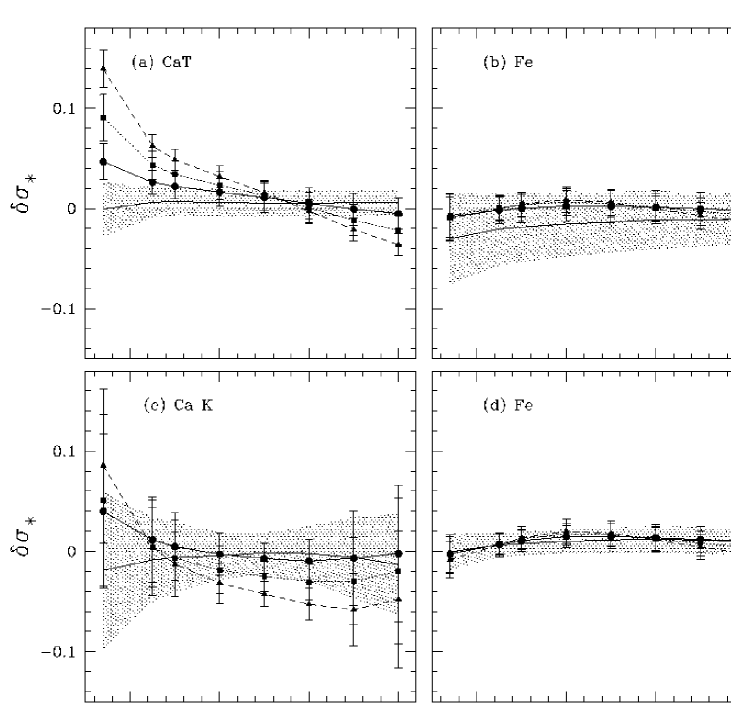
Figure 1: Uncertainty, expressed as a fractional difference $\delta\sigma_{\ast}$$\equiv$ [$\sigma{\mathrm{(out)}}-\sigma{\mathrm{(in)}}$]$/\sigma{\mathrm{(in)}}$, due to template mismatch for (a) CaT, (b) the Fe region (5250–5820 Å), and (c) Ca K. We create 100 different model galaxies from random collections of 10 template stars, and depict one standard deviation above and below the mean $\delta\sigma_{\ast}$ by the shaded region. The mean is demarcated by the thin solid line. We also run simulations with 10% (circles), 20% (squares), and 30% (triangles) A star contribution. The points represent the mean $\delta\sigma_{\ast}$, and the error bars are one standard deviation in $\delta\sigma_{\ast}$. Because of the strange behavior of Fe shown in (b), we present alternate simulations in (d) excluding the six largest outliers.

Many factors may contribute to uncertainties in our $\sigma_{\ast}$ measurements, including template mismatch, resolution, and S/N (we discuss emission from the AGN separately). By generating model spectra, we can examine how each of these factors in turn impacts our ability to recover the input velocity width. We build model galaxies as linear combinations of template spectra, which we then broaden to a range of widths between $\sigma$ = 50 and 400 km s^-1, assuming a Gaussian line-of-sight velocity distribution. We then vary parameters of interest, such as S/N, and evaluate our ability to recover $\sigma_{\ast}$, using as the figure of merit the fractional error $\delta\sigma_{\ast}$ $\equiv$ [$\sigma{\mathrm{(out)}}-\sigma{\mathrm{(in)}}$]/$\sigma{\mathrm{(in)}}$. For later use, we focus on (1) the region around Ca H+K (3910–4060 Å) with Ca H (3955–3985 Å) masked, (2) the region redward of Mg I$b$ (5250–5820 Å; hereafter called the “Fe region”) with [Fe VII] $\lambda 5721$ masked, and (3) the region around the CaT (8470–8700 Å). Each fit is done locally, without attempting to match the polynomial or AGN power-law between regions.

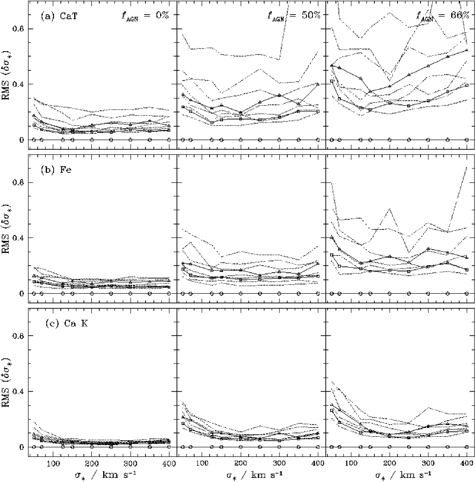
Figure 2: Input-output simulations of velocity dispersion measurements from (a) the CaT region, (b) Fe (5250–5820 Å), and (c) Ca K of galaxy models constructed as the average of 10 template stars. $\delta\sigma_{\ast}$ $\equiv$ [$\sigma{\mathrm{(out)}}-\sigma{\mathrm{(in)}}$]$/\sigma{\mathrm{(in)}}$. Simulations are shown for S/N of 15 to 55, in steps of 5. The highest S/N (i.e., no additional noise) is $\sim$ 205, 240, and 95 for CaT, Fe, and Ca K, respectively (shown in open circles). We highlight in solid lines the cases for S/N = 30 (triangles) and S/N = 50 (squares), since the majority of our data are spanned by these limits. The middle and right columns correspond to $f_{\rm AGN}$ = 50% and 66%, respectively.

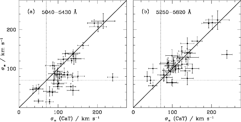
Figure 3: A comparison between $\sigma_{\ast}$ from the CaT region and (a) the Mg Ib region (5040–5430 Å) and (b) the Fe region (5250–5820 Å). Note the large systematic offset at low $\sigma_{\ast}$ in the Mg Ib region. The solid line represents equality, while the dotted lines mark the nominal resolution limit of the SDSS.

To begin with the simplest possible test, we fit a model galaxy, composed of 10 template stars with only artificial broadening, in the CaT region. We are using a single average template in order to increase the effective S/N of our template, but for comparison we also compute $\sigma_{\ast}$ as the average of the values obtained from each of the 32 individual template stars. The resulting $\delta\sigma_{\ast}$ values for both approaches are shown in Figure 3. No apparent offset is introduced by the use of an average template, while the fractional error close to the resolution limit is diminished. In general, while additional uncertainty is introduced below $\sigma_{\ast}$ $\approx 100$ km s^-1 due to resolution, it is only on the order of $\sim 2\%$. We follow previous work (e.g., Bernardi et al. 2003; Heckman et al. 2004) and limit our attention only to velocity dispersions larger than the nominal instrumental resolution of SDSS, which we take to be $\sigma_{\rm inst}=70$ km s^-1.

Even for predominantly old stellar populations (G and K giant stars), template mismatch will introduce feature-dependent uncertainties. To investigate the magnitude of these uncertainties for each fitting region, we generate a family of 100 model galaxies. As above, the model consists of 10 templates, which are selected randomly for each run, and then coadded and artificially broadened. The shaded region in Figure 4 represents one standard deviation around $\delta\sigma_{\ast}$ for the ensemble of 100 trials. Note that the CaT region is well-behaved (Fig. 4a), while the Fe region is, on average, $\sim 2\%$ low (Fig. 4b). However, when we remove the six largest outlying templates from the parent set of 32 and repeat the simulations, the negative offset is removed (Fig. 4d). In the Ca H+K region $\delta\sigma_{\ast}$ has a mean value of zero, but by far the largest dispersion.

While this experiment gives us a feel for template mismatch among old stellar populations, additional uncertainty is introduced by young stellar populations. Particularly, it has been shown that the host galaxies of luminous AGNs do not contain a uniformly old population, but rather are more likely to contain a post-starburst population than quiescent galaxies of similar total stellar mass (e.g., Terlevich et al. 1990; Kauffmann et al. 2003b; Nelson et al. 2004). Due to rotational and pressure broadening, a significant A star population can significantly broaden the hydrogen lines, and potentially bias the measurements in the regions around CaT and Ca H+K. Therefore, we run an additional set of simulations in which we explicitly include an A star contribution, using an A star spectrum observed by SDSS, Gaussian-broadened to the same width. In Figure 1 (bottom panel) we show that the A star spectrum has significant features in both the Ca H+K and CaT regions, while it is nearly featureless in the Fe region. In the case of CaT, the features are a blend of Paschen and CaT lines, while the Ca K line is apparent to the left of a blend of Ca H and H$\epsilon$ in the Ca H+K region. The $\delta\sigma_{\ast}$ values for models including A star contributions of 10%, 20%, and 30% are shown in Figure 4. As expected, both the Ca H+K and CaT regions are more sensitive to the presence of A stars, although the impact is relatively small ($\leq 10\%$). Note, however, that the induced spread is largest in the case of Ca H+K.

The situation is more puzzling in the case of the Fe region, where the uncertainties appear to decrease with the addition of an A star component. Apparently an A star contribution leads to a better fit of the outlying templates, which were removed to generate Figure 4d. Various scenarios may account for this behavior. If, for instance, the outliers have a continuum shape opposite to that of an A star (i.e., very red), then the addition of an A star would cancel them out. We investigated this possibility by running simulations including the A star but excluding the outlying templates, shown as points in Figure 4d, but the induced errors do not increase, so this is probably not the solution. Another possibility is that the outlying templates have stellar absorption features with larger EWs, so that the additional dilution from the A star continuum improves their fit with the rest of the templates. We measured the EW in Mg I$b$ (using the Lick index definition; e.g., Trager et al. 1998) for each individual template, and the mean EW for the outliers is 5.2 Å, compared to $\langle$EW$\rangle$ = 3.3 Å for the rest, indicating this is the most likely explanation. Since our actual galaxies will probably contain some A star contribution, we have decided to retain all 32 templates in our average template, despite the apparent skewness of Figure 4b. We verified that our actual fits are not strongly affected if we use an average template excluding the six outliers. Between the nominal results and those derived from an average template excluding the six outliers, we find an average relative difference of $\langle$$\delta\sigma_{\ast}$$\rangle=-0.06\pm 0.1$.

We now turn to the impact of varying S/N on the reliability of our measurements. For these simulations, we begin with a well-behaved model galaxy from the simulation above. We degrade the S/N by adding mean-zero Gaussian random deviates, whose uncertainty at each pixel is given by the SDSS pipeline error array, and whose amplitude is varied to decrease the effective S/N from 60 to 15, in steps of 5. Note that the model galaxy has a S/N of $\sim$ 205, 240, and 95 for the CaT, Fe, and Ca H+K regions, respectively, which forms the upper limit on our noise simulations. In practice, the majority of our objects are found between a S/N of 30 and 50 (although the distribution is somewhat lower in the Ca H+K region). For each S/N, we generate 50 model spectra, in order to average over the variations caused, for instance, when a noise spike falls on a crucial absorption feature. We do not find a systematic bias in $\delta\sigma_{\ast}$ from variations in S/N or dilution and so for simplicity we report the standard deviation in $\delta\sigma_{\ast}$over the 50 trials, denoted RMS($\delta\sigma_{\ast}$). The results are shown in the left-hand panels of Figure 5, for each spectral region of interest. From these simulations it is clear that even at the modest S/N of 20, which is common for SDSS spectra, it is possible to achieve $\sigma_{\ast}$ measurements with $\sim 20\%$ accuracy.

4 Measuring $\sigma_{\ast}$ in AGNs

Inspired recently by the discovery of the $M_{\mathrm{BH}}-\sigma_{\ast}$ relation, many groups have measured $\sigma_{\ast}$ in Type 1 AGNs (e.g., Jiménez-Benito et al. 2000; Ferrarese et al. 2001; Barth et al. 2002b, 2003, 2005; Nelson et al. 2004; Onken et al. 2004; Treu et al. 2004; Woo et al. 2004; Botte et al. 2005; Garcia-Rissmann et al. 2005). As noted by many of these authors, measuring $\sigma_{\ast}$ in the presence of an AGN is particularly challenging. The AGN power-law continuum dilutes the stellar features, effectively lowering the S/N, while emission lines from the AGN can add (sometimes subtle) biases into the fits. In order to mitigate these problems, the above studies fit specific spectral regions with minimal AGN contamination but high-EW stellar absorption features, rather than attempting to find global solutions for large regions of the spectrum. We adopt the same approach. In particular, the utility of the CaT region has long been recognized (Pritchet 1978; Dressler 1984). The CaT lines are intrinsically narrow compared to galactic velocity dispersions, with intrinsic widths of $\sigma\approx 20-25$ km s^-1 for K giant stars, ranging up to $\sim 30$ km s^-1 for supergiant stars (Filippenko & Ho 2003; Martini & Ho 2004). Furthermore, the AGN continuum is minimized in their vicinity, since AGN continua are typically blue. Although higher-order Paschen lines (P13 $\lambda 8503$, P15 $\lambda 8545$, and P16 $\lambda 8665$) overlap with the CaT lines, these features are rarely seen in emission (an exception is NGC 4395, which, as noted by Filippenko & Ho, has anomalously high-EW emission features). Emission from CaT itself can fill in the absorption features as well, but these objects were eliminated by selection. Finally, there may also be O I $\lambda 8446$ or [Fe II] $\lambda 8616$ emission from the AGN. In principle we can mask either of these features in a straightforward manner within our fit, but again, these lines are weak by selection in our sample. We measured meaningful $\sigma_{\ast}$ measurements for all but one of our objects, although an additional four are below our nominal resolution limit of $\sim 70$ km s^-1 (Table 1). At the S/N of the SDSS data, our ability to recover accurate $\sigma_{\ast}$ measurements below the resolution limit is significantly decreased, and so we conservatively do not include these four measurements in our analysis.

Of all high-EW features in the optical bandpass, the CaT lines are simultaneously the least affected by template mismatch and AGN contamination, making them our “gold standard.” Unfortunately, because they occur in the red region of the spectrum, they are inaccessible to optical bandpasses above $z\approx 0.05$. For this reason, we must examine the utility of other spectral regions with reasonably strong absorption features. We will focus on two: the region surrounding the Mg I$b$ triplet (5040–5820 Å) and the region around the Ca H+K lines (3900–4060 Å). We measure $\sigma_{\ast}$ using these alternate spectral regions, and compare the results directly with the CaT values. In order to evaluate whether a given test region matches CaT, we use the same figure of merit as defined above, $\delta\sigma_{\ast}$ $\equiv$ [$\sigma{\mathrm{(test)}}-\sigma{\mathrm{(CaT)}}$]/$\sigma{\mathrm{(CaT)}}$, using in all cases the 35 measurements with $\sigma_{\ast}$(CaT) $\geq 70$ km s^-1.

4.1 Power-law Continuum Contamination

Relatively speaking, it is straightforward to model the contaminating effect of a pure power-law component on the final $\sigma_{\ast}$ measurement. We perform simulations identical to those described in §3.2.2, starting with a model composed of 10 template stars, adjusting the S/N from 15 to 60, in steps of 5, and measuring $\delta\sigma_{\ast}$, except that now we also include a power-law component to represent the AGN continuum. We use a single power law, $f_{\nu}\propto\nu^{-1}$, comprising 0, 33, 50, 60, 66, 70, 75, 80% of the total local continuum, as measured in the 20 Å at each end of the band. Assuming our nominal power-law slope of $-1$, an AGN fraction of $50\%$ ($66\%$) in the Fe region corresponds to

Examples of the Mg Ib spectral region for objects with significant Fe II contamination, as well as, in some cases, contamination from [Fe VII]$~{}\lambda 5158$, [Fe VI] $\lambda 5176$, [N I] $\lambda\lambda$5197, 5177, [Fe VII]$~{}\lambda 5278$, [Fe XIV]$~{}\lambda 5303$, and [Fe VI]$~{}\lambda 5335$. Plotted in order of decreasing [Fe VII] strength, from top to bottom, are SDSS J162012.75+400906.1, J120114.35$-$034041.0, J083949.65+484701.4, J112536.16+542257.1, J150745.00+512710.2, and J101912.56+635802.6.

$48\%$ ($65\%$) AGN fraction in the CaT region and $73\%$ ($84\%$) AGN fraction in the Ca H+K region. For general comparison with the literature, we also compute the EW in Mg I$b$, CaT, and Ca H+K from the average template star for AGN fractions of $0\%,50\%$, and $66\%$ in the Fe region. We use the Lick index definition of the Mg I$b$ index (Trager et al. 1998), the Terlevich et al. (1989) definition of the CaT $\lambda 8542$ Å line, and the Brodie & Hanes (1996) definition of the HK index. For no dilution we find EW = 4, 3, and 22 Å for Mg I$b$, CaT, and Ca H+K, respectively. These decrease to EW = 2, 1, and 6 Å for $f_{\rm AGN}$ = 50%, and to EW = 1, 0.9, and 4 Å for $f_{\rm AGN}$ = 66%. We show representative cases with 50% and 66% contamination in the middle and right panels of Figure 5. Although we have run a larger suite of simulations, these examples bracket the majority of the measured values for our sample. We assign an uncertainty to each of our galaxies by interpolating between the grid points from the simulations to its measured S/N and dilution. These simulations show that if template mismatch and AGN emission features were not present, we would achieve the best measurements using the line with the highest EW (namely Ca H+K in this case). While not directly relevant to this particular sample, it is of general interest to determine the limiting AGN dilution for each spectral feature. As a general indicator, we set the maximum AGN dilution at the point where $\delta\sigma_{\ast}$ = 1 at a S/N = 20. This occurs at an AGN fraction of 71% for CaT, 85% for the Fe region, and 90% for Ca H+K. Although the Ca H+K lines endure the highest AGN contamination, they are very susceptible to systematic uncertainties induced by template mismatch, and so we prefer the CaT lines despite their lower EWs.

As a sanity check, we compare to the BL Lac objects studied by Barth et al. (2003), whose dominant sources of uncertainty are S/N and dilution from a pure power-law continuum. For their sample, with dilutions of 50%–80% and S/N between 50 and 300, they find $\sim$2%–11% errors using either the CaT or Mg I$b$ spectral regions. Reassuringly, to the extent that they overlap, our simulations are consistent with their results.

4.2 Emission-line Contamination

As we have seen, contamination from a power-law continuum only effectively lowers the S/N of the measurement. Far more pernicious are the subtle biases that may be introduced by AGN emission features and template mismatch. Between the Mg I$b$ lines themselves and the prominent Fe I blends at 5270 Å and 5335 Å, this region contains sufficiently high-EW features for measuring velocity dispersion, but they are susceptible to template mismatch due to metallicity effects. Because of the well-known correlation between [Mg/Fe] and $\sigma_{\ast}$ (e.g., O’Connell 1976; Worthey et al. 1992; Trager et al. 1998; Jørgensen 1999; Kuntschner et al. 2001), it becomes increasingly difficult to simultaneously fit both the Mg I$b$ and Fe features using template spectra with solar metallicities and abundance ratios. The errors incurred are small, but increase with increasing $\sigma_{\ast}$, tending to artificially increase the inferred velocity dispersion (Barth et al. 2002a).

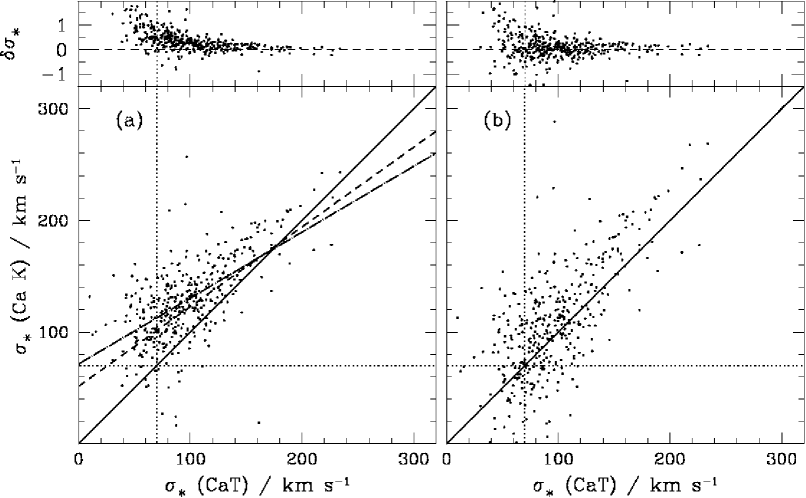
Figure 6: (a) Velocity dispersion measurements for a sample of 374 Type 2 Seyfert galaxies from Heckman et al. (2004), with $z<0.03$ and S/N $>10$ in the CaT region. We have measured $\sigma_{\ast}$ using both the CaT and the Ca K regions. The solid line denotes $\sigma$(Ca K) = $\sigma$(CaT); the dashed line shows the fit derived from Figure 11 for an alternate set of Seyfert 2 galaxies (Eq. 2; see text for details), the dash-dot line shows the fit derived for this sample (Eq. 3), and the dotted lines mark the SDSS resolution limit. $\langle\mathrm{[}\sigma{\mathrm{(Ca~{}K)}}-\sigma{\mathrm{(CaT)}}\mathrm{]}/\sigma{\mathrm{(CaT)}}\rangle=0.29\pm 0.29$ km s^-1. (b) The same as (a), except that we have corrected the Ca K values using Equation 2, shown in (a) as a dashed line. We denote equality of the two velocity dispersion measures with a solid line. After the correction, $\langle\mathrm{[}\sigma{\mathrm{(Ca~{}K)}}-\sigma{\mathrm{(CaT)}}\mathrm{]}/\sigma{\mathrm{(CaT)}}\rangle=0.11\pm 0.34$ km s^-1.

Perhaps more relevant to this study, there is significant AGN line contamination over this wavelength range. There are a number of narrow emission lines, including [Fe VII]$~{}\lambda 5158$, [Fe VI] $\lambda 5176$, [N I] $\lambda\lambda$5197, 5200, [Fe VII]$~{}\lambda 5278$, [Fe XIV]$~{}\lambda 5303$, and [Fe VI]$~{}\lambda 5335$ (see Fig. 6). The first three lines are especially troublesome, occurring as they do amidst the Mg I$b$ features, and they are present in $\sim 50\%$ of our sample. In addition to narrow features, there is a broad Fe II “pseudo-continuum,” extending from $\sim$5050 to 5520 Å (e.g., Francis et al. 1991). When the Fe II emission is broad enough to be smooth, it simply lowers the effective S/N of the spectrum without introducing significant systematic errors (e.g., Nelson & Whittle 1995). However, when the broad-line velocity is low enough that the individual Fe II components are relatively resolved, then the resulting $\sigma_{\ast}$ measurements may be biased. Some examples of galaxies with significant broad Fe II contamination as well as strong coronal emission lines are shown in Figure 6.

Following Barth et al. (2002a), we use the region extending 5040 to 5430 Å, and we mask the [N I] feature from 5190–5210 Å. In Figure 7a, we compare the velocity dispersions obtained from this fit with those from CaT. As is immediately clear, $\sigma$(Mg I$b$) is significantly biased. In particular, there is a plume of objects with $\sigma{\mathrm{(CaT)}}$ values between 75 and 150 km s^-1 and $\sigma{\mathrm{(Mg{\tiny I}{\it b})}}\approx 80$ km s^-1. We find $\delta\sigma_{\ast}$ = $\langle\mathrm{[}\sigma{\mathrm{(Mg{\tiny I}{\it b})}}-\sigma{\mathrm{(CaT)}}\mathrm{]}/\sigma{\mathrm{(CaT)}}\rangle$ = $-$0.23 $\pm$ 0.32. A combination of broad, permitted Fe II emission and high-ionization forbidden emission must be responsible for this dramatic offset, since mismatches in [Mg/Fe] tend to go in the opposite direction. We use simulations to gauge the systematic effects due to Fe II contamination, and we experiment with different spectral regions to minimize the effects of coronal emission.

We examine the role of broad Fe II contamination by running simulations, similar to those presented in §3.2.2. In the usual way, we create a model galaxy using 10 of our template stars and Gaussian-broaden it artificially to widths between 50 and 400 km s^-1. As a model of the Fe II contamination we utilize the Fe II spectrum of I Zw 1 (Boroson & Green 1992), kindly provided by T. A. Boroson. I Zw 1 is a narrow-line Seyfert 1 galaxy, which for our purposes ensures that the Fe II emission is both strong and narrower than the Fe II emission in our objects. The challenge is simulating a representative range of EWs and velocity dispersions for the Fe II template that accurately reflect what is found in real AGNs. In the sources of interest the Mg I$b$ features are strong (and thus measurable), making it difficult to accurately determine the Fe II EW, at least in a model-independent way. We have chosen to vary the Fe II amplitude between an EW of 18 and 54 Å, comparable to what is seen in relatively weak Fe II emitters. For instance, Boroson & Green (1992) find a range of Fe II EWs between 0 and 114 Å for their sample of nearby quasars. As demonstrated in Figure 8, this level of Fe II contamination is hard to discern based on the appearance of the absorption features. However, despite the low amplitude, this quantity of Fe II contamination can seriously bias the fits. Far more important than the amplitude of contamination is the width of the Fe II lines. When they are narrow enough to have significant structure, they most effectively confuse the fitting procedure. Empirically, the width of the Fe II emission is found to match that of the broad component of H$\beta$ (e.g., Boroson & Green 1992). Therefore, using the $M_{\mathrm{BH}}-\sigma_{\ast}$ relation, for any given $\sigma_{\ast}$ the range of possible Fe II widths is set by the luminosity of the AGN through the line width-luminosity relation ($M_{\mathrm{BH}}$ $\propto$ $L^{0.64}$$\mathrm{FWHM}_{\mathrm{H{\beta}}}$²; Kaspi et al. 2005; Greene & Ho 2005b). Since, for a given $M_{\mathrm{BH}}$ the maximum luminosity is set by the Eddington limit, it is convenient to parameterize the AGN luminosity using the Eddington ratio, $L_{\mathrm{bol}}/L{\mathrm{{}_{Edd}}}$, where $L_{\mathrm{Edd}}\equiv 1.26\times 10^{38}$ ($M_{\mathrm{BH}}$/$M_{\odot}$) ergs s^-1. In practice, the bolometric luminosity is difficult to obtain, and so we assume a canonical bolometric correction of 0.1 between the optical and bolometric luminosities (e.g., Elvis et al. 1994). For a fixed $\sigma_{\ast}$ (or equivalently $M_{\mathrm{BH}}$), as the luminosity of the system increases the line width must decrease, such that the narrowest Fe II lines are found at the highest $L_{\mathrm{bol}}/L{\mathrm{{}_{Edd}}}$. Hence, the worst contamination occurs at the Eddington limit, as shown in Figure 9, where we consider $L_{\mathrm{bol}}/L{\mathrm{{}_{Edd}}}$ = 0.01, 0.1, and 1. Also, for any given value of $L_{\mathrm{bol}}/L{\mathrm{{}_{Edd}}}$, the bias is worst near the resolution limit. We do not show the simulations with Fe II EW of 18 or 54 Å, but the general trends are the same, with a maximum bias in the Mg I$b$ region of $\sim 10\%$ for an EW of 18 Å and $\sim 30\%$ for an EW of 54 Å. In addition to the 5040–5430 Å region, we also consider the region 5250–5820 Å, which eliminates the Mg I$b$ features themselves but includes the Fe I absorption features. As we will show below, this is a better spectral region to use in cases with strong [N I] and coronal emission from [Fe VII]. We find that this spectral region is somewhat better behaved at low $\sigma_{\ast}$ and low Eddington ratio, but worse at large $\sigma_{\ast}$ and at high $L_{\mathrm{bol}}/L{\mathrm{{}_{Edd}}}$ (Fig. 9b). Finally, we consider the effects of Fe II contamination on the Ca H+K lines. The Fe II features near $\sim 3950$ Å are both weaker and broader (see bottom of Fig. 1), which means that the maximum incurred bias is $\leq 20\%$ (Fig. 9c; $\sim 10\%$ for EW of 18 Å and $\sim 30\%$ for an EW of 54 Å), except near the resolution limit. We note that while we have run a suite of simulations including many combinations of $L_{\mathrm{bol}}/L{\mathrm{{}_{Edd}}}$ and EW, in nature the Fe II strength is found to increase with $L_{\mathrm{bol}}/L{\mathrm{{}_{Edd}}}$ (e.g., Boroson 2002), further contaminating sources close to their Eddington limit.

Given the rather large bias that Fe II emission can apparently cause, especially at high Eddington ratios, we seek a general method to salvage the Mg I$b$ region by including an Fe II model directly in our direct-fitting code. Equation 1, describing our fitting procedure, includes a term $C(x)$, which is a model of the AGN continuum. Previously we have modeled the AGN component as a pure power law, but now we also include the I Zw 1

Examples of simulations including Fe II contamination. The stellar continuum is modeled as the average of 10 template stars, while the Fe II contamination is modeled using the Fe II template derived from I Zw 1. The template is scaled to Fe II EWs of 18, 36, and 54 Å in our models, while the line width is parameterized using the Eddington ratio ($L_{\mathrm{bol}}/L{\mathrm{{}_{Edd}}}$; see discussion in text). From top to bottom we illustrate $L_{\mathrm{bol}}/L{\mathrm{{}_{Edd}}}$ = 0.01, 0.1, and 1 with EW(Fe II) = 36 Å, and $L_{\mathrm{bol}}/L{\mathrm{{}_{Edd}}}$ = 1 with EW(Fe II) = 54 Å. The bottom spectrum represents the most extreme contamination examined in our simulations. Note that in all cases the effects of the Fe II on the stellar features are subtle (for instance, there is a change in the relative strengths of the Mg Ib triplet).

Figure 4: The effect of Fe II contamination on $\sigma_{\ast}$. We compare the systematic offsets introduced in three different spectral regions: (a) Mg Ib, (b) the Fe region redward of Mg Ib, and (c) Ca K. The model spectrum used in the simulations is the average of 10 template stars, with Fe II contamination added using the I Zw 1 template. The amplitude of Fe II is kept constant for these simulations with an EW of 36 Å, but its velocity width decreases as the Eddington ratio increases. We use the input $\sigma_{\ast}$ value to calculate $M_{\mathrm{BH}}$, and the assumed $L_{\mathrm{bol}}/L{\mathrm{{}_{Edd}}}$ value sets the continuum luminosity. We then infer FWHM of H$\beta$, which empirically matches the FWHM of Fe II (e.g., Boroson & Green 1992). The percentage systematic error introduced is quantified by $\delta\sigma_{\ast}$ $\equiv$ [$\sigma{\mathrm{(out)}}-\sigma{\mathrm{(in)}}$]$/\sigma{\mathrm{(in)}}$.

Fe II template. In so doing we introduce three new degrees of freedom: a velocity shift, a velocity dispersion, and an amplitude for the Fe II spectrum. Rather than allowing these parameters to vary freely, we adopt an iterative process. Initially we perform the standard fit as described above with no Fe II component. When Fe II contamination is present, the residuals of the initial fit contain significant Fe II features. We perform a least-squares fit between the residuals and the I Zw 1 template to measure the velocity shift of Fe II, using the region from 5040 to 5820 Å to improve the leverage on the velocity. The shift is then constrained to this value in the final fit, while the Fe II width is fixed to the velocity dispersion of H$\beta$ (when we allow this parameter to be free, the code often fails). In simulations in which we artificially add Fe II contamination and then use this multi-step fitting procedure to remove it, we find that we are able to recover the input $\sigma_{\ast}$ values, with a slight negative offset of $\delta\sigma_{\ast}$$\approx-5\%$, for both spectral regions. This, however, assumes that we know the width of the Fe II lines perfectly. Once we introduce a $20\%$ variation in the Fe II width, the output dispersions have associated errors of $\sim 10\%$.

On the other hand, when we attempt to use this fitting procedure with our actual data, the results are not very encouraging. A slight positive systematic difference of 2%–5% is introduced between the fits with and without the Fe II modeling. As we have noted, our objects are not high-$L_{\mathrm{bol}}/L{\mathrm{{}_{Edd}}}$ objects. Recall that we selected objects with both high CaT absorption EWs and neglible CaT emission. Since CaT emission is correlated with Fe II emission, which in turn is correlated with $L_{\mathrm{bol}}/L{\mathrm{{}_{Edd}}}$ (Persson 1988; Persson & Ferland 1989; Boroson 2002), we have predominantly selected AGNs with low Fe II EW and low $L_{\mathrm{bol}}/L{\mathrm{{}_{Edd}}}$. Using virial mass estimates based on H$\alpha$ line width and luminosity (Greene & Ho 2005b), we find $\langle$log $L_{\mathrm{bol}}/L{\mathrm{{}_{Edd}}}$$\rangle=-1.3\pm 0.4$ for this sample (Greene & Ho 2005c). In this regime, when the Fe II emission is very smooth, it is somewhat degenerate with the polynomial in the fit. While the Fe II EW estimates from the code range from 1–300 Å, with a median value of 80 Å, we do not believe these values are well-constrained. It is possible that in more extreme cases, in which the Fe II emission is more pronounced, it may be possible to obtain a more robust fit for the Fe II emission, and thus recover $\sigma_{\ast}$. Of course, high-resolution and high-S/N observations would also aid significantly in performing this procedure.

We conclude that, while broad Fe II contamination can cause large biases in Mg I$b$ measurements, it is not responsible for the offsets observed in Figure 7a between Mg I$b$ and CaT. Instead, narrow coronal emission is probably the primary culprit, which suggests that alternate spectral regions with less coronal emission contamination and, ideally, less Fe II emission as well, need to be explored. The optical Fe II multiplets become negligible at $\sim 5520$ Å, and the region redward of Mg I$b$ is rich in metal lines, which, while having lower EWs, in principle may be used to measure $\sigma_{\ast}$. We have experimented with the following spectral regions: 5520–5820 Å and 5520–6280 Å, which avoid Fe II contamination almost completely, as well as both 5040–5820 Å and 5040–6280 Å. Finally, we tried a compromise region, 5250–5820 Å, which contains the high-EW Fe I absorption features, at the expense of some Fe II contamination. In all cases, we mask 5710–5740 Å to remove the often-present [Fe VII] $\lambda 5721$ line, and, where relevant, we mask 5820–5950 Å to exclude the Na D feature, which is susceptible to strong interstellar contamination (e.g., Bica et al. 1991). In cases including the Mg I$b$ and Fe II features we have experimented with masking the Mg I$b$ features themselves, as well as other regions most contaminated by Fe II emission (specifically 5250–5325 Å). We have found that including the spectral region redward of Na D introduces significant template mismatch problems, and therefore do not consider it further. Of all the possibilities remaining, we find that the region 5250–5820 Å minimizes the systematic offset with CaT (as shown in Fig. 7b). With $\langle$$\delta\sigma_{\ast}$$\rangle$ = $\langle\mathrm{[}\sigma{\mathrm{(Fe)}}-\sigma{\mathrm{(CaT)}}\mathrm{]}/\sigma{\mathrm{(CaT)}}\rangle$ = $-0.018\pm$ 0.20, this region is unambiguously superior to Mg I$b$ both in terms of systematic offset and total scatter. Because narrow coronal emission is common and introduces a strong systematic uncertainty, we recommend using the Fe region rather than the Mg I$b$ region itself. However, we note that, at least with the moderate resolution and S/N of SDSS data, it is preferable to avoid both the Fe and Mg I$b$ regions when either the AGN fraction is $\mathrel{\hbox{\hbox to0.0pt{\hbox{\lower 4.0pt\hbox{$\sim$}}\hss}\hbox{$>$}}}$85% or $L_{\mathrm{bol}}/L{\mathrm{{}_{Edd}}}$ $\approx 1$.

4.3 Ca H+K

The Ca H+K lines are also high-EW spectral features potentially useful for obtaining $\sigma_{\ast}$ measurements. Traditionally they have been avoided for a variety of reasons. Perhaps the most serious complication is that their line shapes are a strong function of spectral type, causing systematic errors from template mismatch (e.g., Kormendy & Illingworth 1982; Kobulnicky & Gebhardt 2000). Since H$\epsilon$ overlaps with Ca H and H8 sits directly blueward of Ca K, young stellar populations may seriously affect the region (e.g., Gebhardt et al. 2003). Apart from line shape, there is a very steep gradient in the local continuum (the “4000 Å break”) whose slope depends on spectral type. An additional problem is caused by possible interstellar absorption in the host galaxy, which would lead to narrow cores (see top panel in Fig. 1). Finally, the lines have limited utility at low $\sigma_{\ast}$ because they are, relatively speaking, intrinsically broad. In combination, these factors cause the Ca H+K lines to systematically overestimate $\sigma_{\ast}$, as found by both Kormendy & Illingworth (1982) and Bernardi et al. (2003). Dressler (1979), on the other hand, finds no systematic offsets between the Ca H+K region and the G-band (itself sensitive to template mismatch). However, Dressler was observing a cD galaxy, which, due to the (presumably exclusively) old stellar population and large velocity dispersion ($>375$ km s^-1) offers the most favorable conditions for using Ca H+K. For a sample of late-type galaxies, Kobulnicky & Gebhardt (2000) obtain reasonable agreement ($\sim 20\%$) between Ca H+K absorption line widths and kinematics inferred from H I and [O II] $\lambda 3727$ emission line widths. Note, however, that a comparison with emission features is not the same as a direct comparison with stellar absorption features. Also, as emphasized by Kobulnicky & Gebhardt, their success hinges on their ability to include a wide range of spectral types in the modeling.

Of course, AGN contamination only makes the situation more complicated. The power-law continuum is rising steeply to the blue, fractionally increasing the AGN contamination there, and H$\epsilon$ (and in principle [Ne III] $\lambda$3968) emission renders the Ca H line completely unusable. On the positive side, compared to the Mg I$b$ region, as we saw in §4.2, Fe II contamination is relatively minimal. Despite these many complications, Ca H+K presents two major benefits compared to all other spectral regions. First of all, it is the only stellar feature with sufficient EW to persist in high-luminosity AGNs; for instance, it is detected in the composite SDSS quasar spectrum of Vanden Berk et al. (2001). Secondly, the lines are blue enough to remain in the optical bandpass beyond a redshift of 1. Ca H+K represents our only hope of obtaining $\sigma_{\ast}$ measurements in powerful AGNs or those at intermediate redshift. Below we investigate whether, despite its problems, the Ca H+K region can provide a useful diagnostic of $\sigma_{\ast}$ in AGNs.

Figure 5: (a) A comparison of $\sigma_{\ast}$ using the CaT and Ca K spectral regions. The solid line represents perfect agreement, while the dotted lines mark the nominal resolution limit of the SDSS. Error bars are derived as described in §3.2.2. (b) Same as (a), except that we have corrected the Ca K measurements using Equation 2. It is clear that the correction is too large at low $\sigma_{\ast}$.

We follow the approach of the previous section, and compare $\sigma_{\ast}$ from Ca H+K with that from CaT to seek the combination of spectral region, polynomial order, and masking that yields the best agreement. In terms of the best spectral fitting region, we have found that broad H$\epsilon$ emission is always a contaminant of Ca H. Even when the emission line is not clearly visible, the centroid of the Ca H line is clearly displaced from its expected position relative to Ca K, so that the code cannot find a reasonable solution. For that reason, we simply mask the Ca H line (3955–3985 Å) in all fits; hereafter, our discussion will focus exclusively on the Ca K line. Over this very restricted spectral region, AGN dilution can be somewhat degenerate with increasing velocity dispersion. To mitigate this problem, we include 50 Å of continuum redward of Ca H in order to help the code determine the general level of AGN contamination. Because of the limited spectral region, we also experimented with fewer polynomial orders or a power-law continuum constant with wavelength, but in both cases the final $\chi^{2}$ values were elevated, and the fits were unsatisfactory. Finally, we attempted a two-step fitting approach to try to mitigate the potential bias caused by a narrow core from interstellar absorption. The first iteration was as described above, while for the second iteration we masked the line core but simultaneously fixed the velocity shift. Unfortunately, when only the wings are available, the $\sigma_{\ast}$ measurements become extremely (unphysically) broad, so this technique is untenable. In the end, we settled on a fitting region of 3910–4060 Å with Ca H masked. The results of the comparison with CaT are shown in Figure 10. We find $\langle$$\delta\sigma_{\ast}$$\rangle$ = $\langle\mathrm{[}\sigma{\mathrm{(Ca~{}K)}}-\sigma{\mathrm{(CaT)}}\mathrm{]}/\sigma{\mathrm{(CaT)}}\rangle=0.049\pm 0.29$ km s^-1, which is fairly reasonable agreement.

As noted above, the Ca H+K lines have been known to overestimate $\sigma_{\ast}$, even in the absence of AGN contamination. To evaluate the type of systematic errors that may ensue over a larger range of $\sigma_{\ast}$ in the absence of AGN contamination, we measured $\sigma{\mathrm{(Ca~{}K)}}$ for the sample of 504 SDSS Type 2 Seyfert galaxies described in §3.2.1. As can be seen in Figure 11, $\sigma{\mathrm{(Ca~{}K)}}$ is systematically biased, in a $\sigma_{\ast}$-dependent way. At low $\sigma_{\ast}$ the Ca K values are too large, while at large values of $\sigma_{\ast}$ the Ca K values are too small, with the change occurring at $\sigma_{\ast}$ $\approx 175$ km s^-1. Since the comparison for our program objects is between CaT and Ca K, it may be more appropriate to investigate offsets between these two spectral regions. We have therefore compiled an alternate sample of 374 objects from Heckman et al. (2004) that have $z<0.03$ and a S/N $>10$ around the CaT. Unfortunately, because of the redshift constraint, the velocity dispersions of the sample are low ($<225$ km s^-1), and so we cannot investigate global behavior from these points alone, but the qualitative offset is similar to that seen in the large sample (Fig. 12). This trend is somewhat reminiscent of the bias apparent in $\sigma_{\ast}$(Ca H+K) shown in Figure 4c due to an A star component, which suggests that the bias may be due to

Comparison between $\sigma_{\ast}$ from 4000–6200 Å as compared to Ca K, for a sample of 504 Type 2 Seyfert galaxies from Heckman et al. (2004). The solid line represents equality of the two measurements, and the dotted lines mark the nominal SDSS resolution limit of 70 km s^-1. The dashed line shows our linear least-squares fit (Equation 2). The top panel plots the fractional difference $\delta\sigma_{\ast}$$\equiv$ [$\sigma{\mathrm{(Ca~{}K)}}-\sigma{\mathrm{(4000-6200\AA)}}$]$/\sigma{\mathrm{(4000-6200\AA)}}$.

differing A star contaminations as a function of $\sigma_{\ast}$. We investigate whether young stellar populations are responsible for the observed offsets by seeking a correlation between $\delta\sigma_{\ast}$ and the H$\delta$ index tabulated by Brinchmann et al. (2004; Kauffmann et al. 2003a). In the case of the larger sample the correlation, while highly significant, is weak (Kendall’s $\tau=0.22$, $P_{\mathrm{null}}=10^{-5}$), while for the CaT comparison sample the correlation strength is even weaker (Kendall’s $\tau=0.14$, $P_{\mathrm{null}}=5\times 10^{-4}$). The largest values of $\delta\sigma_{\ast}$ correspondingly have the largest H$\delta$ indices, but a large H$\delta$ index does not ensure a large $\delta\sigma_{\ast}$. While young stellar populations apparently do play a role in driving the observed deviations, they may not fully account for it. We have also investigated whether including H$\delta$ as a secondary parameter improves the correlation between $\sigma$(Ca K) and $\sigma$(4000-6200 Å) or $\sigma$(CaT), using the partial Kendall’s $\tau$ test from Akritas & Siebert (1996). In both cases the partial correlation coefficient is lower than the correlation between the two $\sigma_{\ast}$ variables alone. We thus do not have a complete explanation for the offset at this time.

Nevertheless, we can use the trend observed in Figure 11 to derive a correction for the Ca K velocity dispersions. We use an ordinary least-squares fit, and derive the errors using bootstrap simulations. We find

$$\sigma_{\ast}\ =1.40(\pm 0.04)\sigma{\mathrm{(Ca~{}H+K)}}-71(\pm 5).$$ (2)

We also calculate a correction using the CaT comparison sample only:

$$\sigma_{\ast}\ =1.7(\pm 0.1)\sigma{\mathrm{(Ca~{}H+K)}}-121(\pm 13).$$ (3)

The two corrections are not consistent within the estimated uncertainties, but when we apply Equation 2 to the CaT data set, we do significantly improve the agreement between $\sigma$(Ca K) and $\sigma$(CaT). Prior to correction, $\langle$$\delta\sigma_{\ast}$$\rangle$ = $\langle\mathrm{[}\sigma{\mathrm{(Ca~{}K)}}-\sigma{\mathrm{(CaT)}}\mathrm{]}/\sigma{\mathrm{(CaT)}}\rangle$ = $0.29\pm 0.29$. After applying the correction from Equation (2; see Fig. 12b), we find $\langle$$\delta\sigma_{\ast}$$\rangle$ = $0.11\pm 0.34$, while when we use the correction derived from this data set, we find $\langle$$\delta\sigma_{\ast}$$\rangle=0.0015\pm 0.35$. Clearly the correction derived from the CaT data is superior in the sense that the mean difference is closer to zero after the correction is applied. However, it is worth noting that the scatter increases significantly ($\sim 20\%$) in both cases. Although the scatter increases, thus limiting the achievable precision, the most crucial point is that we can control the systematic bias in the case of the Type 2 objects shown here.

Figure 7: Input-output simulations of velocity dispersion measurements from the Ca H+K region, similar to Figure 5, but with higher AGN contamination. Galaxy models constructed as the average of 10 template stars. $\delta\sigma_{\ast}$ $\equiv$ [$\sigma{\mathrm{(out)}}-\sigma{\mathrm{(in)}}$]$/\sigma{\mathrm{(in)}}$. Simulations were carried out for S/N from 15 to 55, in steps of 5. The highest S/N (i.e., no additional noise) is $\sim$ 95 (shown in open circles). As in Figure 5, we highlight in solid lines S/N = 30 (triangles) and S/N = 50 (boxes). We show an AGN component comprising (left) 90% and (right) 98% of the total continuum.

If this is a valid correction, we should be able to apply it to our AGNs, a completely independent sample of objects, and improve their agreement with CaT. We have performed this test in Figure 10b, using Equation 2. In general we are overcorrecting at low $\sigma_{\ast}$, leading to $\langle$$\delta\sigma_{\ast}$$\rangle$ = $-0.15\pm 0.39$ (the scatter and offset become worse when Eq. 3 is employed). To determine whether Type 1 AGNs in general can be treated in this manner will require a larger database of velocity dispersion measurements spanning a wider range in $\sigma_{\ast}$. We are currently assembling just such a sample (J. E. Greene & L. C. Ho, in preparation). While corrections of this nature are very dangerous, depending as they do on the detailed stellar populations of a given sample, we emphasize again that the Ca H+K lines may be the only available stellar features for estimating $\sigma_{\ast}$ in high-luminosity AGNs. To illustrate that the Ca K line can be used even at very high levels of AGN dilution, in Figure 13 we show simulations for AGN continuum fractions of 90% and 98%. As can be seen, even with an AGN fraction as high as 90% the Ca K line can still provide an estimate of $\sigma_{\ast}$ to within a factor of 2, for a moderate S/N of 20. However, with 98% AGN dilution, there is no hope of obtaining a meaningful measurement of $\sigma_{\ast}$.

5 Practical Guidelines

The optimal spectral region for measuring $\sigma_{\ast}$ depends on the Eddington ratio and continuum level of the AGN, as well as the redshift of interest. For $z<0.05$, CaT is the region of choice. In the redshift interval of $0.05<z<0.76$, the Fe region is the best option, provided that the Eddington ratio is $\mathrel{\hbox{\hbox to0.0pt{\hbox{\lower 4.0pt\hbox{$\sim$}}\hss}\hbox{$<$}}}$0.5 and the overall dilution level is $\mathrel{\hbox{\hbox to0.0pt{\hbox{\lower 4.0pt\hbox{$\sim$}}\hss}\hbox{$<$}}}$85%. Otherwise, the Ca K line must be used. Finally, for $0.76<z<1.3$ Ca K is the only available choice (assuming the observations are made in the optical band).

We summarize these findings schematically in Figure 14. For a given $M_{\mathrm{BH}}$, we estimate the bulge luminosity using the relation of Marconi & Hunt (2003), log ($M_{\mathrm{BH}}$/$M_{\odot}$) = $1.26(\pm 0.13$) [log ($L_{B}/L_{\sun}$)$-10$] $-\,2.96(\pm 0.48$). If we make the simplifying assumption that the entire bulge and only the bulge is contributing to the starlight, we can then estimate the AGN dilution in the $B$ band for any AGN luminosity (expressed here in Eddington units). Of course, this is an approximation that is aperture-dependent. At $z=0.1$, the projected SDSS aperture of 5 kpc is well matched to the effective radius $R_{\mathrm{eff}}\approx 4$ kpc of a $\sigma_{\ast}$ = 150 km s^-1 bulge (Bernardi et al. 2003; Greene & Ho 2005a), while at higher $z$ we are more likely underestimating the total contribution from starlight. We further caution that the actual AGN contamination will differ between spectral regions, becoming worse toward the blue (see §4.1). Finally, there is significant intrinsic scatter in the $M_{\mathrm{BH}}$-$L_{\mathrm{bulge}}$ relation; Marconi & Hunt estimate that the intrinsic scatter is 0.48 dex. Using corrections from Fukugita et al. (1995) to convert from $m_{B}$ to $m_{i}$, we further indicate the maximum redshift to which an AGN of $m_{i}=19.1$ mag (the SDSS magnitude limit for AGN-selected spectroscopic selection) would be detected by the SDSS. The lines of constant redshift shift to the right or left for brighter or fainter apparent magnitudes, respectively. Bear in mind that these lines are schematic only. We do not account for the combined (AGN plus host galaxy) color of the system, and it would be more appropriate to apply the SDSS galaxy magnitude limit below a certain AGN fraction. However, our goal here is simply to illustrate how the different constraints define natural regions in the $M_{\mathrm{BH}}$-$f_{\mathrm{AGN}}$ plane.

We have assumed that the observations are limited to optical wavelengths. Although spectroscopy in the near-infrared is challenging, due to telluric absorption features and strong and variable emission from the night sky, it may be the best option in some cases. For instance, narrow-line Seyfert 1 galaxies, thought to be low-mass BHs at high $L_{\mathrm{bol}}/L{\mathrm{{}_{Edd}}}$ (e.g., Pounds et al. 1995; Boller et al. 1996), typically contain such strong Fe II contamination that CaT may be the only measurable absorption line. Of course, the chances of strong Ca II emission are also highest in these objects, making the determination of $\sigma_{\ast}$ particularly challenging (e.g., Botte et al. 2004; Barth et al. 2005).

6 Summary

We present a statistically significant sample of 40 AGNs with measurable velocity dispersion ($\sigma_{\ast}$) using regions surrounding the Ca II triplet, the Mg I$b$ triplet, and Ca H+K lines, for the purposes of intercomparison. Using a newly developed direct-fitting code, we perform a comprehensive set of simulations and

Schematic diagram to delineate the regimes in which the different spectral regions can be most effectively used to measure $\sigma_{\ast}$. The solid curves mark the three key redshift intervals ($z$ = 0.05, 0.76, and 1.3) to which an $m_{i}=19.1$ mag AGN will be spectroscopically targeted by the SDSS, and the dashed curves identify, from bottom to top, $L_{\mathrm{bol}}/L{\mathrm{{}_{Edd}}}$ = 0.01, 0.1, 0.5, and 1. The fraction of light coming from the bulge was estimated using the $M_{\mathrm{BH}}$-$L_{\mathrm{bulge}}$ relation of Marconi & Hunt (2003).

cross-checks to evaluate the merits and limitations of using each spectral region, with the aim of obtaining realistic estimates of the many systematic uncertainties that affect measurements of $\sigma_{\ast}$ in AGNs. We argue that the Ca II triplet is least susceptible to template mismatch and AGN contamination from emission lines, and so provides the most reliable measurements of $\sigma_{\ast}$. We therefore use these lines as a benchmark to test the other spectral regions.

We examine two types of AGN contamination: featureless continuum dilution that effectively lowers the S/N of the absorption features, and emission lines, both narrow and broad, that fill in the stellar absorption lines and bias the line profiles in subtle ways. In terms of dilution, we find that $\sigma_{\ast}$ is measurable for AGN fractions $\mathrel{\hbox{\hbox to0.0pt{\hbox{\lower 4.0pt\hbox{$\sim$}}\hss}\hbox{$<$}}}$71%, $\mathrel{\hbox{\hbox to0.0pt{\hbox{\lower 4.0pt\hbox{$\sim$}}\hss}\hbox{$<$}}}$85%, and $\mathrel{\hbox{\hbox to0.0pt{\hbox{\lower 4.0pt\hbox{$\sim$}}\hss}\hbox{$<$}}}$90% using Ca II triplet, Mg I$b$, and Ca H+K, respectively. As for AGN emission-line contamination, we find that measurements around Mg I$b$ are very sensitive both to broad Fe II emission and narrow emission from [Fe VI], [Fe VII], and [N I]. The narrow lines can be avoided by using the spectral region 5250–5820 Å. Broad Fe II contamination can bias the fits severely when the Fe II width is narrowest. For a given $M_{\mathrm{BH}}$ this will occur at the highest luminosity, and thus is worst when the object radiates at a large fraction of its Eddington luminosity. In such cases, and for the highest levels of AGN dilution, the Ca H+K spectral region (and particularly the Ca K line) is the best remaining option. While there is a systematic offset between $\sigma$(Ca K) and $\sigma_{\ast}$ derived from other spectral regions, in Type 2 AGNs it is well fit by a linear relation that allows us to derive unbiased $\sigma_{\ast}$ estimates from Ca K. Further work is required to ensure that this correction is generally applicable.

As a by-product of this study, we have derived reliable velocity dispersions for 35 Type 1 AGNs, and set out reasonable selection criteria to generate a much larger sample of AGNs with a broader range of $z$, black hole mass, and accretion rates. Such a sample would enable us to examine the $M_{\mathrm{BH}}-\sigma_{\ast}$ relation for active galaxies with true statistical power. We will be able to calibrate virial masses for black holes with unprecedented accuracy, as well as search for second-order trends in the $M_{\mathrm{BH}}-\sigma_{\ast}$ relation with mass, accretion rate, and redshift. Greene & Ho (2005c) present a preliminary investigation of the $M_{\mathrm{BH}}-\sigma_{\ast}$ relation using the sample analyzed in this study.

References

- (1) Abazajian, K., et al. 2005, AJ, 129, 1755
- (2) Akritas, M. G., & Siebert, J. 1996, MNRAS, 278, 919
- (3) Barth, A. J., Greene, J. E., & Ho, L. C. 2005, ApJ, 619, L151
- (4) Barth, A. J., Ho, L. C., & Sargent, W. L. W. 2002a, AJ, 124, 2607
- (5) ——. 2002b, ApJ, 566, L13
- (6) ——. 2003, ApJ, 583, 134
- (7) Bender, R. 1990, A&A, 229, 441
- (8) Bernardi, M., et al. 2003, AJ, 125, 1817
- (9) Bica, E., Pastoriza, M. G., Da Silva, L. A. L., Dottori, H., & Maia, M. 1991, AJ, 102, 1702
- (10) Blandford, R. D., & McKee, C. F. 1982, ApJ, 255, 419
- (11) Boller, T., Brandt, W. N., & Fink, H. 1996, A&A, 305, 53
- (12) Boroson, T. A. 2002, ApJ, 565, 78
- (13) Boroson, T. A., & Green, R. F. 1992, ApJS, 80, 109
- (14) Botte, V., Ciroi, S., Di Mille, F., Rafanelli, P., & Romano, A. 2005, MNRAS, 356, 789
- (15) Brinchmann, J., Charlot, S., Heckman, T. M., Kauffmann G., Tremonti, C., & White, S. D. M. 2004 (astro-ph/0406220)
- (16) Brodie, J. P., & Hanes, D. A. 1986, ApJ, 300, 258
- (17) Burbidge, E. M., Burbidge, G. R., & Fish, R. A. 1961, ApJ, 133, 393
- (18) Dressler, A. 1979, ApJ, 231, 659
- (19) ——. 1984, ApJ, 286, 97
- (20) Elvis, M., et al. 1994, ApJS, 95, 1
- (21) Ferrarese, L., & Merritt, D. 2000, ApJ, 539, L9
- (22) Ferrarese, L., Pogge, R. W., Peterson, B. M., Merritt, D., Wandel, A., & Joseph, C. L. 2001, ApJ, 555, L79
- (23) Filippenko, A. V., & Ho, L. C. 2003, ApJ, 588, L13
- (24) Francis, P. J., Hewett, P. C., Foltz, C. B., Chaffee, F. H., Weymann, R. J., & Morris, S. L. 1991, ApJ, 373, 465
- (25) Fukugita, M., Shimasaku, K., & Ichikawa, T. 1995, PASP, 107, 945
- (26) Garcia-Rissmann, A., Vega, L. R., Asari, N. V., Fernandes, R. C., Schmitt, H., González Delgado, R. M., & Storchi-Bergmann, T. 2005, MNRAS, 359, 765
- (27) Gebhardt, K., et al. 2000a, ApJ, 539, L13
- (28) ——. 2000b, ApJ, 543, L5
- (29) ——. 2003, ApJ, 597, 239
- (30) Greene, J. E., & Ho, L. C. 2004, ApJ, 610, 722
- (31) ——. 2005a, ApJ, 627, 721
- (32) ——. 2005b, ApJ, 630, 122
- (33) ——. 2005c, ApJ, submitted
- (34) Gunn, J. E., et al. 1998, AJ, 116, 3040
- (35) Heckman, T. M., Kauffmann, G., Brinchmann, J., Charlot, S., Tremonti, C., & White, S. D. M. 2004, ApJ, 613, 109
- (36) Ho, L. C. 1999, in Observational Evidence for the Black Holes in the Universe, ed. S. K. Chakrabarti (Dordrecht: Kluwer), 157
- (37) Jiménez-Benito, L., Díaz, A. I., Terlevich, R., & Terlevich, E. 2000, MNRAS, 317, 907
- (38) Jørgensen, I. 1999, MNRAS, 306, 607
- (39) Kaspi, S., Maoz, D., Netzer, H., Peterson, B. M., Vestergaard, M., & Jannuzi, B. T. 2005, ApJ, 629, 61
- (40) Kaspi, S., Smith, P. S., Netzer, H., Maoz, D., Jannuzi, B. T., & Giveon, U. 2000, ApJ, 533, 631
- (41) Kauffmann, G., et al. 2003a, MNRAS, 341, 33
- (42) ——. 2003b, MNRAS, 346, 1055
- (43) Kelson, D. D., Illingworth, G. D., van Dokkum, P. G., & Franx, M. 2000, ApJ, 531, 159
- (44) Kobulnicky, H. A., & Gebhardt, K. 2000, AJ, 119, 1608
- (45) Kormendy, J., & Illingworth, G. 1982, ApJ, 256, 460
- (46) Kormendy, J., & Richstone, D. 1995, ARA&A, 33, 581
- (47) Krolik, J. H. 2001, ApJ, 551, 72
- (48) Kuntschner, H., Lucey, J. R., Smith, R. J., Hudson, M. J., & Davies, R. L. 2001, MNRAS, 323, 615
- (49) Lynden-Bell, D. 1969, Nature, 223, 690
- (50) Magorrian, J., et al. 1998, AJ, 115, 2285
- (51) Marconi, A., & Hunt, L. K. 2003, ApJ, 589, L21
- (52) Martini, P., & Ho, L C. 2004, ApJ, 610, 233
- (53) Marziani, P., Sulentic, J. W., Dultzin-Hacyan, D., Calvani, M., & Moles, M. 1996, ApJS, 104, 37
- (54) McLure, R. J., & Dunlop, J. S. 2001, MNRAS, 327, 199
- (55) Montgomery, K. A., Marschall, L. A., & Janes, K. A. 1993, AJ, 106, 181
- (56) Moultaka, J., Ilovaisky, S. A., Prugniel, P., & Soubiran, C. 2004, PASP, 116, 693
- (57) Nelson, C. H., Green, R. F., Bower, G., Gebhardt, K., & Weistrop, D. 2004, ApJ, 615, 652
- (58) Nelson, C. H., & Whittle, M. 1995, ApJS, 99, 67
- (59) Netzer, H. 1990, in Active Galactic Nuclei, ed. R. D. Blandford, H. Netzer, & L. Woltjer (Berlin: Springer), 137
- (60) O’Connell, R. W. 1976, ApJ, 206, 370
- (61) Onken, C. A., Ferrarese, L., Merritt, D., Peterson, B. M., Pogge, R. A., Vestergaard, M., & Wandel, A. 2004, ApJ, 615, 645
- (62) Persson, S. E. 1988, ApJ, 330, 751
- (63) Persson, S. E., & Ferland, G. J. 1989, in IAU Symp. 134: Active Galactic Nuclei, ed. D. E. Osterbrock & J. S. Miller (Dordrecht: Kluwer), 293
- (64) Peterson, B. M., et al. 2004, ApJ, 613, 682
- (65) Pounds, K. A., Done, C., & Osborne, J. P. 1995, MNRAS, 277, L5
- (66) Pritchet, C. 1978, ApJ, 221, 507
- (67) Rix, H.-R., Kennicutt, R. C., Jr., Braun, R., & Walterbos, R. A. M. 1995, ApJ, 438, 155
- (68) Rix, H.-W., & White, S. D. M. 1992, MNRAS, 254, 389
- (69) Robertson, B., Hernquist, L., Cox, T. J., Di Matteo, T., Hopkins, P. F., Martini, P., & Springel, V. 2005, ApJ, submitted (astro-ph/0506038)
- (70) Sargent, W. L. W., Schechter, P. L., Boksenberg, A., & Shortridge, K. 1977, ApJ, 212, 326
- (71) Shields, G. A., Gebhardt, K., Salviander, S., Wills, B. J., Xie, B., Brotherton, M. S., Yuan, J., & Dietrich, M. 2003, ApJ, 583, 124
- (72) Silk, J., & Rees, M. J. 1998, A&A, 331, L1
- (73) Simkin, S. M. 1974, A&A, 31, 129
- (74) Spergel, D. N., et al. 2003, ApJS, 148, 175
- (75) Stoughton, C., et al. 2002, AJ, 123, 485
- (76) Strauss, M. A., et al. 2002, AJ, 124, 1810
- (77) Terlevich, E., Díaz, A. I., & Terlevich, R. 1989, Ap&SS, 157, 15
- (78) ——. 1990, MNRAS, 242, 271
- (79) Tonry, J., & Davis, M. 1979, ApJ, 84, 1511
- (80) Trager, S. C., Worthey, G., Faber, S. M., Burstein, D., & González, J. J. 1998, ApJS, 116, 1
- (81) Tremaine, S., et al. 2002, ApJ, 574, 740
- (82) Treu, T., Malkan, M. A., & Blandford, R. D. 2004, ApJ, 615, L97
- (83) Vanden Berk, D. E., et al. 2001, AJ, 122, 549
- (84) van der Marel, R. P. 1994, ApJ, 270, 271
- (85) Vestergaard, M. 2002, ApJ, 571, 733
- (86) Wandel, A., Peterson, B. M., & Malkan, M. A. 1999, ApJ, 526, 579
- (87) Woo, J., Urry, C. M., Lira, P., van der Marel, R. P., & Maza, J. 2004, ApJ, 617, 903
- (88) Worthey, G., Faber, S. M., & González, J. J. 1992, ApJ, 398, 69
- (89) York, D. G., et al., 2000, AJ, 120, 1579
- (90) Zakamska, N. L., et al. 2003, AJ, 126, 2125