Light-cone anisotropy in 21cm fluctuations during the epoch of reionization

Abstract

The delay in light travel time along the line of sight generates an anisotropy in the power spectrum of 21cm brightness fluctuations from the epoch of reionization. We show that when the fluctuations in the neutral hydrogen fraction become non-linear at the later stages of reionization, the light-cone anisotropy becomes of order unity on scales $\ga 50$ comoving Mpc. During this period the density fluctuations and the associated anisotropy generated by peculiar velocities are negligible in comparison.

1 Introduction

Fluctuations in the 21cm brightness from cosmic hydrogen at redshifts $z\ga 6$ were sourced by the primordial density perturbations from inflation (Loeb & Zaldarriaga, 2004; Barkana & Loeb, 2005a, c) as well as by the radiation from galaxies (Scott & Rees, 1990; Madau et al., 1997; Furlanetto, Zaldarriaga, & Hernquist, 2004; Barkana & Loeb, 2005b). These two different components can be separated based on the angular dependence of the 21cm fluctuation power spectrum which is induced by peculiar velocities (Bharadwaj & Ali, 2004; Barkana & Loeb, 2005a). Uncertainties in the cosmological parameters lead to an additional apparent anisotropy due to the Alcock-Paczyński effect; after accounting for constraints from the cosmic microwave background, this effect can still produce up to a $10\%$ anisotropy which may be identifiable because of its particular angular structure (Nusser, 2005; Barkana, 2006). Several low-frequency arrays that could potentially detect the redshifted 21cm signal are being built around the globe, including the Primeval Structure Telescope (web.phys.cmu.edu/$\sim$past), the Mileura Widefield Array (web.haystack.mit.edu/arrays/MWA), and the Low Frequency Array (http://www.lofar.org).

In this work we examine an additional source of anisotropy in the 21cm power spectrum between the directions parallel and transverse to the line of sight. Previous discussions ignored the delay in light travel time (i.e., the “light-cone” constraint) along the line of sight [but see a rough estimate of the effect at the beginning of reionization in an appendix in McQuinn et al. (2006)]. In particular, although the 21cm power spectrum is expected to be measured through averaging over three-dimensional volumes of finite radial extent, the power spectrum was previously evaluated at a fixed time slice of the universe, ignoring the fact that a fixed observing time implies a varying emission time as a function of distance from the observer. Here we evaluate the amplitude of the anisotropy which is sourced by this delay. This time-delay effect is not related to real causal effects or light-crossing times. Since two points at a given separation are in general seen at different redshifts, the correlation function, averaged over all such points, is affected by the change with time of the statistics of ionization (i.e., the distribution of H II regions and their correlation with the underlying density field).

2 Model

Barkana & Loeb (2004) showed that the biased large-scale fluctuations in the number density of galaxies at high redshift imply that the characteristic bubble radius is determined by correlated groups of galaxies rather than by the bubble sizes of individual galaxies. Furlanetto, Zaldarriaga, & Hernquist (2004) developed a semi-analytic model based on this realization, and used it to predict the distribution of H II bubble sizes around a given point (i.e., the one-point distribution of bubbles). Unfortunately, this model cannot be directly applied to estimating two-point distributions. Upcoming 21cm experiments will only have the sensitivity to probe statistical measures of the 21cm fluctuations and will therefore focus on the three-dimensional power spectrum (or, equivalently, the two-point correlation function). We formulate here an approximate model of the 21cm correlation function in order to estimate the time-delay anisotropy.

Suppose that gas with an overdensity $\delta$ and a neutral fraction $x_{n}$ lies in some direction at a distance corresponding to 21cm absorption at a redshift $z$. Then the resulting 21cm brightness temperature offset relative to the CMB is (Madau et al., 1997)

$$T_{b}=28.8\,(1+\delta)x_{n}\,\left(\frac{\Omega_{b}h}{.033}\right)\left(\frac{\Omega_{m}}{.27}\right)^{-\frac{1}{2}}\left({{1+z}\over{10}}\right)^{1\over 2}\,{\rm mK}\ ,$$ (1)

where we have assumed that the IGM has been heated so that $T_{s}\gg T_{\rm CMB}$, and we have substituted the concordance values (Spergel et al., 2003) for the cosmological parameters $\Omega_{b}$, $h$, and $\Omega_{m}$. In order to calculate the two-point correlation function of the 21cm brightness temperature, we must construct the correlated distribution of $\delta$ and $x_{n}$ at two different points observed at two possibly different redshifts. We first estimate the characteristic bubble radius $R_{\rm ch}$ at each redshift, and calculate the mean ionized fraction of the interior of regions of radius $R_{\rm ch}$ as a function of their mean densities. We then calculate the correlation function at two points by integrating over the joint probability distribution of their overdensities.

We first must estimate the characteristic radius $R_{\rm ch}$ at a redshift $z$, defined so that for a given point $P$, the average number of ionizing sources within $R_{\rm ch}$ typically determines whether $P$ is ionized or not. In estimating $R_{\rm ch}$ we must balance two competing trends. On the one hand, if a large region contains enough sources to fully reionize itself, then it will indeed fully reionize regardless of whether small portions within it contain a low density of galaxies; this simple fact favors larger radii over smaller ones. On the other hand, the $\Lambda$CDM density power spectrum implies that the typical magnitude of density fluctuations decreases with scale, so that large regions are unlikely to have a strong positive fluctuation that will increase the number of galaxies sufficiently for them to fully reionize. Thus, we estimate $R_{\rm ch}$ as the largest radius for which a 1-$\sigma$ density fluctuation results in full reionization of a sphere of this radius.

Towards the end of reionization, this simple estimate of $R_{\rm ch}$ approaches infinity, but Wyithe & Loeb (2004) showed that the bubble radius is limited by the finite light travel time to $\sim 70$ comoving Mpc at redshift $\sim 6$; we generalize their argument and set an upper limit on $R_{\rm ch}$ at any stage of reionization. In general, in order to have a coherent ionized bubble of radius $R_{\rm ch}$, various portions of the bubble, some of which are relatively rich with galaxies and some of which have fewer ionizing sources, must effectively exchange photons between them. There are two important timescales: the typical (i.e., 1-$\sigma$) scatter $t_{\rm scatter}$ in the time when different regions of size $R_{\rm ch}$ reach a given stage of galaxy formation (in terms of a given number density of galaxies); and the light crossing time $t_{\rm light}$ of the radius $R_{\rm ch}$. Now, if $t_{\rm light}>t_{\rm scatter}$ at a given redshift $z$, then such a large region will not constitute a single, coherent bubble; e.g., a low-density portion of this region that has not produced enough photons to reionize itself will indeed not be fully reionized at redshift $z$, since the extra ionizing photons needed from the distant portions of the region will typically have been produced a time $\sim t_{\rm scatter}$ earlier but require a time $\sim t_{\rm light}$ to reach the low-density region. We follow Wyithe & Loeb (2004) in using the extended Press-Schechter model (Bond et al., 1991) to estimate this upper limit on $R_{\rm ch}$.

The progress of reionization depends on the total collapse fraction of gas in galactic halos, $F_{\rm col}$, which is determined by integrating the halo mass function over all halos that host galaxies. We use the halo mass function of Sheth & Tormen (1999) which fits numerical simulations accurately (Jenkins et al., 2001). In order to calculate fluctuations in the gas fraction that resides in galaxies within different regions, we adjust the mean halo distribution based on the prescription of Barkana & Loeb (2004) which fits a broad range of simulations. As gas falls into a dark matter halo, we assume it can fragment into stars only if its virial temperature is above $10^{4}$K, which allows for efficient cooling mediated by atomic transitions. We assume that stars dominate over mini-quasars, as expected at high redshift (Wyithe & Loeb, 2005) [but see Madau et al. (2004)]. The stellar spectrum depends on the initial mass function (IMF) and the metallicity of the stars. We consider two examples. The first is the locally-measured IMF of Scalo (1998) with a metallicity of $1/20$ of the solar value, which we refer to as Pop II stars. The second case, labeled as Pop III stars, consists entirely of zero metallicity $M\ga 100\,M_{\odot}$ stars, as expected for the earliest galaxies (Bromm & Larson, 2004).

If we were to treat each sphere of radius $R_{\rm ch}$ as an isolated region, then the mean ionized fraction in a region of mean perturbation $\bar{\delta}$ would simply be related to the gas fraction in galaxies $F_{\rm col}$:

$$\bar{x}_{i}=\left(1+\frac{N_{\rm ion}}{0.76}\right)F_{\rm col}(z,R_{\rm ch},\bar{\delta})\ ,$$ (2)

where $N_{\rm ion}$ is the overall efficiency of emission of ionizing photons per baryon in galactic halos, the factor of 0.76 converts between hydrogen and baryon number densities, and the (minor) addition of 1 counts the gas in galaxies (which need not be ionized by the photons that escape from galaxies). Note that $N_{\rm ion}$ equals the number of ionizing photons produced per baryon in stars, multiplied by the star formation efficiency $f_{*}$ and by the escape fraction $f_{\rm esc}$ of ionizing photons from halos.

In reality different regions are not independent. The overdense regions produce more ionizing photons than they need to fully reionize themselves, and the extra photons expand into the surrounding lower-density regions. In order to make our model consistent with the total number of ionizing photons produced at each redshift, we increase the $\bar{x}_{i}$ values by the amount necessary to achieve consistency. Now, the leakage of additional photons is expected to depend on the mean $\delta$ of the target region. In particular, the deepest voids are likely to be the farthest distance away from the densest regions. We estimate the relative fractions distributed into different regions as follows. For each $\bar{\delta}$, we assume that the increase in $\bar{x}_{i}$ within a region of that $\bar{\delta}$ is proportional to the chance that such a sphere lies next to a sphere with $\bar{\delta}=\delta_{i}$, where $\delta_{i}$ is a high overdensity representative of those regions that have overproduced ionizing photons. We adopt for $\delta_{i}$ the minimum value of $\bar{\delta}$ needed for a sphere to achieve an $\bar{x}_{i}=1$ on its own, i.e., without the help of surrounding regions. In general, we emphasize that the redistribution of photons has a modest effect within our model, consistent with our selection of $R_{\rm ch}$ in such a way that photons from larger distances are unlikely to play a major role in the statistics of reionization.

When we calculate the correlated ionization states of two points at redshifts $z_{1}$ and $z_{2}$, we assume that the ionization probability of each point is determined by the perturbations $\bar{\delta}$ of the surrounding regions of radius $R_{\rm ch}(z_{1})$ and $R_{\rm ch}(z_{2})$, respectively. However, the 21cm brightness temperature $T_{b}$ is determined not only by the neutral fraction but also by the perturbation $\delta$, which is in general different from the spherically-averaged perturbation $\bar{\delta}$. While $\bar{\delta}$ is determined by large-scale power above the scale of $R_{\rm ch}$, the difference $\delta-\bar{\delta}$ is determined by the additional small-scale power within the bubble. In the spirit of the extended Press-Schechter model (Bond et al., 1991), we assume that $\bar{\delta}$ and $\delta-\bar{\delta}$ are approximately statistically independent. We thus add the portion $\delta-\bar{\delta}$ at each point independently of the values of $\bar{\delta}$ and the neutral fraction $\bar{x}_{\rm n}$ of the two regions, with a correlation function for the small-scale portion of $\delta$ set equal to the total $\xi(r)$ of the density field minus the smoothed $\xi(r)$ that determines the joint statistics of $\bar{\delta}$.

When calculating the correlated ionization states of two points we must carefully interpret the values of $\bar{x}_{n,1}$ and $\bar{x}_{n,2}$ in the regions surrounding the two points as probabilities of having neutral gas. For example, the mean value of $x_{n}^{2}$ at point 1 is not $\bar{x}_{n,1}^{2}$, which it would be if the gas were partially ionized with a neutral fraction of $\bar{x}_{n,1}$, but is instead $\bar{x}_{n,1}$ since the gas has $x_{n}=1$ with probability $\bar{x}_{n,1}$ and $x_{n}=0$ with probability $1-\bar{x}_{n,1}$. Thus, the mean expected value of $x_{n,1}x_{n,2}$ must be calculated as the joint probability that both points are neutral. Given the individual probabilities $\bar{x}_{n,1}$ and $\bar{x}_{n,2}$, there is some probability $p_{\rm same}$ that the two points are ionized within the same bubble. Assuming that their ionization probabilities are independent if they are not within the same bubble, we find that

$$\langle x_{n,1}x_{n,2}\rangle=\bar{x}_{n,1}\bar{x}_{n,2}/(1-p_{\rm same})\ .$$ (3)

Now, in order to estimate $p_{\rm same}$ for two points separated by a comoving distance $r$, we note that if one point is ionized by a bubble of radius $R_{\rm ch}$ then the probability that this (randomly-placed) bubble contains a second point a distance $r$ away is zero if $r>2R_{\rm ch}$ and

$$f(r,R_{\rm ch})=1-\frac{3r}{4R_{\rm ch}^{3}}\left(R_{\rm ch}^{2}-\frac{1}{12}r^{2}\right)$$ (4)

otherwise (Furlanetto, Zaldarriaga, & Hernquist, 2004). This yields two estimates of $p_{\rm same}$, starting from either point, so we take the average as our best estimate:

$$p_{\rm same}\approx\frac{1}{2}\left[(1-x_{n,1})f(r,R_{\rm ch}(z_{1}))+(1-x_{n,2})f(r,R_{\rm ch}(z_{2}))\right]\ ,$$ (5)

with the constraint that $p_{\rm same}$ must not be higher than the separate ionization probabilities of each of the two points.

The two-point correlation function $\xi$ of the 21cm brightness temperature $T_{b}$ is a function of the distance $r$ between the two points and their two redshifts. In order to focus on the anisotropy as a function of the angle $\theta$ between the line of sight and the vector connecting the two points, we parameterize $\xi$ as a function of $r$, $\mu\equiv{\rm cos}\theta$, and the redshift $z$ at the midpoint (in terms of comoving distance) of the two points. We calculate the expectation value

$$\xi=\left\langle\left(T_{b,1}-\bar{T}_{b}(z_{1})\right)\times\left(T_{b,2}-\bar{T}_{b}(z_{2})\right)\right\rangle\ ,$$ (6)

assuming that the mean $\bar{T}_{b}$ at the appropriate redshift has been subtracted from $T_{b}$ at each point. Such a subtraction is expected in future observations since the radio measurements take the Fourier transform of the intensity in the $x$ and $y$ directions, removing any sensitivity to a varying $\bar{T}_{b}(z)$ as long as the line $k_{x}=k_{y}=0$ in Fourier space is avoided. We also assume in our results below that $T_{b}(z_{1})$ has been multiplied by $[(1+z)/(1+z_{1})]^{1/2}$, and similarly for $T_{b}(z_{2})$, in order to avoid any anisotropy due to the simple redshift scaling in equation (1).

We calculate the correlation function explicitly by averaging over the joint normal distribution of the perturbations $\bar{\delta}$ of the regions of radii $R_{\rm ch}(z_{1})$ and $R_{\rm ch}(z_{2})$ surrounding the two points. We also calculate the mean value $\bar{T}_{b}(z)$ at each redshift by averaging the quantity $[(1+\delta)x_{n}]$ over the probability distribution. Note that we do not include peculiar velocity fluctuations here since we focus on the late stages of reionization and show that in this regime the 21cm fluctuations and their anisotropy are dominated by ionization fluctuations.

3 Results

We illustrate our predictions for two cases which both assume atomic cooling, a star formation efficiency $f_{*}=2\%$, and an escape fraction of ionizing photons from halos of $f_{\rm esc}=10\%$; however, our low-$z$ case assumes Pop II stars (§ 2) and achieves complete reionization at redshift 7.35, while our high-$z$ case assumes Pop III stars and completes reionization already at redshift 13.7. Note that the parameter values given here assume that only one ionizing photon per hydrogen atom is needed in order to achieve reionization of the IGM. If we assumed instead that several photons are needed due to recombinations, then this would require an increase in the value of $f_{*}$ by the same factor as the required number of photons per atom. This approximation is fairly accurate as long as the number of times each hydrogen atom must be reionized is roughly the same in different regions. Indeed, the recombination rate is not expected to vary greatly in different large-scale regions, since the fluctuation in the mean density of such regions is small. Recombinations can be included in a future refinement of our model.

Figure 1 shows the two reionization histories, as well as the characteristic radius $R_{\rm ch}$ and the standard deviation of the mean density $\bar{\delta}$ in a sphere of radius $R_{\rm ch}$. At each redshift the probability distribution of $\bar{\delta}$ in the spherical region is a Gaussian with this standard deviation; we have not included non-linear corrections which are particularly important early in reionization when $R_{\rm ch}$ is relatively small. The characteristic bubble radius increases during the epoch of reionization as larger groups of galaxies are able to fully reionize the region containing them. At the later stages of reionization, when the cosmic mean $x_{n}\la 10\%$, $R_{\rm ch}$ is determined by the light travel time of ionizing photons.

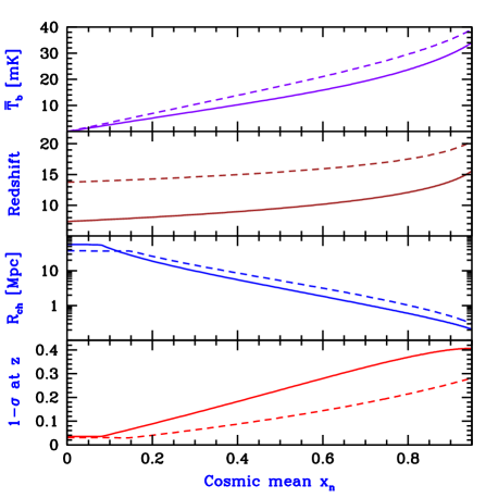
Figure 1: Reionization history. We show the cosmic mean 21cm brightness temperature (top panel), redshift $z$ (next lower panel), the comoving characteristic radius $R_{\rm ch}$ (next lower panel), and the 1-$\sigma$ density fluctuation in spheres of radius $R_{\rm ch}$ at $z$ (bottom panel), each vs. the cosmic mean neutral fraction $x_{n}$. Each panel shows our low-$z$ case (solid curve) and our high-$z$ case (dashed curve).

In Figure 2 we illustrate the correlation function $\xi$ of 21cm brightness temperature late in reionization in the high-$z$ case. If we considered density fluctuations alone (along with a uniform $x_{n}(z)$ equal to its cosmic mean value at each redshift), then $\xi(r)$ would roughly equal the 1-$\sigma$ density fluctuation on scale $r$, times the cosmic mean $T_{b}$, all squared. The growth factor and $x_{n}(z)$ both evolve slowly at this stage of reionization and produce a negligible anisotropy. Adding in peculiar velocities generates a significant anisotropy, but only causes fluctuations that are of order the density fluctuations. However, the ionization fluctuations are far larger and indeed non-linear, since while the bubble radius $R_{\rm ch}$ is large and the corresponding density fluctuations are small (see Figure 1), various regions can have values of $x_{n}$ covering almost the entire possible range of 0–1. In particular, we find that although the 1-$\sigma$ density fluctuation on the scale of $R_{\rm ch}\sim 20$ Mpc is $\sim 0.05$ at this redshift, a negative 2-$\sigma$ void on this scale has an $x_{n}\sim 60\%$ (compared to a cosmic mean $x_{n}$ of $25\%$), while a positive 1-$\sigma$ overdense region is almost completely reionized.

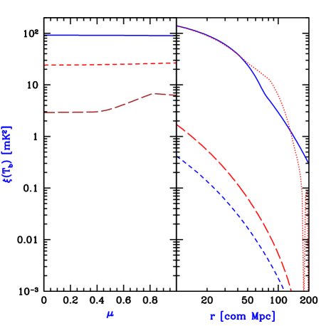
Figure 2: Correlation function of 21cm brightness temperature as a function of $r$ or $\mu$, at a late stage of reionization ($\bar{x}_{n}=0.25$) by Pop III stars. The left panel considers comoving $r=20$ Mpc (solid curve), 50 Mpc (short-dashed curve), and 100 Mpc (long-dashed curve). The right panel considers angle $\mu=0$ (solid curve) and $\mu=1$ (dotted curve). Actually shown is $|\xi|$, since $\xi$ becomes negative when $r\sim 200$ Mpc and $\mu=1$. Also shown are the predictions of a model with density and peculiar velocity fluctuations but no ionization fluctuations, for $\mu=0$ (short-dashed curves) and $\mu=1$ (long-dashed curves).

Figure 3 illustrates the 21cm correlation function near the end of reionization in the low-$z$ case. The ionization fluctuations again dominate, since the deep voids still have a substantial neutral fraction that is much higher than the cosmic mean $x_{n}$. The strong anisotropy here is related to the rapid reionization of the deep voids at the end of reionization; in particular, $\xi$ drops to zero when the lower-redshift point approaches the redshift where cosmic reionization is completed. Although we have predicted the general trends, we emphasize that the results at the end of reionization depend on how rapidly the deep voids get reionized by photons from denser regions, and thus precise quantitative predictions must await fully self-consistent calculations of large-scale radiative transfer.

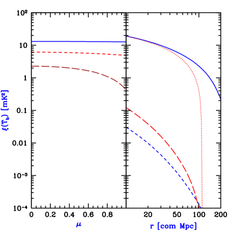
Figure 3: Correlation function of 21cm brightness temperature, same as Figure 2, except near the end of reionization ($\bar{x}_{n}=0.05$) by Pop II stars

Figure 4 summarizes the evolution of the 21cm correlation function during the latter half of the reionization epoch. Early in reionization, ionization affects only the rare high-density regions, and the anticorrelation of $\bar{x}_{n}$ and $\bar{\delta}$ leads to a low $\xi$ even though the cosmic mean brightness temperature is relatively high. Later on, as reionization spreads to more typical regions, $\bar{\delta}$ fluctuations produce amplified $\bar{x}_{n}$ fluctuations and $\xi$ increases, only to decrease at the end of reionization when the cosmic mean $x_{n}$ approaches zero. The anisotropy is most easily observable during the late stages where the signal is above 1 mK and is highly anisotropic. Note that the anisotropy is stronger in the case of Pop III stars, since in that case reionization occurs at a higher redshift and is caused by rarer halos, whose number density changes more rapidly with redshift during reionization.

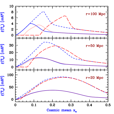
Figure 4: Correlation function of 21cm brightness temperature as a function of the cosmic mean neutral fraction $x_{n}$. Each panel corresponds to a comoving distance $r$ as indicated. We consider Pop II stars and an angle of $\mu=0$ (solid curves) or 1 (dotted curves), or Pop III stars and an angle of $\mu=0$ (short-dashed curves) or 1 (long-dashed curves).

4 Conclusions

At the later stages of reionization, ionization fluctuations dominate the 21cm power spectrum (Figures 2 and 3) and the light travel-time delay generates a strong anisotropy. The signal is around a few mK on scales and redshifts where the time-delay anisotropy is large (Figure 4), while noise and foreground-subtraction should still allow even first-generation 21-cm experiments to reach a sensitivity $\sim 1$ mK on large scales (Bowman et al., 2006; McQuinn et al., 2006).

The strong line-of-sight anisotropy in the ionization fluctuations arises in our model since the cosmic mean neutral fraction changes rapidly with redshift and its fluctuations are highly non-linear. The scale and angular dependence of the light-cone anisotropy must be modelled carefully in order to separate the inflationary initial conditions from astrophysical effects (Barkana & Loeb, 2005a). Large-scale numerical simulations of reionization (Iliev et al., 2006) could provide guidance for this difficult task, but fully self-consistent simulations with hydrodynamics and radiative transfer are required. Alternatively, the separation of the “physics” (i.e., the inflationary initial conditions) from the “astrophysics” may require observations at higher redshifts, when the neutral fraction is closer to unity and the 21cm power spectrum is dominated by density and peculiar velocity fluctuations.

References

- Barkana (2006) Barkana, R. 2006, MNRAS, submitted; astro-ph/0508341
- Barkana & Loeb (2001) Barkana, R., & Loeb, A. 2001, Phys. Rep., 349, 125
- Barkana & Loeb (2004) ——————————–. 2004, ApJ, 609, 474
- Barkana & Loeb (2005a) ——————————–. 2005a, ApJL, 624, L65
- Barkana & Loeb (2005b) ——————————–. 2005b, ApJ, 626, 1
- Barkana & Loeb (2005c) ——————————–. 2005c, MNRAS, 363, L36
- Bharadwaj & Ali (2004) Bharadwaj, S. & Ali, S. S. 2004, MNRAS, 352, 142
- Bond et al. (1991) Bond, J. R., Cole, S., Efstathiou, G., & Kaiser, N. 1991, ApJ, 379, 440
- Bowman et al. (2006) Bowman, J. D., Morales, M. F., & Hewitt, J. N. 2006, ApJ, 638, 20
- Bromm & Larson (2004) Bromm, V., & Larson, R. 2004, ARA& A, 42, 79
- Furlanetto, Zaldarriaga, & Hernquist (2004) Furlanetto, S. R., Zaldarriaga, M., & Hernquist, L. 2004, ApJ, 613, 1
- Iliev et al. (2006) Iliev, I. T., Mellema, G., Pen, U., Merz, H., Shapiro, P. R., & Alvarez, M. A. 2006, MNRAS, 369, 1625
- Jenkins et al. (2001) Jenkins, A., et al. 2001, MNRAS, 321, 372
- Loeb & Zaldarriaga (2004) Loeb, A., & Zaldarriaga, M. 2004, Physical Review Letters, 92, 211301
- Madau et al. (1997) Madau, P., Meiksin, A., & Rees, M. J. 1997, ApJ, 475, 429
- Madau et al. (2004) Madau, P., Rees, M. J., Volonteri, M., Haardt, F., & Oh, S. P. 2004, ApJ, 604, 484
- McQuinn et al. (2006) McQuinn, M., Zahn, O., Zaldarriaga, M., Hernquist, L., & Furlanetto, S. R. 2006, ApJ, submitted; astro-ph/0512263
- Nusser (2005) Nusser, A. 2005, MNRAS, 364, 743
- Scalo (1998) Scalo, J. 1998, in ASP conference series Vol 142, The Stellar Initial Mass Function, eds. G. Gilmore & D. Howell, p. 201 (San Francisco: ASP)
- Scott & Rees (1990) Scott, D. & Rees, M. J. 1990, MNRAS, 247, 510
- Sheth & Tormen (1999) Sheth, R. K., & Tormen, G. 1999, MNRAS, 308, 119
- Spergel et al. (2003) Spergel, D. N., et al. 2003, ApJ, 148, 175
- Wyithe & Loeb (2004) Wyithe, J. S. B., & Loeb, A. 2004, Nature, 432, 194
- Wyithe & Loeb (2005) Wyithe, J. S. B., & Loeb, A. 2005, ApJ, 625, 1
- Zaldarriaga, Furlanetto, & Hernquist (2004) Zaldarriaga, M., Furlanetto, S. R., & Hernquist, L. 2004, ApJ, 608, 622