INTEGRAL and RXTE Observations of Centaurus A

Abstract

INTEGRAL and RXTE performed three simultaneous observations of the nearby radio galaxy Centaurus A in 2003 March, 2004 January, and 2004 February with the goals of investigating the geometry and emission processes via the spectral/temporal variability of the X-ray/low energy gamma ray flux, and intercalibration of the INTEGRAL instruments with respect to those on RXTE. Cen A was detected by both sets of instruments from 3–240 keV. When combined with earlier archival RXTE results, we find the power law continuum flux and the line-of-sight column depth varied independently by 60% between 2000 January and 2003 March. Including the three archival RXTE observations, the iron line flux was essentially unchanging, and from this we conclude that the iron line emitting material is distant from the site of the continuum emission, and that the origin of the iron line flux is still an open question. Taking X-ray spectral measurements from satellite missions since 1970 into account, we discover a variability in the column depth between 1.0$\times 10^{23}\rm cm^{-2}$ and 1.5$\times 10^{23}\rm cm^{-2}$ separated by approximately 20 years, and suggest that variations in the edge of a warped accretion disk viewed nearly edge-on might be the cause. The INTEGRAL OSA 4.2 calibration of JEM-X, ISGRI, and SPI yields power law indices consistent with the RXTE PCA and HEXTE values, but the indices derived from ISGRI alone are about 0.2 greater. Significant systematics are the limiting factor for INTEGRAL spectral parameter determination.

1 Introduction

At a distance of $\sim$3.5 Mpc (Hui et al., 1993), the radio galaxy Centaurus A is one of the nearest and brightest active galactic nuclei (AGN). Since its discovery over three decades ago (Bowyer et al., 1970) (Note, however, Byrum, Chubb & Friedman 1970), many X-ray to gamma-ray instruments have shown it to have non-thermal, power law emission extending to the MeV range (Baity et al., 1981; Steinle et al., 1998). Hubble Space Telescope (HST) observations have revealed evidence for a small ($\sim$40 pc), inclined disk of ionized gas (Schreier et al. 1998) around a $\sim$$10^{9}$ M_⊙ black hole, and perhaps a region near the black hole evacuated by the jet (Marconi et al., 2000). Karovska et al. (2003) suggested that mid-IR observations resolved the nuclear region of size $\sim$3 pc, and together this might explain the lack of a hidden broad line region in Cen A (Alexander et al., 1999).

The power law index of Cen A below 100 keV has remained at $\sim 1.8$ for the last 40 years with the exception of 1972–1973 when OSO-7 found the index to be $\sim 1.2-1.4$ (Winkler & White, 1975; Mushotzky et al., 1976). The X-ray spectrum does not show any reflection component or a significant broad iron K$\alpha$-line (Woźniak et al., 1998; Rothschild et al., 1999; Benlloch et al., 2001), and yet it is rapidly variable (Morini, Anselmo & Molteni, 1989). This would imply, in contrast to radio-quiet Seyfert galaxies, that a cold accretion disk extending down close to the black hole may not be the source of the high energy radiation and the reprocessor is relatively far away. Furthermore, the hard X-ray spectra of individual Seyfert 1s show an underlying continuum which is a power law, with a nearly exponential rolloff with a folding energy of $\sim$100–300 keV (Johnson et al., 1997). Cen A, on the other hand, does show $\sim$MeV range emission, thereby indicating it is quite different from the radio-quiet Seyferts.

Current observations of Cen A are presented in § 2, and the methods of analyzing both the INTEGRAL and RXTE data will be found in § 3. In § 4 we present the results from fitting the combined instrument data from each mission from the 3 simultaneous observations and from reanalyzing the 3 previous RXTE observations with HEASOFT release (5.3.1). In § 5 we use these results to discuss the emission processes in the nuclear region of Cen A, and present our conclusions in § 6. We present an extensive analysis of each instrument’s response to Cen A as well as an inter-calibration of the 2 missions in the Appendix. Included in the Appendix is also a study of the stability of the PCU2 calibration over the RXTE mission as determined from observations of Cas A.

2 Simultaneous INTEGRAL/RXTE Observations

INTEGRAL and RXTE observed Cen A three times as part of the INTEGRAL AO-1 and RXTE AO-7 proposal cycles in March 2003 and early 2004. The INTEGRAL observations utilized the Joint European X-ray Monitor (JEM-X; Lund et al., 2003), the Integral Soft Gamma-Ray Imager (ISGRI; Ubertini et al., 2003) portion of the Imager onBoard the INTEGRAL Satellite (IBIS), and the SPectrometer on board INTEGRAL (SPI; Vedrenne et al., 2003). The RXTE observations used the Proportional Counter Array (PCA; Jahoda et al., 1996) and the High Energy X-ray Timing Experiment (HEXTE; Rothschild et al., 1998). Table 1 gives the details of these three observations plus the previous three RXTE observations (Benlloch et al., 2001). The INTEGRAL observations are essentially continuous due to the $\sim$72 hr elliptical orbit, while the RXTE observations are broken-up due to South Atlantic Anomaly passages, Earth-occults, and unavoidable slews to other targets for short periods of time. Consequently, livetimes for INTEGRAL instruments are greater than those for RXTE. The single RXTE proportional counter PCU2 has 14 times the background-subtracted counting rate of the JEMX-2 detector, and HEXTE has 95% of the ISGRI background-subtracted counting rate. As seen below, the small PCU2 and HEXTE fields of view ($\sim 1^{\circ}$ FWHM) and low backgrounds result in RXTE-derived spectral parameters with significantly smaller uncertainties than those derived from INTEGRAL spectral data.

3 Data Analysis Methods

The analysis of the data from the INTEGRAL instruments used the Off-line Scientific Analysis (OSA) 4.2, and followed the OSA 4.2 procedures outlined in the various instrument analysis user manuals. Specifically, coded mask deconvolution, as opposed to the open/closed pixel method, was used. The RXTE instruments analysis was based upon the Warwick/Tübingen/UCSD scripts that make use of the HEASARC-provided RXTE FTOOLS of HEASOFT release 5.3.1.

Due to the variable number of PCUs on at any one time, data for all observations were available only for PCUs 0 and 2. We chose to limit the detector selection further to just PCU2, since PCU0 had lost its propane veto layer in the Spring of 2000 (Jahoda et al., 2004), and calibration/background estimates for PCU0 were not as mature as those for PCU2.

An absorbed power law plus narrow iron line spectral model (phabs*(power + gauss)) has been used to represent the flux from Cen A for all observations. Since JEM-X did not detect the iron line seen by the PCA, and since large JEM-X residuals prevented meaningful estimation of upper limits to the line flux, the line was not included in the INTEGRAL fitting. The following energy ranges were used in the fitting process: PCU2 (2.5–60 keV), HEXTE (17–240 keV), JEM-X (3–30 keV), ISGRI (22.5–100 keV), and SPI (20–250 keV). No systematic errors have been added to the SPI or HEXTE data. We have added 0.3% systematic errors to the PCU2 data in order to obtain $\chi^{2}_{\nu}$ values near 1, since the statistical errors are very much smaller than the systematic ones. This is consistent with suggested systematic errors from fitting the Crab (Jahoda et al., 2004). (See Appendix B for a discussion of additional specific PCU2 systematic effects that were modeled as part of the fitting procedure.) On the other hand, we have had to add systematic errors to the ISGRI and JEM-X data due to incomplete modeling of the instrument/background response (see § 4.1.1 & 4.1.2). The observation-dependent systematic errors added to JEM-X and ISGRI data are given in Table 2. All errors quoted in this paper represent 90% confidence intervals, with the exception of 1$\sigma$ errors for counting rates that were generated by the SHOW RATE command in XSPEC. Errors on fluxes and equivalent widths for individual instrument fits were determined using the FLUX and EQW commands within XSPEC with the ERR option invoked using 500 trials. They rely on the assumption that the parameter value distribution is multivariate Gaussian centered on the best-fit parameters, and are only an approximation in the case that the fit statistic space is not quadratic. The PCU2 was taken to be the reference instrument when PCA/HEXTE spectra were fitted, and when only INTEGRAL data were analyzed, JEM-X spectra provided the reference flux.

The INTEGRAL data are comprised of a series of $\sim$2000 s Science Windows (ScWs) containing the science data. We investigated the significance of the 20–40 keV flux in the images from each ScW included in our observation with respect to Cen A. In Obs. 4, Revolution 48, ScWs 92–95 had questionable non-detections, assumed to be due to nearing passage through the radiation belts. These ScWs were not included in the analysis, while all others were. We also identified the ScWs that contained Cen A in the JEM-X field of view. A separate list of ScWs than for that of ISGRI and SPI was used for the JEM-X analysis, due to the smaller JEM-X field of view, and the fact that the dithering would move Cen A from the JEM-X field of view. Data were only accumulated from the inner $4^{\circ}$ radius region in JEM-X in order to avoid inclusion of spurious events from the edge of the detector system. Consequently, the amount of JEM-X data was less than that of ISGRI or SPI. No attempt was made to extract PICsIT spectra, since OSA 4.2 does not provide software for spectral extraction of PICsIT data. Counting rates and exposure times are given in Table 1.

The INTEGRAL observations were made using the dithering mode of INTEGRAL in which the field of view is stepped around a selected hexagonal pattern in 2^∘ steps. This is to help suppress systematic effects associated with background variations in SPI. The last third of Obs. 4 was taken in the staring mode where the satellite remained pointed directly at Cen A.

The RXTE data accumulations were restricted to times when Cen A was more than $10^{\circ}$ above the Earth’s limb from RXTE’s point of view, when RXTE was more than 30 minutes past the beginning of a South Atlantic Anomaly passage, when the pointing direction was within $0\fdg 01$ of the Cen A position, and when the PCU2 and HEXTE high voltages were at their nominal values.

3.1 INTEGRAL Imaging and Spectral Accumulations

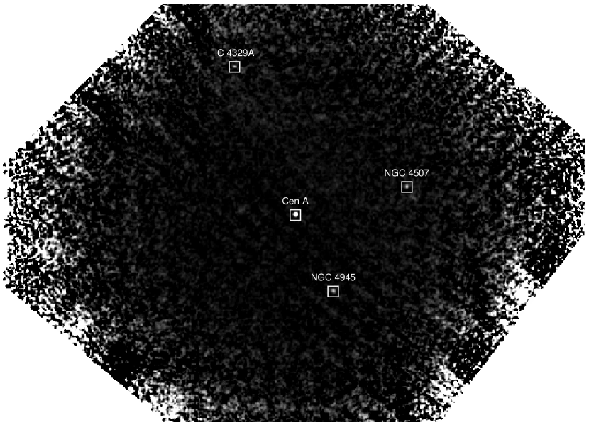
Figure 1: The 20–40 keV ISGRI image from Obs. 4, which shows Cen A, NGC 4945, and NGC 4509 as the three sources detected.

Since the ISGRI instrument presented the best view of the multi-source sky at 20 keV, it was used initially to form images of the field of view of each observation. Cen A, IC4329A, NGC 4945, and NGC 4509 were the only sources detected during the Cen A observations (Fig. 1). The catalog of sources used in subsequent analyses included only these 3 sources. In addition, FLAG and SEL_FLAG parameters in the catalog were set to 1 to force inclusion of data from portions of the telemetry where the source was in the field of view but might not meet the detection level criterion. In this manner, spectral data were accumulated from all available telemetry. This approach is essential to the proper measurement of the flux; using only the detections above a given threshold will bias the result to higher fluxes.

The JEM-X spectral histograms were rebinned from the original 256 channels covering 0-82 keV to 34 energy bins with $\sim 0.5$ keV/channel from 3–8 keV, and $\sim 1$ keV/channel from 8–30 keV. The ISGRI data were grouped into 30 energy bins that were initially 2 keV/channel at 22.5 keV and increased to 100 keV/channel for 200 keV and beyond. The present ISGRI analysis was limited, however, to 22.5–100 keV due to recommendations from the ISGRI team (P. Ubertini, private communication) and large residuals above 100 keV (see Appendix 4.1.2). The SPI data were logarithmically binned into 20 channels from 20–250 keV for the individual observations and no SPI channels were ignored in the analysis. The PCU2 spectral data were not rebinned. The HEXTE data remained at 1 keV/channel up to $\sim$50 keV, were then grouped at 5 keV/channel until $\sim$160 keV above which the binning was 10 keV/channel.

Cen A was also in the field of view during observations of NGC 4945 taken just after Obs. 5. We have extracted ISGRI and SPI spectra for this observation also (Cen A was always outside the JEM-X field of view) to determine if they could add to the present results. The lower statistical quality of these spectra due to the reduced off-target response did not justify their inclusion, but they did provide insight into results for sources NGC 4945 and NGC 4509 offset from the target direction during the present observations (see Appendix E).

3.2 RXTE Spectral Accumulations

The six spectral accumulations for both PCA and HEXTE were made using the Standard Data formats present in all RXTE observations, independent of the specific modes chosen by the observers. The PCA SkyVLE background model was used for PCA background subtraction, while the HEXTE realtime off-source observations provided the data for HEXTE background subtraction. The HEXTE instrument design includes continuous, automatic gain control which allows for the use of a single instrument response throughout the mission. The accumulation of background observations of four overlapping regions of the sky just beyond the source position minimizes any systematic effects due to temporal and spatial variations in the HEXTE background measurement within statistical uncertainties. Consequently, systematic uncertainties in HEXTE source spectra arise only from those in the instrument response to X-rays and the HEXTE deadtime calculation. The effect of the latter can be estimated by the size of the adjustment of the amount of measured background required in an iterative fitting process, as described for the PCU2 (Appendix B). For HEXTE, this yielded about (0.1$\pm$0.1)% at the 1$\sigma$ uncertainty level. The HEXTE data were collected in each cluster separately, and the two off-source positions for each cluster were checked for confusing source(s) by comparing rates. Upon finding no evidence for such sources, the two off-source regions of each cluster were added to form each cluster’s background spectrum. Then both the source and background spectral data from the two clusters were combined to form a single set of HEXTE source and background files for analysis.

4 Spectral Analysis of INTEGRAL and RXTE Data

4.1 INTEGRAL Results

4.1.1 Fitting JEM-X

The best-fit parameters without additional systematic errors for an absorbed power law model for the JEM-X observations of Cen A are given in Table 2 and the resulting spectra are shown on the left hand side of Fig. 2. Comparing the residuals to the fits in the three spectra reveals a broad feature centered at $\sim$7 keV, which may be the combination of two narrow lines, in the latter two observations. A third line-like feature is also seen in the Obs. 6 residuals near 20 keV. Two approaches were tried to address the systematics in the spectral analysis: 1) the addition of Gaussian components in the spectral model, and 2) the addition of systematic error to the spectral data (see Appendix D). Since the first observation has no strong evidence of these two lines, we speculate that they are associated with a gain variation with time that is not included in the JEM-X instrument response calculation. As discussed in Appendix D, the latter prescription of adding systematic errors to the data to achieve $\chi^{2}_{\nu}\approx 1$ was found to be preferable. The results of fitting with systematic errors added are given in Table 2 and shown on the right hand side of Fig. 2. The mean column density $\langle N_{\rm H}\rangle$=13.8${}^{+5.5}_{-4.6}\times 10^{22}$ cm^-2 and the mean power law index $\langle\Gamma\rangle$=1.80${}^{+0.17}_{-0.17}$ for the 3 JEM-X observations. The 3 individual values of $N_{\rm H}$ and of $\Gamma$ are consistent with the respective mean values at the 90% confidence level. Thus, only variations in the overall flux were detected by JEM-X.

4.1.2 Fitting ISGRI

The ISGRI spectra were initially fit to the full 13-400 keV energy range to determine the extent of significant detections of Cen A. As seen in Fig. 3 (Left), very significant residuals to the fit are present below $\sim 30$ keV, near 60 keV, and between 100 and 150 keV. These residuals are present in all 3 observations to some extent. The analysis energy range was then reduced to 22.5–100 keV to concentrate on the high statistical significance portion of the data, and the fitting was redone. Since the energy range of ISGRI precluded determination of the line of sight column depth, the JEM-X value for each observation was used. Table 2 gives the best-fit spectral parameters for the case of no systematic errors added to the data, and for the case when they were added to achieve $\chi^{2}_{\nu}\approx 1$. The trend, however, was to require more systematic errors for the later observations (3.5% for Obs. 4, 7.5% for Obs. 5, and 9.5% for Obs.6). This may indicate a time-dependent calibration is required for ISGRI analysis. Fig. 3 (Right) shows the 22.5–100 keV ISGRI spectra with systematics for the 3 observations. The mean value of the power law index $\langle\Gamma\rangle$=2.01${}^{+0.09}_{-0.09}$, and the 3 individual values of $\Gamma$ are consistent with this mean value. The observation-to-observation flux variation seen by JEM-X is also present in the ISGRI results.

4.1.3 Fitting SPI

The SPI data were initially accumulated over the 20–600 keV range, again, to understand the range of detection of Cen A. This resulted in our choice to analyze the SPI data from 20–250 keV in 20 logarithmically spaced bins. As was true for ISGRI, the JEM-X value for the line of sight absorption was used in fitting each SPI histogram. The 3 SPI spectra are shown in Fig. 4 and the best-fit parameters are given in Table 2. The range of reduced $\chi^{2}$ was 0.45$<\chi^{2}_{\nu}<$1.10 and thus there was no need for any additional systematic uncertainties to be added. The mean power law index $\langle\Gamma\rangle$=1.78${}^{+0.17}_{-0.17}$, and the 3 individual values are consistent with this value. SPI fluxes reflected those seen by JEM-X.

4.2 RXTE Results

4.2.1 Fitting PCU2

The residuals to initial fits to PCU2 data and the procedures to address the systematic effects causing them are discussed in Appendix B. By applying these procedures, the entire 2.8–60 keV energy band of the PCU2 becomes available for analysis, and at the same time, this expands the overlapping coverage of PCU2 and HEXTE to 17-60 keV. Table 3 gives the resulting best-fit spectral parameters for the PCU2 observations of Cen A, along with the percent corrections made to the background to enable a best-fit. Corrections to the PCU2 background estimate are at the few percent level with 1$\sigma$ uncertainties of a few tenths of a percent. This allows for measurement of continuum parameters and iron line centroids to $\sim$1%, and iron line fluxes to $\sim$5%. The resulting best-fit spectra are shown in Figs. 5 & 6. In the first 3 observations, the mean column density and power law index are $\langle N_{\rm H}\rangle$=9.97${}^{+0.27}_{-0.26}\times 10^{22}$ cm^-2 and $\langle\Gamma\rangle$=1.834${}^{+0.009}_{-0.032}$, and the three individual measurements of $N_{\rm H}$ and $\Gamma$ are consistent with the respective mean values. In the simultaneous INTEGRAL/RXTE observations, $\langle N_{\rm H}\rangle$=15.86${}^{+0.22}_{-0.21}\times 10^{22}$ cm^-2 and $\langle\Gamma\rangle$=1.829${}^{+0.011}_{-0.008}$, and again no variation in $N_{\rm H}$ or $\Gamma$ is detected for the last 3 observations. When comparing Obs. 1–3 and 4–6 , we find that the power law indices are consistent with no change, but the column densities show a 60% increase. No correlation is seen between the 2–10 keV flux and the column density.

4.2.2 Fitting HEXTE

Table 3 gives the best fit parameters for the six HEXTE spectra along with the percentage background adjustments. We find an average of 0.15%$\pm$0.12% adjustment to background, and are able to achieve 1.01$<\chi^{2}_{\nu}<$1.25 when fitting the Cen A observational data without application of any additional systematic errors. The resulting best-fit spectra are shown in Figs. 5 & 6. The mean power law from the first 3 observations $\langle\Gamma\rangle$=1.83${}^{+0.07}_{-0.07}$ and in the simultaneous INTEGRAL/RXTE observations $\langle\Gamma\rangle$=1.79${}^{+0.02}_{-0.02}$. These values are consistent with their counterparts from the PCU2 data.

4.3 Analysis of INTEGRAL/RXTE Results

Comparing the best-fit values from the RXTE observations allows for long term variability to be assessed, and comparing INTEGRAL and RXTE results on the last 3 observations is the basis for evaluating the INTEGRAL/RXTE instrument cross calibration.

4.3.1 Instrument Cross-Calibration

The effective areas of the PCA and HEXTE on RXTE have been extensively calibrated in the laboratory and in orbit with present day residuals to spectral fitting at the percent level or less. Similarly, the INTEGRAL instruments have had extensive ground calibrations; however, the absolute effective area of each instrument, the in-orbit instrument response, and the instrumental background subtraction technique are still being addressed through regular OSA releases.

For intercomparison of individual instruments, the RXTE/PCU2 is assumed to provide the “true” values of column density and power law index. The mean PCU2 column density for Obs. 4-6 is 15.86${}^{+0.26}_{-0.22}\times 10^{22}$ cm^-2 and the mean best-fit JEM-X value is 13.8${}^{+5.5}_{-4.6}\times 10^{22}$ cm^-2. From this we see that the JEM-X value is consistent with the PCU2 value at the 90% confidence level, and the PCU2 is 20 times more sensitive to column density in this instance. Comparison of the mean power law indices reveals that JEM-X and SPI agree easily with PCU2 due to their relatively large uncertainities of 0.17 for indices of 1.80 and 1.78, respectively, but that the mean ISGRI best fit index is 0.18$\pm$0.09 larger. Averaged over the first 3 observations, HEXTE and PCU2 power law indices are nearly identical (1.830${}^{+0.071}_{-0.075}$ vs. 1.834${}^{+0.009}_{-0.032}$), and are a bit farther apart in the second set of three observations (1.794${}^{+0.018}_{-0.018}$ vs. 1.825${}^{+0.012}_{-0.010}$). Overall, PCU2 is nearly an order of magnitude more sensitive to the power law index than the INTEGRAL instruments.

Simultaneous fitting of PCU2 and HEXTE provides for the RXTE best-fit spectral results over the full 2.8–240 keV range and also yields the HEXTE-to-PCU2 normalization. Simultaneous fitting of JEM-X, ISGRI, and SPI spectra provides the 3–250 keV INTEGRAL result and normalizations. Table 4 gives the best-fit Cen A spectral parameters for INTEGRAL and RXTE. These results may differ from those from individual instrument fits, since they force a single power law to be used, and since column density and power law index are correlated.

The three INTEGRAL instrument effective areas were compared to RXTE by fitting the INTEGRAL data with “frozen” RXTE best-fit spectral parameters, including normalization of the power law. A variable constant for each INTEGRAL instrument’s flux was used to compute their relative normalizations to RXTE. In this manner, one finds the relative normalization of each instrument with respect to RXTE. JEM-X relative to RXTE averages about 90%, ISGRI about 84% and SPI about 109%. HEXTE averaged 92% of PCU2 over the 6 observations.

5 Results on Cen A

5.1 Previous Observations

In the years preceeding the present observations, the instruments on BeppoSAX and RXTE viewed Cen A five times (Grandi et al., 2003) and three times (Benlloch et al., 2001), respectively. In the energy range above 3 keV, they found the spectrum to be characterized by an absorbed (N${}_{H}\sim$10²³ cm^-2) power law ($\Gamma$=1.80). Simultaneous BeppoSAX/CGRO observations, revealed the spectrum to steepen exponentially (e-folding energy $\sim$600 keV). The 1991 flight of the Welcome-1 balloon found evidence for a break, or roll over in the spectrum at 150–200 keV (Miyazaki et al., 1996), whereas the LEGS balloon (70–500 keV) and reanalysis of HEAO-1 measurements (2 keV to 2 MeV) of Cen A did not require a low energy break (Baity et al., 1981; Gehrels et al., 1984).

Ginga/OSSE, and RXTE found no evidence for a Compton reflection component implying little cold, Thomson-thick material in the close vicinity of the AGN or radiation beamed away from the accretion disk (Woźniak et al., 1998; Rothschild et al., 1999; Benlloch et al., 2001). The strongest upper limits to date on the solid angle contributing to the reflection are $\Omega/2\pi<0.05$ from the combined RXTE observations (Benlloch et al., 2001).

Recently Chandra and XMM-Newton observations have allowed the separation of the nuclear component from that of the jet and galactic flux (Evans et al., 2004). These observations resolve the Fe line and find fluorescent K_α emission from cold neutral or near-neutral iron with a line width of $\sim$20 eV. This is consistent with emission from material at a large distance from the site of the hard X-ray emission. The lack of change in the flux of the Cen A iron line over 20 years despite significant changes in the strength of the observed hard X-ray continuum (Rothschild et al., 1999), supports this suggestion that the absorbing/fluorescing material is at least several parsecs from the central engine or insensitive to contunuum variations (e.g. Miniutti et al., 2003).

5.2 Cen A Spectral Results

With respect to variations in Cen A, the power law index, the iron line centroid, and the iron line flux showed no indication of significant variability over the 6 RXTE observations (Table 4). The column density, however, was constant in the pre-2000 observations and again constant in the post-2000 observations, with a significant 60% increase between January 2000 and March 2003 — (10.0$\pm$0.2)$\times 10^{22}$ cm^-2 to (15.9$\pm$0.2)$\times 10^{22}$ cm^-2. In conjunction with this variation in column density, no similar change in iron line flux was detected. A maximum change of 39% (4.0$\times 10^{-4}$ cm^-2 s^-1 to 5.7$\times 10^{-4}$ cm^-2 s^-1) in the line flux is the largest allowed within 90% confidence. The present finding of constant column density in the 3 earlier RXTE observations compared to the claim of variation by Benlloch et al. (2001) can be attributed to the new calibration (HEASOFT 5.3.1) and to the ability to analyze PCU2 data to 60 keV.

The PCU2 measured iron line centroid had a mean of 6.42${}^{+0.08}_{-0.04}$ keV over the first 3 observations and 6.33${}^{+0.07}_{-0.02}$ keV over the second 3. These two values are consistent with 90% confidence, and the mean over all 6 observations is 6.38 keV with a standard deviation of 0.07 keV. The standard deviation value represents a 1% measurement that is consistent with calibration uncertainties and other systematic effects in PCU2 analysis (see Appendix C). The Fe K$\alpha$ line is therefore consistent with emission from a neutral medium.

The flux of the iron line had a mean value of 4.43${}^{+0.53}_{-0.50}\times 10^{-4}$ cm^-2 s^-1 for the first 3 observations and 5.13${}^{+0.55}_{-0.52}\times 10^{-4}$ cm^-2 s^-1 in the second three. Thus, no significant flux variability is detected, as the two values are consistent at the 90% confidence level. The mean of all 6 observations is 4.77$\times 10^{-4}$ cm^-2 s^-1 with a standard deviation of 0.70$\times 10^{-4}$ cm^-2 s^-1. While the standard deviation is about 40% larger than the 90% statistical uncertainties, it only represents about 15% of the flux.

The 2–10 keV flux had a factor of 2 range of (1.69–3.22)$\rm\times 10^{-10}ergs\;cm^{-2}s^{-1}$, and no correlation is seen between flux and power law index, iron line energy, or iron line flux.

5.3 Cen A Lightcurves

Background subtracted light curves were generated for the full PCU2 energy range with 1024 s time resolution to study temporal variability over each observation. These light curves are shown in Fig. 7. Quarter hour and day-to-day variability of $\sim$20% is clearly seen. Fig. 8 Top shows the relation between the On-source, background, and net Cen A counting rates for Obs. 5. The ratio of Cen A to background in PCU2 was $\sim 1$. Fig. 8 Bottom gives the light curve of Obs. 2 in more detail by splitting the observation into first and second halves, since a large gap in time was inserted into the observation to accomodate observing another source.

We used the 2.5–60 keV PCA light curves to produce a power density spectrum (PDS) for the full data set. We divided the 16 s time resolution light curves into 1008 s segments and calculated power spectra for each of the 245 segments. The 0.001-0.031 Hz PDS includes a total of 246,960 seconds of exposure time. First, we produced a Leahy-normalized PDS (Leahy et al., 1983), and then we subtracted-off the Poisson level and re-normalized to obtain the rms-normalized PDS (Miyamoto et al., 1991) shown in Fig. 9. The PDS is relatively well-described ($\chi^{2}_{\nu}$ = 27/20) by a power-law function with a slope of $\alpha=2.36\pm 0.15$, and the 0.001-0.03 Hz fractional rms is 1.59%$\pm$0.06%. There is some evidence for excess power around 0.018 Hz, but the quality of the power spectrum is poor above $\sim$0.008 Hz.

5.4 Search for Spectral Breaks in Cen A

In order to test for breaks or curvature in the Cen A continuum, we fit the three observations with the largest livetime $\times$ PCU2 count rate product to give the best statistical result (Obs. 4, 5, & 2). In addition to the standard single power law, we tested a broken power law and a cut-off power law. For Obs. 2 testing of a broken power law, the fits were insensitive to the break energy and it was fixed at 100 keV. In each case the iron line and systematics parameters were essentially unchanged from the single power law case, and no significant improvement over the single power law was found. Table 5 shows the results of this testing. CGRO found a 1.74${}^{+0.05}_{-0.06}$ power law index from 50 to 150 keV, which then steepened to an index of 2.3${}^{+0.1}_{-0.1}$ (Kinzer et al., 1995) when the source flux was comparable to the present Obs. 4. CGRO found a lesser steepening ($\Delta\Gamma$=0.24$\pm$0.10) when the flux was lower by a factor of 0.6, and comparable to Obs. 2. While RXTE yields results consistent with those of CGRO, the RXTE spectra do not require the presence of a break.

All 6 HEXTE data sets were summed together to give the highest statistical sensitivity at high energies, and tested again for a break. Nothing significant was found. The summed HEXTE spectrum is shown in Fig. 10. No deviation from a single power law to 200 keV was detected.

5.5 Spectra of Three AGN in the Field

IC4329a, NGC 4945 and NGC 4507 were in the field of view of ISGRI and SPI during the Cen A observations, and as a result, data are available for them. Their 30–70 keV count rates ranged from 0.6–2 c/s, and detailed spectral analysis was not practical. We fit the Obs. 4 spectra with a power law and used the resulting best-fit indices to calculate the 20-100 keV flux for each object. Table 6 gives the rates and fluxes for both objects for the 3 INTEGRAL observations. The errors given are 1$\sigma$. From this we can conclude that NGC 4945 varied up and down by $\pm$25%, NGC 4507 declined over the 3 observations by 50%, and IC4329a essentially was constant. As presented in Appendix E, no additional systematic effects — just lower statistical significance due to lower counting rates — affected these measurements. The fluxes and power law indices are good indications (within statistical uncertainties) of the emission from NGC 4945, NGC 4507, and IC4329a at the time of the Cen A observations.

6 Discussion

Over the last 3 decades, Cen A has been observed from space by nearly all X-ray and gamma ray missions. Fig. 11 shows the measured values of the inferred column density, $N_{\rm H}$, since 1975 (see also Risaliti, Elvis, & Nicastro, 2002). The lower value of $\sim$10$\times 10^{22}$ cm^-2 is seen to occur twice in this time period, with the higher value of $\sim$15$\times 10^{22}$ cm^-2 seen the rest of the time. The first occurrence of the lower value was detected by only HEAO-1 in 1978, while the second was seen by RXTE, Chandra, and BeppoSAX. One can estimate the duration of the second occurrence of low column depth to be about 3000 days or 8 years. The duration of the first occurrence could also have lasted this long, but no observations were made in the early ’80s. The transition from low to high absorption, which may have been resolved in 2002-2004, took about 2 years. The range of high values of $N_{\rm H}$ seen from $\sim$(13.5 to 17)$\times 10^{22}$ cm^-2 is broader than the range of lower values, (9.5 to 10.2)$\times 10^{22}$ cm^-2, and this might indicate that the lower values represent the baseline for judging variations in column depth. The times of increased absorption could represent dense ($\sim 10^{22}$ cm^-2) clouds transiting the line of sight, or variable structure in the outer edges of the obscuring accretion disk or molecular torus. If the $\sim$9 year duration of the higher level of absorption seen in the center of Fig. 11 represents a cloud, and if, as discussed by Wang et al. (1986), it resides in the broad line region at 10¹⁷ cm from the central object and has velocity of 500–1000 km/s, its diameter would be $\sim$10¹⁷ cm — the size of the entire broad line region. If we assume a more reasonable cloud of diameter of 10¹³ cm and $N_{\rm H}=5\times 10^{22}$ cm^-2, then its velocity would be a meager 0.3 km/s and would place the cloud far beyond the core region. A cloud-based explanation appears to be untenable.

The second possibility is variable structure in the outer edge of the disk. This could be characterized as a non-uniform edge structure that rotated through the line of sight as the outer disk rotated or just stochastic variations in disk structure. Assuming a 2$\rm\times 10^{8}M_{\odot}$ black hole (Silge et al., 2005), 20 pc radius accretion disk (Schreier et al., 1998), and Kelperian motion, the velocity of the outer edge of the disk is $\sim 7\times 10^{6}$ cm s^-1 and the circumference is $\sim 4\times 10^{21}$ cm. A point on the edge will travel 2$\times 10^{15}$ cm in 8 years, or less than a millionth of the circumference. Thus, the required structure is quite small with respect to the disk, and is not out of the question. Another possible explanation is precession of the warped accretion disk (Schreier et al., 1998) creating a variable absorption. The lower column depth would represent the time when the edge of the disk raised or lowered to allow a more direct view of the emission region, and the higher values could be associated with the edge of the disk returning to attenuate the X-ray emission.

While the changes in the column depth are clear and dramatic over the past 30 years, the behavior of the inferred power law index is less so. Fig. 12 displays the power law indices versus time for the same missions as Fig. 11. While the index was less than 1.7 during the OSO-8/HEAO-1 era, the index is seen to be consistent with 1.8 since 1989 (Ginga). The column depth is not correlated with the power law index, since the $N_{\rm H}=10\times 10^{22}$ cm^-2 and $\Gamma<$1.7 condition was not repeated in the RXTE/BeppoSAX era when the 50% increase in $N_{\rm H}$ occurred. The power law index at that time did not change from 1.83. This fact is further strengthened by the fact that the two values of $N_{\rm H}$ and the single value of $\Gamma$ were measured by the same instrument set on RXTE, and henceforth possible systematic effects relating to differing calibrations on different spacecraft are not a factor. From this we conclude that the primary emission region producing the power law component is independent of the absorbing region.

We also note that the X-ray telescopes ASCA, Chandra and XMM-Newton have larger uncertainties in their determination of the continuum than the non-imaging missions with energy ranges extending to higher values. This highlights the importance of simultaneous broadband X-ray coverage of XMM-Newton and Chandra observations of bright sources, such as black hole transients and accreting X-ray pulsars where detailed knowledge of the continuum is essential.

No correlation is seen between flux and power law index, and no large variation in iron line flux is seen since 1984, while the inferred absorbing column varied by 60%. The flux of the power law continuum varied a factor of two or more during this time with no accompanying variation in the line flux (Fig. 13). Two possible sources of the iron line flux are a reflection component (e.g., George & Fabian, 1991) or transmission through the obscuring matter (e.g., Miyazaki et al., 1996). Both scenarios, however, are not consistent with the observations. The reflection component is attractive, since calculations by Miniutti et al. (2003) show that the power law component can exhibit large variations due to the position of the primary emission above the accretion disk while the iron line flux variations would be an order of magnitude less. A reflection component is not required from the spectral analysis (Benlloch et al., 2001), however, and thus the contribution to the observed iron line flux would be minimal. On the other hand, transmission through a line-of-sight absorbing medium (outer edge of an accretion disk or an obscuring torus) would predict that the equivalent width would vary with column depth with an equivalent width of $\sim$100 eV for $N_{\rm H}\approx 1\times 10^{23}$ cm^-2 (Miyazaki et al., 1996). Obs. 1–3 as well as Obs. 4–6 find a factor of 2 variation in the equivalent width for constant values of the column depth of 1 and 1.5 $\times 10^{23}$ cm^-2, respectively.

If a distant iron emitting region were illuminated by beamed emission and the continuum was produced relatively near the black hole, the sparse sampling of Cen A would not have been expected to reveal correlated behavior. This physical separation would easily support the observation of reduced equivalent widths with increased continuum flux, as seen in each set of 3 observations by RXTE that are characterized by a single value of the column depth. If the iron line flux represents a measure of the beamed flux, estimates of the line flux indicate that the jet luminosity is on the order of the X-ray continuum luminosity from the Cen A core. If this hypothesis is correct, we can infer that the beamed flux variability, on the average, is less variable than that of the X-ray flux on the timescale of the 6 RXTE observations.

7 Conclusions

The six RXTE observations over the last nine years have shown that the 3–240 keV Cen A spectrum can be described by a single absorbed power law plus an iron emission line. We have measured the column density to Cen A to about 1%, the power law index and iron line centroid energy to better than 1%, and the iron line flux to approximately 10%. While still systematics dominated, INTEGRAL determines the power law index to a few percent and the column depth to 10–20% from simultaneous observations with the last three RXTE observations in 2003 and 2004. We have provided an in depth comparison of RXTE and INTEGRAL instruments using the latest knowledge of the instrument responses and techniques for addressing systematic errors. Appendix F gives the improved INTEGRAL spectral results using OSA 5.0 analyzed after submission of this paper.

The mean values of $N_{\rm H}$ and $\Gamma$ resulting from the spectral analyses of individual instruments on INTEGRAL and RXTE and of simultaneous fitting of all insturments on a given satellite are given in Table 7. All five instruments’ spectral parameters are in agreement at the 90% confidence level, except for the ISGRI determination of the power law index. The ISGRI value of $\Gamma$ is significantly larger ($\Delta\Gamma\sim$ 0.2$\pm$0.1). This discrepancy is $\sim 0.1$ using OSA 5.0.

From the RXTE observations, we have detected a 60% increase in the mean column depth to Cen A between 2000 and 2003, and this increase was not correlated to either the spectral index or the 2–10 keV flux. The increase in column depth was accompanied with a small drop in iron line flux that is not significant at the 99% confidence level. By considering past satellite measurements of the absorbing column, we note two episodes of $N_{\rm H}=1.0\times 10^{23}\rm cm^{-2}$ separated by $\sim$20 years, and speculate that variability in the structure of the outer edge of the warped accretion disk could explain the observed variability. Since the continuum shape and iron line flux did not vary significantly, we suggest that they are separate from each other and the intervening material.

Where, then, does the Fe K$\alpha$ line originate? Since the line strength does not correlate with $N_{\rm H}$, we do consider it unlikely that the Fe line is produced in the absorbing material. The similarity of the Cen A line parameters with those now seen with Chandra or XMM-Newton in many AGN, low-luminosity Seyferts, and high-luminosity QSOs, which all have narrow lines (to the resolution of the observation) at an energy consistent with emission by neutral Fe and equivalent widths of less than about 150 eV (see, e.g., Pounds & Reeves, 2002; Yaqoob & Padmanabhan, 2004; Reynolds et al., 2004; Jiménez-Bailón et al., 2005) points at a similar origin for these features. The line parameters are characteristic for a line origin as a fluorescence line in material that is irradiated by X-rays. The possible location of the line emitting region is either the outer regions of the accretion disk or a medium separate from the disk, such as the torus posited in unifying models for AGN. As shown by Ghisellini, Haardt & Matt (1994) and Leahy & Creighton (1993), for parameters typically assumed for the torus and the central source, equivalent widths of 100 eV are expected. Alternatively, as discussed by Yaqoob et al. (2001) and Jiménez-Bailón et al. (2005), such lines could also originate in the broad line region, with the size of the region again being sufficiently large that one would not expect a correlation between the flux from the central source and the line strength.

We note, however, that the presence of a jet is one crucial difference between radio quiet Seyfert galaxies and objects such as Cen A or radio-loud QSOs. As has been recently shown for both Galactic black hole candidates and for low luminosity AGN, a significant fraction of the X-ray emission from these systems could also be explained by synchrotron-self Comptonization radiation from the base of the radio jet and thus not be due to thermal Comptonization (Markoff, Nowak & Wilms, 2005; Falcke, Körding & Markoff, 2004, and therein). The lack of a roll-over and reflection component in Cen A, as opposed to Seyfert galaxies, could therefore also be due to jet emission, with beaming or the small footprint of the jet reducing the amount of reflection expected. In these models, the advected flow at the base of the jet produces the hot electrons and SSC radiation could extend to high energies. In Seyfert galaxies, the jet could be less beamed/thermal, or thermal Comptonization could be more dominant, resulting in the observed roll-over. If this is the case, then the observed line emission could also originate from a region that, due to beaming, is significantly more illuminated by the jet than the disk. As we would not see the illuminating radiation but only the Fe K$\alpha$ emission, which is emitted isotropically, no correlation between the continuum and the Fe line flux would be expected. In addition, such a model could also explain the absence of hidden broad lines from radio galaxies like Cen A, as the jet may sweep out the material that otherwise would form the broad line region. It is beyond the scope of this paper to quantify these effects, as they all strongly depend on the unknown jet-kinematics at the base of the jet.

Naturally, the iron line emission could be a combination of these effects, where the fraction transmitted through a torus (where the line flux would be proportional to the primary flux) is small compared to that reradiated at a distance. The lack of an iron edge at 7.1 keV in the XMM-Newton and Chandra spectra (Evans et al., 2004) as well as the RXTE data, further complicates the question of the origin of the iron line in Cen A.

Appendix A Background Subtraction

The RXTE/PCU2 was the only instrument of the 5 considered here that required a small, but significant, correction to the estimated background. The statistical uncertainty in the PCU2 3–60 keV source detection is 0.12%, whereas the SkyVLE background model is not predicted to be accurate to better than a few percent in any given observation. The effect of this was evident in the initial spectral fitting as a systematically negative flux above 20–30 keV. The PCU2 background is derived from a background model, which in turn is derived from fitting background observations to mean particle counting rates (Jahoda et al., 2004). With the large collecting area of the PCU2 detector, statistical errors are quite small ($\sim 0.1$%) and thus systematic uncertainties in the background model as applied to specific observations can be seen in background-subtracted source spectra.

The correction to the PCU2 background level was accomplished by an iterative process of adjusting the amount of background and then performing a $\chi^{2}$ fit to the basic spectral model (phabs*(power + gauss(Fe))) until the $\chi^{2}$ was minimized. Technically, this was done through a series of FIT and RECOR commands within XSPEC, with the estimated background data file also serving as the correction file. Note, that this procedure is most effective when the source flux spans the entire PCA energy range. Optimizing the background estimate in this manner, however, may not be practical for observations of steep spectrum sources. As seen in Table 3, the corrections to the PCU2 background estimates (denoted by Cornorm) average about 3% of background.

HEXTE background is measured nearly continuously during each observation, and is a better estimate of the background than that from a model. Over the 18–240 keV band, the uncertainty in the source flux is $\sim 0.5$%. The mean HEXTE background corrections are 0.15% with 1-$\sigma$ uncertainty of about 0.1%. Thus, the HEXTE background corrections are smaller than the detection significance and are consistent with zero at 3-$\sigma$.

The INTEGRAL instruments all derive their background estimates from the background that is a natural part of coded mask image deconvolution techniques. To use ISGRI as an example, the statistical source detection uncertainty is $\sim 0.15$% of the source flux, which is about the same as the uncertainty in the estimated background. None of the INTEGRAL spectra had the signature of a problem with background subtraction (consistently positive or negative residuals over a portion of the spectrum), and using a small fraction of the estimated background as a correction to the subtracted background did not yield any increase in the goodness of the fits. Thus, we do not choose to alter the estimates of background of the individual INTEGRAL instruments.

Appendix B PCU2 Residuals

By far the largest factor in finding an acceptable 3-60 keV fit to PCU2 data on Cen A was correcting the background estimate. In all cases, the background was oversubtracted by 1.5–4.5% (see Appendix A above).

With the background subtraction optimized, significant residuals to fitting the basic spectral model were seen at 8 keV (positive), $\sim$30 keV (positive then negative), and near 60 keV (much smaller positive then negative), as shown in Fig. 14(Top). The deviations from the model were also reflected in the high $\chi^{2}_{\nu}$ values for Obs. 4-6. The 8 keV residual can be attributed to imperfect modeling of the amount of copper fluorescence from the Be/Cu collimator, as also indicated in Cas A calibration data (Appendix C). The F-test yields probabilities near a few percent for the need of the copper line in the modeling. The low significance of the line did not allow for simultaneous determination of the flux and centroid energy, and thus the line centroid energy was fixed at the copper K_α value of 8.04 keV. The flux of the residual copper line averaged about $6\times 10^{-5}$ photons cm^-2 s^-1. This weak copper K_α line was then included in subsequent analyses (phabs*(power + gauss(Fe)) + gauss(Cu)) to compensate for this effect.

This leaves the residuals near 30 and 60 keV. As mentioned by Jahoda et al. (2004) and seen in their Figure 20, the PCU2 background has residual emission lines at 26, 30, and 60 keV from unflagged events from the ²⁴¹Am calibration source in each PCU. It is quite possible that the PCU2 background model has an ever-so-slightly different gain than the observed Cen A data, and that this is the origin of the residual seen in the Cen A data at 60 keV. The fact that the fitted intensities of a set of positive and negative gaussians around 60 keV are essentially equal, further supports this hypothesis.

The inclusion of a positive and negative set of Gaussian functions offset by $\sim$2 keV at $\sim$59 and 61 keV (phabs*(power + gauss(Fe)) + gauss(Cu) + gauss(Am+) + gauss(Am-)), not only removed the small residual at 60 keV, but it vastly improved the fit to the data near the xenon K-edge at 33 keV (Fig. 14(Bottom)). This is due the fact that inclusion of a positive or negative line near 60 keV produces K-escape lines (positive or negative) near 30 keV. Again, the low counting rate of the lines ($\sim 1\times 10^{-3}$ photons cm^-2 s^-1) and reduced PCU2 detector efficiency at 60 keV limited the number of free line parameters in the fitting process. After some experimentation, it was found that having the positive line centroid energy free, and the absolute value of the intensities of the two lines set to be equal, allowed the fit to converge. The positive Gaussian centroid averaged $\sim 58.7$ keV and the negative Gaussian centroid was fixed at 61 keV. We, therefore, will include an 8.04 keV emission line and a fitted $\sim$58.7 keV emission line plus matching negative Gaussian fixed at 61 keV to all fits to Cen A.

In the case of Obs. 5, a significant negative residual is seen at $\sim 5$ keV. Jahoda et al. (2004) discuss the calibration of the PCA with respect to xenon L-edges and the resulting small residuals. Thus for the Obs. 5, we included a narrow negative Gaussian in the model to represent this systematic effect. The best-fit for the residual had a centroid of 5.16${}^{+0.14}_{-0.17}$ keV and flux of $-1.4^{+0.4}_{-0.4}\times 10^{-4}$ photons cm^-2 s^-1. The other five observations were also fitted in this manner, but in all five cases the flux of a fixed centroid at 5.16 keV was not significant at the 90% confidence level. Table 3 give the resulting best-fit spectral parameters for the PCU2 observations of Cen A. Finally, addition of an overall systematic uncertainty of 0.3% added to the data was required to obtain $\chi^{2}_{\nu}\approx$1.

Appendix C PCU2 Iron Line Stability Using Cas A Observations

In order to estimate the systematic uncertainties in Cen A line centroids, fluxes, and power law indices, we analyzed 11 Cas A pointings taken over the history of RXTE as a calibration standard. We used only PCU2 data and selected the energy range of 2.5–25 keV. The lower energy was chosen to be as low as possible before encountering effects of the hardware low energy threshold. Since the majority of the Cas A observations had livetimes of a few thousand seconds, no significant flux was seen above 25 keV, and thus spectra were truncated at 25 keV. Again, systematics of 0.3% were added to the Cas A data.

We modeled the Cas A spectrum as a power law plus four Gaussians representing emission from S, Ca, Ar, and Fe, and their respective energies were fixed at 2.45, 3.12, and 3.87 keV for the first three lines (Holt et al., 1994). The Fe line centroid was free to assume its best fit value, and its width was fixed at $\sigma$=0.01 keV. A fifth line at 8.04 keV was added to represent incomplete modeling of the copper collimator K_α fluorescence line (Appendix B). Our iterative procedure described above also estimated that $\sim$5% corrections to the background were required. Table 8 gives the best fit parameters for each of the 11 fits to the Cas A data, as well as the background correction value.

The observation dates span four of the five PCA gain/response epochs — none were available for Epoch 1. Epoch 5 did not entail a gain change, but represents the time at which PCU0 lost its propane veto layer. Thus, the response for PCU2 did not change from Epoch 4 to 5, other than the slow gain variation with time for which PCARSP makes correction. From this analysis we see that the low energy absorption was constant as was the power law index. However, the flux from the sulfur line at 2.45 keV (just below the analysis threshold of $\sim$2.5 keV) abruptly doubled in going from Epoch 3 to 4, and simultaneously, the Cas A 2–10 keV flux rose from $\sim$(1.30 to 1.55)$\times 10^{-10}$ ergs cm^-2 s^-1. The other noteable change is in the Fe line centroid and to a lesser extent its line flux in going from Epoch 2 to 3. The Fe line centroid changes by 1% going from 6.49 to 6.57 keV, while the flux drops from (6.2 to 6.0)$\times 10^{-4}$ cm^-2 s^-1. Overall, the spectral parameters are remarkably constant, with variations in the power law index and Fe line centroid at $\sim$0.5%, and in their fluxes at the few percent level.

Appendix D JEM-X Residuals Study

As can be seen in Fig. 2, a broad structured feature dominates the residuals from 7–9 keV in Obs. 5 & 6. In order to try to understand this feature, we added first one and then a second narrow Gaussian component to the absorbed power law model with no addition of systematic error (see Table 9). For Obs. 6, a third line at 19.3$\pm$1.0 keV was apparent in the residuals, but was of minimal significance (F-test probability of 2$\times 10^{-2}$). This line may be the molybdenum K-lines from the collimator structure being fluoresced by charged particles or the cosmic diffuse background. The “line” at 6.9–7.0 keV is at too high an energy and is too strong to be the iron line seen by the PCA, and may be due to imperfect modeling of the response where the background is varying rapidly (see Fig. 7 of the JEM-X Analysis User Manual, Issue 4.2). The line at $\sim$8.6 keV is also seen in the background spectrum and may be due to the copper edge at 8.98 keV.

We considered adding these lines to the model to address the effect of systematics, as done for the PCU2. However, when the lines are included in the fit, the column depth drops and the power law flattens well beyond the RXTE best-fit values. We thereupon choose to abandon this method for dealing with systematics in JEM-X analysis and added systematic errors to the spectral data to achieve $\chi^{2}_{\nu}\approx 1$. Also, the large residuals prevented any meaningful estimates to be made of iron line fluxes from Cen A.

Appendix E Spectral Accumulations for Sources with Large Angular Offsets

An on-axis observation of NGC 4945 was made following the Cen A Obs. 5. This placed Cen A $7\fdg 32$ off-axis. The same procedures were used to extract the spectrum of Cen A in this case as were used in the main analysis presented above. JEM-X, with its smaller field of view, never viewed Cen A at this time, and the SPI instrument only detected Cen A at 4$\sigma$. Consequently, only spectra from ISGRI were accumulated. The ISGRI spectra were fit to a power law, and the residuals revealed the same systematics as was the case when Cen A was viewed on-axis. The addition of 12% systematic uncertainties were necessary to obtain a $\chi^{2}_{\nu}$=1.09. The 20–100 keV flux — 4.7$\times 10^{-10}$ ergs cm^-2 s^-1 — is completely consistent with that seen in Obs. 5, and the best fit power law index, $\Gamma$=1.79$\pm$0.16 is smaller, but consistent at the 90% confidence level, with that found in Obs. 5. From this we conclude that no additional systematic effects are encountered in ISGRI spectral accumulations and analysis of a source $\sim 7^{\circ}$ off-axis.

Appendix F OSA 5.0 INTEGRAL Results

The recent release of OSA 5.0 has made a marked improvement in the JEM-X and ISGRI spectral results. The large residuals have been supressed for the most part, and it is now unnecessary to add any systematic errors to the Cen A spectra from INTEGRAL. ISGRI spectral indices are now $\sim 0.1$ larger than those from RXTE, and in the following spectral analysis results, the ISGRI power law index was specified to be 0.1 larger than that for JEM-X or SPI. In addition, the reduction of the large residual in JEM-X near the iron line now allowed the addition of a narrow line at 6.4 keV. Table 10 gives the best fit spectral parameters using OSA 5.0.

Figure 2: Left: From top to bottom, the JEM-X counts histograms for Obs. 4–6 without systematic error added (above) and the $\chi$ per energy bin (below) versus energy for fitting to an absorbed power law. Right: From top to bottom, fits to the same data with systematic errors of 25%, and 17% included for Obs. 5, and 6, respectively.

Figure 3: Left: From top to bottom, the ISGRI counts histograms for Obs. 4–6 and best fit models for the full 22.5 keV to 1 MeV energy range, and the $\chi$ per energy bin (below) versus energy for fitting to an absorbed power law. Note the large negative residual above 100 keV as well as the feature at 60 keV and that at the lowest energies. Right: From top to bottom, the ISGRI 22.5–100 keV counts histograms and best fit 22.5–100 keV models (above) with 3.5%, 7.5%, and 9.5% systematic errors included, respectively, assuming the $N_{\rm H}$ value of the JEM-X fits. The $\chi$ per energy bin (below) versus energy for fitting to the absorbed power law.

Figure 4: From top to bottom, SPI counts histograms for Obs. 4–6 (above) and the $\chi$ per energy bin (below) versus energy for fitting to an absorbed power law, assuming the $N_{\rm H}$ value of the simultaneous JEM-X fits.

Figure 5: Left: From top to bottom, PCU2 2.8–60 keV counts histograms for Obs. 1–3 with instrumental features, background correction, and systematic errors included. The residuals to the best-fit histogram are displayed as $\chi$ versus energy below each histogram. Right: From top to bottom the corresponding HEXTE 17–240 keV counts histograms for Obs. 1–3 with residuals displayed below each histogram.

Figure 6: Left: From top to bottom, PCU2 2.8–60 keV counts histograms for Obs. 4–6 with instrumental features, background correction, and systematic errors included. The residuals to the best-fit histogram are displayed as $\chi$ versus energy below each histogram. Right: From top to bottom, the corresponding HEXTE 17–240 keV counts histograms for Obs. 4–6 with residuals displayed below each histogram.

Figure 7: The 2–60 keV PCU2 light curves for Cen A for each observation. The rates are binned with 1024 s resolution, and have estimated background subtracted.

Figure 8: Top: The 2-80 keV PCU2 light curves for Cen A showing the accumulated detector rates as “Source + Background”, from which the estimated background rates “Background” were subtracted, to yield the “Net Cen A Flux”. The background rates were offset by $-$10 c/s to provide separation from the net rates. Bottom: First day and a half and and last day and a half of Obs. 2.

Figure 9: The Cen A RMS normalized power density function versus frequency.

Figure 10: Power law fit to all 6 RXTE/HEXTE observed summed together. Data above 50 keV are grouped by 5 channels until 150 keV where the grouping increases to 10 channels.

Figure 11: History of line of sight column depth to Cen A from 1975 to the present utilizing Ariel-V (Stark, Davidson & Culhane, 1976), OSO-8 (Mushotzky et al., 1978), HEAO-1 (Baity et al., 1981), EXOSAT (Morini, Anselmo & Molteni, 1989), Tenma (Wang et al., 1986), Ginga (Miyazaki et al., 1996), ASCA (Sugizaki et al., 1997), BeppoSAX (Grandi et al., 2003), RXTE (present paper), Chandra (Evans et al., 2004), and XMM-Newton (Evans et al., 2004).

Figure 12: The inferred power law index versus time for the past 30 years. Missions/references are noted in Fig. 11.

Figure 13: Plot of iron line flux over the history of satellite measurements. The values are bracketed, in general between 4 and 6$\rm\times 10^{-4}\;photons\;cm^{-2}\;s^{-1}$. Data points are from the same missions/references as noted in Fig. 11.

Figure 14: Fit to PCU2 data from Cen A, Observation 4, with just an absorbed power law and Fe line (Top), and in contrast, with an additional copper fluorescence line and a set of positive and negative Gaussians at 59 and 61 keV (Bottom). Note the dramatic effect on the residuals at the xenon K edge (34.6 keV).

Table 1: Details of the RXTE and INTEGRAL Monitoring Observations of Cen A

Instrument Exposures
Obs. Num.	Date	PCU2	HEXTE	JEM-X	ISGRI	SPI
1	1996 Aug. 14	10,528	6,785	–	–	–
2	1998 Aug. 9–15	67,872	44,688	–	–	–
3	2000 Jan. 23	25,088	16,132	–	–	–
4	2003 Mar. 7–11	86,624	58,574	78,005	101,030	92,942
5	2004 Jan. 2–4	88,960	59,788	45,827	98,932	116,031
6	2004 Feb. 13–14	36,112	23,680	55,472	114,310	134,412
Instrument Rates
		PCU2	HEXTE	JEM-X	ISGRI	SPI
Obs. Num.	MJD	3-30 keV	20-100 keV	3-30 keV	20-100 keV	20-250 keV
1	50309	29.32$\pm$0.08	3.84$\pm$0.18	–	–	–
2	51038	27.28$\pm$0.04	3.33$\pm$0.07	–	–	–
3	51566	44.06$\pm$0.06	5.84$\pm$0.10	–	–	–
4	52707	54.53$\pm$0.05	8.31$\pm$0.04	3.65$\pm$0.04	9.35$\pm$0.12	(2.04$\pm$0.11)$\times$10-2
5	53007	31.66$\pm$0.03	4.99$\pm$0.03	2.21$\pm$0.05	5.12$\pm$0.13	(1.34$\pm$0.10)$\times$10-2
6	53048	36.18$\pm$0.05	5.74$\pm$0.05	2.70$\pm$0.05	6.08$\pm$0.17	(1.43$\pm$0.10)$\times$10-2

Table 2: Best-fit JEM-X, ISGRI, & SPI Spectral Parameters for Cen A

Parameter	Obs. 4	Obs. 5	Obs. 6
	JEM-X	(3–30 keV)
No Systematics
$N_{\rm H}$	15.4${}^{+2.2}_{-2.1}$	14.5${}^{+6.7}_{-5.5}$	14.3${}^{+4.1}_{-3.6}$
$\Gamma$	1.96${}^{+0.08}_{-0.08}$	1.73${}^{+0.20}_{-0.18}$	1.81${}^{+0.13}_{-0.13}$
Flux(2–10)	2.96${}^{+0.02}_{-0.06}$	1.52${}^{+0.01}_{-0.13}$	1.94${}^{+0.02}_{-0.11}$
$\chi^{2}$/dof	31.8/31=1.03	55.2/31=1.78	57.4/31=1.85
Systematics	0.0%	25%	17%
$N_{\rm H}$	15.4${}^{+2.2}_{-2.1}$	12.5${}^{+7.9}_{-6.4}$	13.4${}^{+4.9}_{-4.2}$
$\Gamma$	1.96${}^{+0.08}_{-0.08}$	1.67${}^{+0.24}_{-0.23}$	1.78${}^{+0.16}_{-0.16}$
Flux(2–10)	2.96${}^{+0.02}_{-0.07}$	1.51${}^{+0.03}_{-0.19}$	1.93${}^{+0.03}_{-0.16}$
$\chi^{2}$/dof	31.8/31=1.03	31.7/31=1.02	31.7/31=1.02
	ISGRI	(22.5–100 keV)
No Systematics
$\Gamma$	1.95${}^{+0.04}_{-0.03}$	2.03${}^{+0.06}_{-0.06}$	1.94${}^{+0.05}_{-0.05}$
Flux(20–100)	9.04${}^{+0.08}_{-0.09}$	4.95${}^{+0.07}_{-0.14}$	5.88${}^{+0.05}_{-0.11}$
$\chi^{2}$/dof	26.2/12=2.18	28.2/12=2.35	50.0/12=4.17
Systematics	3.5%	7.5%	9.5%
$\Gamma$	1.97${}^{+0.05}_{-0.05}$	2.07${}^{+0.10}_{-0.10}$	1.99${}^{+0.10}_{-0.11}$
Flux(20–100)	8.98${}^{+0.06}_{-0.11}$	4.86${}^{+0.07}_{-0.26}$	5.75${}^{+0.09}_{-0.28}$
$\chi^{2}$/dof	13.3/12=1.10	11.5/12=0.96	11.2/12=0.94
	SPI	(20–250 keV)
No Systematics
$\Gamma$	1.79${}^{+0.12}_{-0.11}$	1.66${}^{+0.18}_{-0.19}$	1.89${}^{+0.19}_{-0.19}$
Flux(20–100)	11.19${}^{+0.20}_{-1.90}$	7.20${}^{+0.21}_{-1.38}$	8.02${}^{+0.15}_{-1.15}$
$\chi^{2}$/dof	13.3/18=0.74	8.0/18=0.45	19.8/18=1.10

Note. — All exposures are livetime in seconds; all rates are counts s^-1; the HEXTE rate is the sum of both clusters.

Table 3: Best Fit PCU2 & HEXTE Spectral Parameters for Cen A

Parameter	Obs 1	Obs 2	Obs 3	Obs 4	Obs 5	Obs 6
			PCU2	(2.5–60 keV)
$N_{\rm H}$	10.41${}^{+0.55}_{-0.50}$	9.69${}^{+0.18}_{-0.22}$	10.26${}^{+0.24}_{-0.26}$	15.03${}^{+0.16}_{-0.15}$	17.17${}^{+0.20}_{-0.20}$	15.81${}^{+0.20}_{-0.25}$
$\Gamma$	1.829${}^{+0.029}_{-0.032}$	1.854${}^{+0.013}_{-0.009}$	1.857${}^{+0.008}_{-0.016}$	1.838${}^{+0.004}_{-0.008}$	1.841${}^{+0.010}_{-0.011}$	1.830${}^{+0.015}_{-0.007}$
E(Fe)	6.44${}^{+0.11}_{-0.08}$	6.45${}^{+0.04}_{-0.02}$	6.44${}^{+0.04}_{-0.14}$	6.24${}^{+0.06}_{-0.01}$	6.35${}^{+0.05}_{-0.03}$	6.39${}^{+0.05}_{-0.09}$
Flux(Fe)	4.6${}^{+0.8}_{-0.8}$	4.0${}^{+0.3}_{-0.4}$	3.7${}^{+0.7}_{-0.7}$	4.0${}^{+0.6}_{-0.6}$	5.2${}^{+0.5}_{-0.5}$	4.8${}^{+0.6}_{-0.7}$
EW	143	132	74	54	118	98
Flux(2–10)	1.76${}^{+0.01}_{-0.01}$	1.69${}^{+0.01}_{-0.01}$	2.74${}^{+0.01}_{-0.01}$	3.23${}^{+0.01}_{-0.01}$	1.84${}^{+0.01}_{-0.01}$	2.13${}^{+0.01}_{-0.01}$
$\chi^{2}$	62/87=0.71	50/87=0.57	62/81=0.77	96/80=1.20	197/82=1.19	71/82=0.86
Cornorm	$-$1.55$\pm$0.32%	$-$2.63$\pm$0.13%	$-$2.99$\pm$0.22%	$-$4.14$\pm$0.14%	$-$4.99$\pm$0.16%	$-$1.32$\pm$0.20%
			HEXTE	(17-240 keV)
$\Gamma$	1.80${}^{+0.11}_{-0.10}$	1.88${}^{+0.05}_{-0.04}$	1.81${}^{+0.04}_{-0.04}$	1.80${}^{+0.01}_{-0.01}$	1.81${}^{+0.02}_{-0.02}$	1.78${}^{+0.02}_{-0.02}$
Flux(20–100)	4.33${}^{+0.14}_{-0.32}$	3.90${}^{+0.08}_{-0.11}$	6.90${}^{+0.16}_{-0.14}$	9.89${}^{+0.06}_{-0.06}$	5.91${}^{+0.05}_{-0.06}$	6.88${}^{+0.07}_{-0.05}$
$\chi^{2}$	62/61=1.02	77/61=1.25	62/61=1.01	64/61=1.05	68/61=1.12	75/61=1.23
Cornorm	$-$0.06$\pm$0.15%	$-$0.19$\pm$0.06%	$-$0.36$\pm$0.11%	$-$0.03$\pm$0.09%	$-$0.12$\pm$0.09%	$-$0.11$\pm$0.14%

Table 4: Best-fit Spectral Parameters for INTEGRAL and RXTE Observations of Cen A

Parameter		Obs. 1		Obs. 2		Obs. 3
		RXTE		RXTE		RXTE
NH		10.4${}^{+0.5}_{-0.5}$		9.7${}^{+0.2}_{-0.2}$		10.2${}^{+0.2}_{-0.2}$
$\Gamma$		1.825${}^{+0.027}_{-0.029}$		1.856${}^{+0.014}_{-0.014}$		1.853${}^{+0.014}_{-0.014}$
E(Fe)		6.43${}^{+0.16}_{-0.02}$		6.41${}^{+0.01}_{-0.01}$		6.42${}^{+0.05}_{-0.10}$
Flux(Fe)		4.7${}^{+0.8}_{-0.8}$		3.9${}^{+0.4}_{-0.4}$		3.8${}^{+0.6}_{-0.7}$
$\chi^{2}$/dof		123/149=0.83		127/149=0.85		127/144=0.89
Parameter	Obs. 4	Obs. 4	Obs. 5	Obs. 5	Obs. 6	Obs.6
	INTEGRAL	RXTE	INTEGRAL	RXTE	INTEGRAL	RXTE
NH	15.1${}^{+1.5}_{-1.4}$	14.9${}^{+0.1}_{-0.1}$	20.8${}^{+5.1}_{-4.5}$	16.9${}^{+0.2}_{-0.2}$	17.1${}^{+3.4}_{-3.1}$	15.6${}^{+0.2}_{-0.2}$
$\Gamma$	1.949${}^{+0.040}_{-0.040}$	1.830${}^{+0.005}_{-0.006}$	1.955${}^{+0.087}_{-0.085}$	1.826${}^{+0.012}_{-0.008}$	1.919${}^{+0.081}_{-0.078}$	1.817${}^{+0.012}_{-0.013}$
E(Fe)		6.24${}^{+0.07}_{-0.01}$		6.38${}^{+0.02}_{-0.06}$		6.36${}^{+0.05}_{-0.03}$
Flux(Fe)		4.4${}^{+0.5}_{-0.6}$		5.5${}^{+0.5}_{-0.5}$		5.1${}^{+0.9}_{-0.6}$
$\chi^{2}$/dof	64/63=1.01	173/144=1.20	66/63=1.05	172/143=1.20	71/63=1.13	153/144=1.06

Table 5: Tests for spectral steepening

Obs. Num.	Model	$\Gamma_{1}$	$\rm E_{C}$	$\Gamma_{2}$	$\chi^{2}$
PCU2&HEXTE
4	power	1.83$\pm$0.01	—	—	173/144=1.20
	bknpower	1.83$\pm$0.01	150${}^{+25}_{-40}$	$\geq$1.90	164/142=1.15
	cutoffpl	1.82$\pm$0.01	$\geq$1597	—	182/143=1.27
5	power	1.83$\pm$0.01	—	—	172/143=1.20
	bknpower	1.83$\pm$0.01	94${}^{+58}_{-30}$	$\geq$1.93	164/141=1.16
	cutoffpl	1.82$\pm$0.02	$\geq$677	—	169/142=1.19
2	power	1.86$\pm$0.01	—	—	127/149=0.85
	bknpower	1.86$\pm$0.01	100	1.83${}^{+0.96}_{-0.23}$	127/148=0.86
	cutoffpl	1.84${}^{+0.02}_{-0.03}$	$\geq$398	—	126/148=0.85
Summed HEXTE
	power	1.77$\pm$0.01	—	—	83/58=1.43
	bknpower	1.76$\pm$0.01	70	1.85$\pm$0.06	78/57=1.37
	cutoffpl	1.72$\pm$0.03	$\geq$668	—	79/57=1.39

Table 6: INTEGRAL Observations of NGC 4945, 4507, and IC4329a

Observation	Rate	Flux	Rate	Flux	Rate	Flux
	NGC 4945	$\Gamma$=1.88	NGC 4507	$\Gamma$=2.10	IC4329a	$\Gamma$=2.22
Obs. 4	1.20$\pm$0.07	1.71${}^{+0.08}_{-0.07}$	1.60$\pm$0.08	2.31${}^{+0.09}_{-0.08}$	1.67$\pm$0.16	2.69${}^{+0.16}_{-0.27}$
Obs. 5	2.12$\pm$0.07	3.01${}^{+0.12}_{-0.08}$	0.92$\pm$0.09	1.44${}^{+0.10}_{-0.16}$	1.63$\pm$0.17	3.29${}^{+0.19}_{-0.19}$
Obs. 6	1.76$\pm$0.06	2.52${}^{+0.08}_{-0.10}$	0.62$\pm$0.09	1.16${}^{+0.13}_{-0.14}$	1.13$\pm$0.21	3.10${}^{+0.29}_{-0.27}$

Note. — Rates are for 30–70 keV in c/s and Fluxes are 20–100 keV in units of $\rm 10^{-10}ergs\;cm^{-2}\;s^{-1}$. The assumed power law index for calculating the flux is indicated above the Flux columns.

Table 7: Mean Spectral Parameters for Cen A From INTEGRAL and RXTE

Parameter	PCU2	HEXTE	JEM-X	ISGRI	SPI	RXTE	INTEGRAL
$\langle N_{\rm H}\rangle$	15.9${}^{+0.3}_{-0.2}$		13.8${}^{+5.5}_{-4.6}$			15.8$\pm$0.2	17.7${}^{+3.6}_{-3.3}$
$\langle\Gamma\rangle$	1.83$\pm$0.01	1.83$\pm$0.07	1.80$\pm$0.17	2.01$\pm$0.09	1.78$\pm$0.17	1.82$\pm$0.01	1.94$\pm$0.07

Note. — $\langle N_{\rm H}\rangle$ in units of 10²² cm^-2

Table 8: Best-fit PCU-2 Spectral Parameters for Cas A over the RXTE Mission

Parameter	AO1	AO2	AO3	AO4-1	AO4-2	AO5	AO6
Date	4/1/96	4/23/97	3/10/98	3/25/99	8/5/99	9/6/00	12/14/01
Epoch	2	3	3	4	4	5	5
Index	3.28${}^{+0.02}_{-0.02}$	3.29${}^{+0.02}_{-0.03}$	3.30${}^{+0.03}_{-0.03}$	3.29${}^{+0.01}_{-0.02}$	3.29${}^{+0.02}_{-0.03}$	3.32${}^{+0.04}_{-0.04}$	3.29${}^{+0.02}_{-0.03}$
Norm.	2.20${}^{+0.09}_{-0.10}$	2.26${}^{+0.07}_{-0.14}$	2.28${}^{+0.14}_{-0.13}$	2.27${}^{+0.06}_{-0.08}$	2.26${}^{+0.08}_{-0.13}$	2.35${}^{+0.20}_{-0.19}$	2.21${}^{+0.08}_{-0.11}$
E(Fe)	6.492${}^{+0.005}_{-0.003}$	6.572${}^{+0.004}_{-0.003}$	6.575${}^{+0.006}_{-0.003}$	6.568${}^{+0.004}_{-0.004}$	6.573${}^{+0.004}_{-0.004}$	6.562${}^{+0.009}_{-0.066}$	6.568${}^{+0.004}_{-0.006}$
Flux(Fe)	6.20${}^{+0.13}_{-0.14}$	6.04${}^{+0.12}_{-0.11}$	5.83${}^{+0.17}_{-0.16}$	5.99${}^{+0.12}_{-0.12}$	5.94${}^{+0.14}_{-0.14}$	5.79${}^{+0.25}_{-0.27}$	5.69${}^{+0.14}_{-0.15}$
Flux(Cu)	4.8${}^{+0.8}_{-0.8}$	5.7${}^{+0.7}_{-0.7}$	5.5${}^{+1.0}_{-1.0}$	5.3${}^{+0.7}_{-0.7}$	5.2${}^{+0.9}_{-0.4}$	4.4${}^{+1.5}_{-1.6}$	5.6${}^{+0.9}_{-0.9}$
Flux(S)	5.7${}^{+0.4}_{-0.4}$	6.2${}^{+1.5}_{-1.3}$	4.3${}^{+1.5}_{-1.5}$	12.1${}^{+0.4}_{-0.4}$	11.9${}^{+0.5}_{-0.4}$	11.4${}^{+0.7}_{-0.7}$	12.4${}^{+0.4}_{-0.4}$
Flux(Ca)	2.2${}^{+0.7}_{-0.7}$	1.5${}^{+0.7}_{-0.4}$	1.7${}^{+0.7}_{-0.6}$	1.7${}^{+0.5}_{-0.4}$	2.0${}^{+0.6}_{-0.6}$	1.1${}^{+0.9}_{-0.9}$	2.2${}^{+0.6}_{-0.5}$
Flux(Ar)	5.1${}^{+0.9}_{-0.9}$	2.8${}^{+1.5}_{-1.1}$	3.6${}^{+1.7}_{-1.6}$	$\leq$0.5	$\leq$1.33	$\leq$2.3	$\leq$0.9
$\chi^{2}$	38.4/51=0.75	43.2/45=0.96	24.2/45=0.54	49.6/42=1.18	35.5/42=0.84	34.0/42=0.81	44.8/42=1.07
Flux(2-10)	1.32	1.35	1.27	1.56	1.40	1.53	1.55
Bkgd. Corr.	-5.5$\pm$0.9%	-5.3$\pm$0.8%	+0.0$\pm$1.1%	-3.6$\pm$0.9%	-5.0$\pm$0.9%	+4.6$\pm$2.1%	-2.8$\pm$1.2%
Livetime	3616	4992	2608	4624	3312	944	2784
Parameter	AO8-1	AO8-2	AO9-1	AO9-2	Mean	RMS	RMS/Mean
Date	5/16/03	5/22/03	6/26/04	7/1/04
Epoch	5	5	5	5
Index	3.29${}^{+0.03}_{-0.03}$	3.27${}^{+0.03}_{-0.03}$	3.30${}^{+0.02}_{-0.03}$	3.27${}^{+0.03}_{-0.03}$	3.290	0.014	0.4%
Norm.	2.18${}^{+0.06}_{-0.12}$	2.09${}^{+0.11}_{-0.11}$	2.22${}^{+0.10}_{-0.12}$	2.06${}^{+0.12}_{-0.12}$	2.22	0.08	3.8%
E(Fe)	6.563${}^{+0.006}_{-0.061}$	6.560${}^{+0.007}_{-0.059}$	6.500${}^{+0.061}_{-0.007}$	6.515${}^{+0.050}_{-0.019}$	6.550	0.031	0.5%
Flux(Fe)	5.81${}^{+0.16}_{-0.15}$	5.93${}^{+0.14}_{-0.15}$	5.71${}^{+0.16}_{-0.16}$	5.83${}^{+0.16}_{-0.17}$	5.89	0.15	2.6%
Flux(Cu)	5.5${}^{+1.0}_{-1.0}$	4.9${}^{+0.9}_{-0.9}$	4.7${}^{+0.9}_{-0.9}$	5.0${}^{+1.0}_{-1.0}$
Flux(S)	12.5${}^{+0.5}_{-0.5}$	12.9${}^{+0.4}_{-0.4}$	12.3${}^{+0.4}_{-0.4}$	12.9${}^{+0.5}_{-0.5}$
Flux(Ca)	2.2${}^{+0.6}_{-0.6}$	2.7${}^{+0.6}_{-0.6}$	1.7${}^{+0.6}_{-0.5}$	2.9${}^{+0.6}_{-0.6}$
Flux(Ar)	$\leq$1.6	1.3${}^{+1.0}_{-1.0}$	$\leq$1.2	1.6${}^{+0.8}_{-1.1}$
$\chi^{2}$	39.8/42=0.95	53.7/42=1.28	43.2/42=1.03	57.3/42=1.36
Flux(2-10)	1.55	1.55	1.54	1.54
Bkgd. Corr.	-1.6$\pm$1.3%	-4.1$\pm$1.1%	-3.6$\pm$1.2%	-3.7$\pm$1.2%
Livetime	2496	3008	2752	2400

Note. — All errors are 90%; E(Fe) in units of keV and $\sigma$(Fe)=0.01 keV; E(Cu)=8.04 keV, E(S)=2.45 keV, E(Ca)=3.87 keV, and E(Ar)=3.12 keV; Flux(S) in units of 10^-2 cm^-2 s^-1; Flux(Fe, Ca, Ar) in units of 10^-3 cm^-2 s^-1; Flux(Cu) in units of 10^-4 cm^-2 s^-1; Flux(2-10) in units of 10^-9 ergs cm^-2 s^-1; Livetime in s; and fitted energy range was 3.5–25 keV.

Table 9: Best-fit Spectral Parameters for JEM-X Residuals Study

Parameter	No Lines	One Line	Two Lines	Systematics
		Obs. 4		0%
$N_{\rm H}$	15.4${}^{+2.2}_{-2.1}$			15.4${}^{+2.2}_{-2.1}$
$\Gamma$	1.96${}^{+0.08}_{-0.08}$			1.96${}^{+0.08}_{-0.08}$
Flux(2-10)	2.95${}^{+0.02}_{-0.07}$			2.96${}^{+0.02}_{-0.06}$
$\chi^{2}$	31.8/31=1.03			31.8/31=1.03
		Obs. 5		25%
$N_{\rm H}$	14.5${}^{+6.7}_{-5.5}$	8.5${}^{+6.3}_{-5.2}$	6.1${}^{+6.0}_{-5.6}$	12.5${}^{+7.9}_{-6.4}$
$\Gamma$	1.73${}^{+0.20}_{-0.18}$	1.49${}^{+0.21}_{-0.19}$	1.39${}^{+0.10}_{-0.22}$	1.67${}^{+0.24}_{-0.23}$
E(1)		6.93${}^{+0.23}_{-0.24}$	6.82${}^{+0.26}_{-0.11}$
F(1)		11.7${}^{+4.4}_{-4.3}$	13.4${}^{+5.1}_{-4.0}$
E(2)			8.86${}^{+0.38}_{-0.35}$
F(2)			6.9${}^{+3.6}_{-3.2}$
Flux(2-10)	1.52${}^{+0.01}_{-0.13}$	1.58${}^{+0.04}_{-0.21}$	$>$1.36	1.51${}^{+0.03}_{-0.19}$
$\chi^{2}$	55.2/31=1.78	37.0/29=1.27	25.7/27=0.95	31.7/31=1.02
		Obs. 6		17%
$N_{\rm H}$	14.3${}^{+4.1}_{-3.6}$	10.8${}^{+4.1}_{-3.8}$	8.5${}^{+4.7}_{-3.6}$	13.4${}^{+4.9}_{-4.2}$
$\Gamma$	1.81${}^{+0.13}_{-0.13}$	1.66${}^{+0.14}_{-0.07}$	1.56${}^{+0.16}_{-0.14}$	1.78${}^{+0.16}_{-0.16}$
E(1)		7.02${}^{+0.19}_{-0.30}$	6.82${}^{+0.18}_{-0.16}$
F(1)		10.5${}^{+4.4}_{-4.1}$	13.8${}^{+3.9}_{-5.0}$
E(2)			8.53${}^{+0.25}_{-0.27}$
F(2)			8.0${}^{+3.6}_{-3.3}$
Flux(2-10)	1.94${}^{+0.02}_{-0.09}$	1.98${}^{+0.03}_{-0.12}$	2.05	1.93${}^{+0.03}_{-0.16}$
$\chi^{2}$	57.4/31=1.85	41.0/29=1.41	26.5/27=0.98	31.7/31=1.02

Note. — Column densities in units of 10²² cm^-2; line energies in keV; line fluxes in units of 10^-4 cm^-2 s^-1; and 2–10 keV fluxes in units of 10^-10 ergs cm^-2 s^-1

Table 10: Best-fit INTEGRAL Spectral Parameters for Cen A Using OSA 5.0

Parameter	Obs. 4	Obs. 5	Obs. 6	Combined
	JEM-X	(3–30 keV)
$N_{\rm H}$	12.1${}^{+2.1}_{-2.2}$	16.9${}^{+9.0}_{-7.2}$	15.9${}^{+5.6}_{-5.0}$	13.4${}^{+2.1}_{-2.4}$
$\Gamma$	2.10${}^{+0.10}_{-0.10}$	1.87${}^{+0.30}_{-0.26}$	1.87${}^{+0.17}_{-0.19}$	1.97${}^{+0.08}_{-0.10}$
Flux(Fe)	$\leq 7.4$	$\leq 10.6$	$\leq 6.8$	$\leq 5.8$
Flux(2–10)	3.05${}^{+0.06}_{-0.07}$	1.32${}^{+0.02}_{-0.27}$	1.60${}^{+0.04}_{-0.12}$	2.09${}^{+0.02}_{-0.05}$
$\chi^{2}$/dof	176/160=1.10	176/160=1.10	171/160=1.07	201/160=1.26
	ISGRI	(17.5–200 keV)
$\Gamma$	1.92${}^{+0.03}_{-0.02}$	1.93${}^{+0.04}_{-0.04}$	1.89${}^{+0.04}_{-0.03}$	1.92${}^{+0.02}_{-0.02}$
Flux(20–100)	9.35${}^{+0.07}_{-0.08}$	5.22${}^{+0.04}_{-0.08}$	6.20${}^{+0.06}_{-0.07}$	6.96${}^{+0.04}_{-0.06}$
$\chi^{2}$/dof	28.8/27=1.07	24.3/27=0.90	36.2/27=1.34	24.4/26=0.94
	SPI	(20–240 keV)
$\Gamma$	1.83${}^{+0.11}_{-0.10}$	1.77${}^{+0.18}_{-0.18}$	1.97${}^{+0.17}_{-0.16}$	1.82${}^{+0.08}_{-0.08}$
Flux(20–100)	10.6${}^{+0.2}_{-0.9}$	6.4${}^{+0.1}_{-1.3}$	7.2${}^{+0.2}_{-1.1}$	8.03${}^{+0.07}_{-0.43}$
$\chi^{2}$/dof	68.7/61=1.13	78.1/61=1.18	61.1/61=1.00	89.0/61=1.46
	INTEGRAL	(3–240 keV)
$N_{\rm H}$	7.1${}^{+1.0}_{-0.9}$	16.2${}^{+3.4}_{-3.1}$	15.0${}^{+2.5}_{-2.3}$	10.3${}^{+1.0}_{-1.0}$
$\Gamma$	1.84${}^{+0.02}_{-0.02}$	1.85${}^{+0.04}_{-0.04}$	1.82${}^{+0.03}_{-0.03}$	1.82${}^{+0.02}_{-0.02}$
Flux(Fe)	9.1${}^{+4.0}_{-3.6}$	5.7${}^{+4.6}_{-5.4}$	$\leq 6.7$	5.6${}^{+2.2}_{-2.6}$
Flux(2–10)	3.13${}^{+0.06}_{-0.06}$	1.33${}^{+0.07}_{-0.06}$	1.60${}^{+0.07}_{-0.03}$	2.12${}^{+0.02}_{-0.03}$
Flux(20–100)	7.13${}^{+0.14}_{-0.15}$	4.26${}^{+0.18}_{-0.24}$	5.35${}^{+0.20}_{-0.18}$	5.86${}^{+0.11}_{-0.10}$
$\chi^{2}$/dof	255/228=1.12	242/228=1.06	250/228=1.10	289/228=1.27

References

- Alexander et al. (1999) Alexander, D.M., Hough, J.H., Young, S., Bailey, J.A., Heisler, C.A., Lunsden, S.L. & Robinson, A. 1999, MNRAS, 303, L17.
- Arnaud & Dorman (2003) Arnaud, K. & Dorman, B. 2003, http://heasarc.gsfc.nasa.gov/docs/xanadu/xspec/xspec11/manual/manual.html
- Baity et al. (1981) Baity, W. A., et al., 1981, ApJ, 244, 429.
- Benlloch et al. (2001) Benlloch, S., Rothschild, R.E., Wilms, J., Reynolds, C.S., Heindl, W.A. & Staubert, R. 2001, A&A, 371, 858.
- Bowyer et al. (1970) Bowyer, C.S., Lampton, M., Mack, J. & de Mendonca, F. 1970, ApJ, 161, L1.
- Byrum, Chubb & Friedman (1970) Byrum, E.T., Chubb, T.A., & Friedman, H. 1970, Science, 169, 366.
- Evans et al. (2004) Evans, D.A., Kraft, R.P., Worrall, D.M., Hardcastle, M.J., Jones, C. Forman, W.R., & Murray, S.S. 2004, ApJ, 612, 786.
- Falcke, Körding & Markoff (2004) Falcke, H., Körding, E. & Markoff, S. 2004, A&A, 414, 895.
- Gehrels et al. (1984) Gehrels, N. et al. 1984, ApJ, 278, 112.
- George & Fabian (1991) George I.M. & Fabian A.C. 1991, MNRAS, 249, 352.
- Ghisellini, Haardt & Matt (1994) Ghisellini, G., Haardt, F. & Matt, G. 1994, MNRAS, 267, 743.
- Grandi et al. (2003) Grandi, P. et al. 2003, ApJ, 593, 160.
- Holt et al. (1994) Holt, S.S., Gotthelf, E.V., Tsunemi, H., & Negoro, H., 1994, PASJ, 46, L151.
- Hui et al. (1993) Hui X., Ford H.C., Ciardullo R., & Jacody G.H., 1993, ApJ, 414, 463.
- Jahoda et al. (1996) Jahoda, K. et al. 1996, in SPIE Conf. Proc. 2808, EUV, X-Ray, and Gamma-Ray Instrumentation for Astronomy VII, ed. O.H.W. Sigmund & M.A. Gummin (Denver:SPIE) 59.
- Jahoda et al. (2004) Jahoda, K. et al. 2004, ApJS, submitted; astro-ph/0511531.
- Jiménez-Bailón et al. (2005) Jiménez-Bailón, E., Piconcelli, E., Guainazzi, M., Schartel, N., Rodríguez-Pascual, P.M. & Santos-Lleó 2005, A&A, 435, 449.
- Johnson et al. (1997) Johnson, W.N. et al. 1997, in AIP Conf. Proc. 410, Fourth Compton Symposium, ed. C.D. Dermer, M.S. Strickman, & J.D. Kurfess (Woodbury, NY:AIP), 283.
- Karovska et al. (2003) Karovska et al. 2003, ApJ, 598, L91.
- Kinzer et al. (1995) Kinzer, R.L. et al. 1995, ApJ, 449, 105.
- Leahy et al. (1983) Leahy, D.A., Darbro, W., Elsner, R.F., Weisskopf, M.C., Kahn, S., Sutherland, P.G., & Grindlay, J.E. 1983, ApJ, 266, 160.
- Leahy & Creighton (1993) Leahy, D.A. & Creighton, J. 1993, MNRAS, 263, 314.
- Lund et al. (2003) Lund, N. et al., 2003, A&A, 411, L231.
- Marconi et al. (2000) Marconi, A. et al., 2000, ApJ, 528, 276.
- Markoff, Nowak & Wilms (2005) Markoff, S., Nowak, M.A. & Wilms, J. 2005, ApJ, in press (astro-ph/0509028).
- Miyamoto et al. (1991) Miyamoto, S., Kimura, K., Kitamoto, S., Dotani, T., & Ebisawa, K. 1991, ApJ, 383, 784.
- Miniutti et al. (2003) Miniutti, G., Fabian, A.C., Goyder, R., & Lasenby, A.N. 2003, MNRAS, 344, L22.
- Miyazaki et al. (1996) Miyazaki, S. et al., 1996, PASJ, 48, 801.
- Morini, Anselmo & Molteni (1989) Morini, M., Anselmo, F. & Molteni, D. 1989, ApJ, 347, 750.
- Mushotzky et al. (1978) Mushotzky, R.F. et al. 1978, ApJ, 220, 790.
- Mushotzky et al. (1976) Mushotzky, R.F., Baity, W.A., Wheaton, W.A. & Peterson, L.E. 1976, ApJ, 2006, L45.
- Pounds & Reeves (2002) Pounds, K. & Reeves, J. 2002, astro-ph/0201436.
- Reynolds et al. (2004) Reynolds, C.S., Brenneman, L.W., Wilms, J. & Kaiser, M.E. 2004, MNRAS, 352, 205.
- Risaliti, Elvis, & Nicastro (2002) Risaliti, G., Elvis, M., & Nicastro, F. 2002, ApJ, 571, 234.
- Rothschild et al. (1998) Rothschild, R.E. et al. 1998, ApJ, 496, 538.
- Rothschild et al. (1999) Rothschild, R.E. et al. 1999, ApJ, 510, 651.
- Schreier et al. (1998) Schreier, E.J. et al. 1998, ApJ, 499, L143.
- Silge et al. (2005) Silge, J.D., Gebhardt, K., Bergmann, M. & Richstone, D. 2005, astro-ph/0501446.
- Stark, Davidson & Culhane (1976) Stark, J.P., Davison, P.J.N. & Culhane, J.L. 1976, MNRAS, 174, 35.
- Steinle et al. (1998) Steinle, H. et al., 1998, A&A, 330, 97.
- Sugizaki et al. (1997) Sugizaki, M., Inoue, H., Sonobe, T, Takahashi, T. & Yamamoto, Y., 1997, PASP, 49, 59.
- Ubertini et al. (2003) Ubertini, P. et al., 2003, A&A, 411, L131.
- Vedrenne et al. (2003) Vedrenne, G. et al., 2003, A&A, 411, L91.
- Wang et al. (1986) Wang,B., Inoue, H., Koyama, K. & Tanaka, Y., 1986, PASP, 38, 685.
- Winkler & White (1975) Winkler Jr., F.P. & White, A.E. 1975 ApJ, 199, L139.
- Woźniak et al. (1998) Woźniak P.R. et al., 1998, MNRAS, 299, 449.
- Yaqoob & Padmanabhan (2004) Yaqoob, T. & Padmanabhan, U. 2004, ApJ, 604, 64.
- Yaqoob et al. (2001) Yaqoob, T., George, I.M., Nandra, K., Turner, T.J., Serlemitsos, P.J. & Mushotzky, R.F. 2001, ApJ, 546, 759.