The Flare Activity of Sgr A*

Abstract

Context. We report new simultaneous near-infrared/sub-millimeter/X-ray observations of the SgrA* counterpart associated with the massive 3–4$\times$10⁶M_⊙ black hole at the Galactic Center.

Aims. The main aim is to investigate the physical processes responsible for the variable emission from SgrA*.

Methods. The observations have been carried out using the NACO adaptive optics (AO) instrument at the European Southern Observatory’s Very Large Telescope and the ACIS-I instrument aboard the Chandra X-ray Observatory as well as the Submillimeter Array SMA on Mauna Kea, Hawaii, and the Very Large Array in New Mexico.

Results. We detected one moderately bright flare event in the X-ray domain and 5 events at infrared wavelengths. The X-ray flare had an excess 2 - 8 keV luminosity of about 33$\times$10³³ erg/s. The duration of this flare was completely covered in the infrared and it was detected as a simultaneous NIR event with a time lag of $\leq$10 minutes. For 4 flares simultaneous infrared/X-ray observations are available. All simultaneously covered flares, combined with the flare covered in 2003, indicate that the time-lag between the NIR and X-ray flare emission is very small and in agreement with a synchronous evolution. There are no simultaneous flare detections between the NIR/X-ray data and the VLA and SMA data. The excess flux densities detected in the radio and sub-millimeter domain may be linked with the flare activity observed at shorter wavelengths.

Conclusions. We find that the flaring state can be explained with a synchrotron self-Compton (SSC) model involving up-scattered sub-millimeter photons from a compact source component. This model allows for NIR flux density contributions from both the synchrotron and SSC mechanisms. Indications for an exponential cutoff of the NIR/MIR synchrotron spectrum allow for a straight forward explanation of the variable and red spectral indices of NIR flares.

1 Introduction

Over the last decades, evidence has been accumulating that most quiet galaxies harbor a massive black hole (MBH) at their centers. Especially in the case of the center of our Galaxy, progress could be made through the investigation of the stellar dynamics (Eckart & Genzel 1996, Genzel et al. 1997, 2000, Ghez et al. 1998, 2000, 2003a, 2003b, 2005, Eckart et al. 2002, Schödel et al. 2002, 2003, Eisenhauer 2003, 2005). At a distance of only $\sim$8 kpc from the sun (Reid 1993, Eisenhauer et al. 2003, 2005), the Galactic Center allows for detailed observations of stars at distances much less than 1 pc from the central black hole candidate, the compact radio source Sgr A*. Additional compelling evidence for a massive black hole at the position of Sgr A* is provided by the observation of variable emission from that position both in the X-ray and recently in the near-infrared wavelength domain (Baganoff et al. 2001, 2002, 2003, Eckart et al. 2003, 2004, Porquet et al. 2003, Goldwurm et al. 2003, Genzel et al. 2003, Ghez et al. 2004a, and Eisenhauer et al. 2005). Throughout the paper we will use the term ’interim-quiescent’ (or IQ) for the phases of low-level, and especially in the NIR domain - possibly continously variable flux density at any given observational epoch. This state may represent flux density variations on longer time scales (days to years). This is especially true for the NIR source (Genzel et al. 2003, Ghez et al. 2004a, Eckart et al. 2004).

Simultaneous observations of SgrA* across different wavelength regimes are of high value, since they provide information on the emission mechanisms responsible for the radiation from the immediate vicinity of the central black hole. The first observation of SgrA* detecting an X-ray flare simultaneously in the near-infrared was presented by Eckart et al. (2004). They detected a weak 6$\times$10³³ erg/s X-ray flare and covered its decaying flank simultaneously in the NIR.

Variability at radio through submillimeter wavelengths has been studied extensively, showing that variations occur on time scales from hours to years (Wright & Backer 1994, Bower et al. 2002, Herrnstein et al. 2004, Zhao et al. 2003). Some of the variability may be due to interstellar scintillation. The connection to variability at NIR and X-ray wavelengths has not been clearly elucidated. Zhao et al. (2004) showed a probable link between the brightest X-ray flare ever observed and flux density at 0.7, 1.3, and 2 cm wavelength on a timescale of $<1$ day (see also Mauerhan et al. 2005).

In section 2 of the present paper we report on new simultaneous NIR/X-ray observations using Chandra and the adaptive optics instrument NACO at the VLT UT4. The new 8.6$\mu$m and 19.5$\mu$m observations of the central region were obtained during the commissioning of the ESO MIR VISIR camera. We also describe the new SMA and VLA data of SgrA*. These data give additional information on the flux density limit of SgrA* at millimeter and sub-millimeter wavelengths. In section 3 we discuss the NIR to X-ray variability of SgrA*, followed by a discussion of its MIR/NIR spectrum in section 4. In sections 5 and 6 we discuss the flux densities, spectral indices and flares observed in the NIR and X-ray domain. The physical interpretation in section 7 is then followed by the summary and discussion in the final section 8.

2 Observations and Data Reduction

Sgr A* was observed from the radio millimeter to the X-ray wavelength domain. Fig. 1 shows the schematic observing schedule and Tab. 1 lists the individual observing sessions. In the following we describe the data acquisition and reduction for the individual telescopes.

2.1 The NACO NIR Adaptive Optics Observations

Near-infrared (NIR) observations of the Galactic Center (GC) were carried out with the NIR camera CONICA and the adaptive optics (AO) module NAOS (briefly “NACO”) at the ESO VLT unit telescope 4 on Paranal, Chile, during the nights between 05 July and 08 July 2004. In all observations, the infrared wavefront sensor of NAOS was used to lock the AO loop on the NIR bright (K-band magnitude $\sim$6.5) supergiant IRS 7, located about $5.6^{\prime\prime}$ north of Sgr A*. The start and stop times of the NIR observations are listed in Table 1. Details on integration times and approximate seeing during the observations are listed in Table 2. As can be seen, the atmospheric conditions (and consequently the AO correction) were fairly variable during some of the observation blocks.

Observations of a dark cloud – a region practically empty of stars – a few arcminutes to the north-west of Sgr A* were interspersed with the observations at 1.7 $\mu$m and 2.2 $\mu$m in order to obtain sky measurements. All observations were dithered in order to cover a larger area of the GC by mosaic imaging. In case of the observations at 3.8 $\mu$m, the sky background was extracted from the median of stacks of dithered exposures. Here the procedure is different from that at 1.7 $\mu$m and 2.2 $\mu$m since thermal emission from dust as well as a brighter and variable sky has to be taken into account. All exposures were sky subtracted, flat-fielded, and corrected for dead or bad pixels. In order to enhance the signal-to-noise ratio of the imaging data, we therefore created median images comprising 9 single exposures each. Subsequently, PSFs were extracted from these images with StarFinder (Diolaiti et al. 2000). The images were deconvolved with the Lucy-Richardson (LR) and linear Wiener filter (LIN) algorithms. Beam restoration was carried out with a Gaussian beam of FWHM corresponding to the respective wavelength. Therefore the final resolution at 1.7, 2.2, and 3.8  $\mu$m is 46, 60, and 104 milli-arcseconds, respectively.

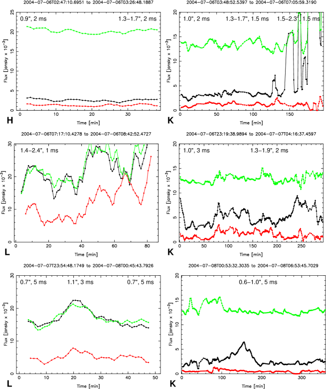
Figure 2: Light curves of all NIR observations in July 2004. Shown are the dereddened flux densities of S1 (green), Sgr A* (black), and a field free of stars (red). The data were smoothed with a sliding point window comprising five samples in case of the K- and H-band data, 9 samples in case of the L’-band data. Here, one sample corresponds to a photometric measurement on an individual image (i.e., DIT$\times$NDIT integration time, see Table 2). Filters are indicated in the lower left corners, start and stop times on top of the plots. As can be seen, the quality of the data is fairly variable. This is closely related to the seeing and coherence time of the atmosphere during the observations, which result in a variable performance of the AO system. We indicated seeing and atmospheric coherence time in the plots. If there is more than one label in a given plot, then the location of the labels indicates approximately the time window to which the seeing/coherence time values apply. For example, in the L’-band data, seeing and coherence time deteriorated continuously during the observations on July 06/07, while in the July 08 data, only a brief episode of bad seeing occurred near the end of the first third of the time series. Generally, the light curve of S1 and of the background, which are expected to be constant, give a good idea of the data quality and relative uncertainties of the observations. Values for seeing and coherence time were taken from the web site of the ESO Observatories Ambient Conditions Database.

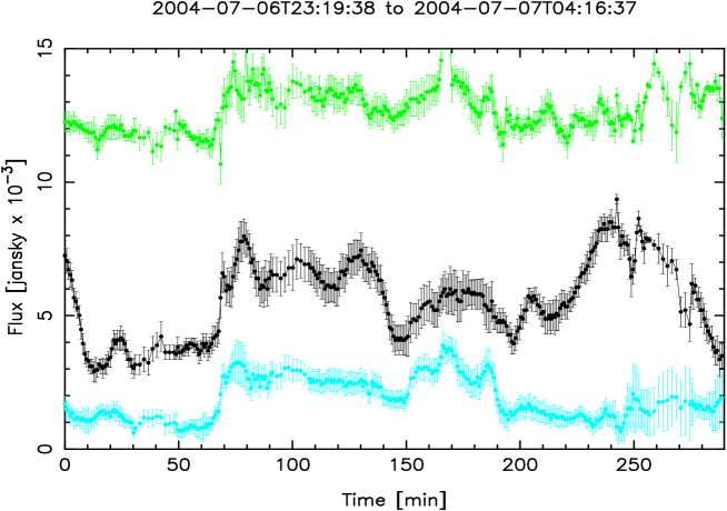
Figure 3: Light curve of the K-band observations from July 07 (see Fig. 2). The plot shows the lightcurves of S1 (top),SgrA* (middle), and the background flux (bottom).

The flux densities of the sources were measured by aperture photometry with circular apertures of 52 mas radius and corrected for extinction, using $A_{H}=4.3$, $A_{K}=2.8$, and $A_{L^{\prime}}=1.8$. Calibration of the photometry and astrometry was done with the help of the known fluxes and positions of 9 sources within $1.6"$ of Sgr A*. Uncertainties were obtained by comparing the results of the photometry on the LR and LIN deconvolved images. The background flux was obtained by averaging the measurements at five random locations in a field about $0.6"$ west of Sgr A* that is free of obvious stellar sources. The average positions and fluxes of Sgr A* obtained from the NIR observations are listed in Tab.3. Fig. 2 shows a plot of the flux versus time for Sgr A*, S1, and the background. As can be seen, the background is fairly variable. These background fluctuations are present in the light curves of Sgr A* and S1 as well, as can be seen in the Figure. It is therefore reasonable to subtract the background flux from the light curves. The result is shown in Fig. 3. The source S1 now shows an almost constant flux density as expected.

2.2 The Chandra X-ray Observations

In parallel to the NIR observations, SgrA* was observed with Chandra using the imaging array of the Advanced CCD Imaging Spectrometer (ACIS-I; Weisskopf et al., 2002) for two blocks of $\sim$50 ks on 05–07 July 2004 (UT). The start and stop times are listed in Table 1. The instrument was operated in timed exposure mode with detectors I0–3 turned on. The time between CCD frames was 3.141 s. The event data were telemetered in faint format.

We reduced and analyzed the data using CIAO v2.3 software with Chandra CALDB v2.22. Following Baganoff et al. (2003), we reprocessed the level 1 data to remove the 0.25″ randomization of event positions applied during standard pipeline processing and to retain events flagged as possible cosmic-ray after-glows, since the strong diffuse emission in the Galactic Center causes the algorithm to flag a significant fraction of genuine X-rays. The data were filtered on the standard ASCA grades. The background was stable throughout the observation, and there were no gaps in the telemetry.

The X-ray and optical positions of three Tycho-2 sources were correlated (Høg 2000) to register the ACIS field on the Hipparcos coordinate frame to an accuracy of 0.10″ (on axis); then we measured the position of the X-ray source at Sgr A*. The X-ray position [$\alpha$_J2000.0 = $17^{\mathrm{h}}45^{\mathrm{m}}40.030^{\mathrm{s}}$, $\delta$_J2000.0 = $-29\mbox{${}^{\circ}$}00\arcmin 28.23\arcsec$] is consistent with the radio position of Sgr A* (Reid et al. 1999) to within $0.18\arcsec\ \pm 0.18\arcsec$ ($1\,\sigma$).

We extracted counts within radii of 0.5″, 1.0″, and 1.5″ around Sgr A* in the 2–8 keV band. Background counts were extracted from an annulus around Sgr A* with inner and outer radii of 2″ and 10″, respectively, excluding regions around discrete sources and bright structures (Baganoff et al. 2003). The mean (total) count rates within the inner radius subdivided into the peak count rates during a flare and the corresponding IQ-values are listed in Table 4. The background rates have been scaled to the area of the source region. We note that the mean source rate in the 1.5″ aperture is consistent with the mean quiescent source rates from previous observations (Baganoff et al. 2001, Baganoff et al. 2003). The PSF encircled energy within each aperture increases from $\approx 50\%$ for the smallest radius to $\approx 90\%$ for the largest, while the estimated fraction of counts from the background increases with radius from $\approx 5\%$ to $\approx 11\%$. Thus, the 1.0″ aperture provides the best compromise between maximizing source signal and rejecting background.

2.3 The VISIR MIR Observations

VISIR is the ESO mid-infrared combined imaging camera and spectrograph. The camera is located at the Cassegrain focus of UT3 (Melipal). It operates over a wavelength range of 8-13 and 17-24 $\mu$m with fully reflective optics and two Si:As Blocked Impurity Band (BIB) array detectors from DRS Technologies. These detectors provide 256$\times$256 elements with a pixel scale of 0.075 arcsec/pixel for the 8-13$\mu$m wavelength range and 0.127 arcsec/pixel for 17-24$\mu$m, resulting in fields of view of 19.2”$\times$19.2” and 32.3”$\times$32.2”, respectively. The operating temperature is 15K and the detector temperature lies below 7K. Background subtraction is performed via chopping and nodding. The filter wheel is located just behind the cold stop pupil and may hold up to 40 filters.

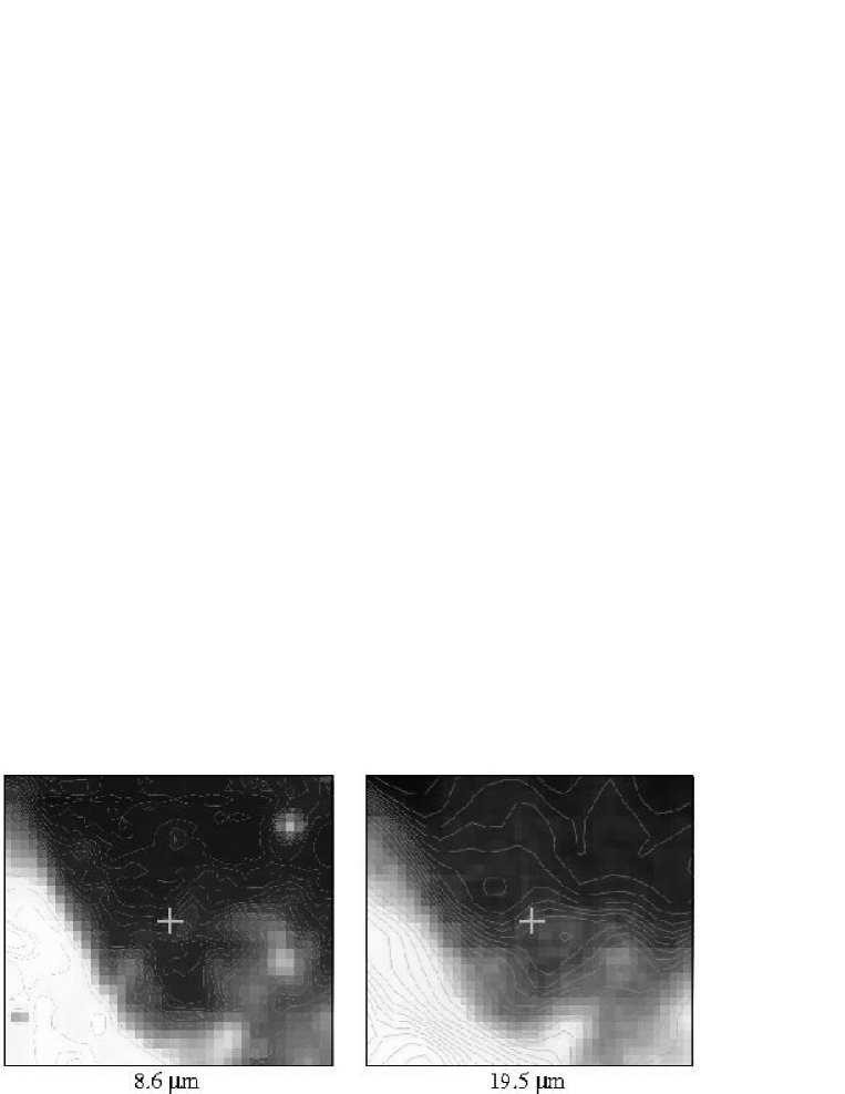
Figure 4: The 8.6$\mu$m (left) and 19.5$\mu$m (right) image of the central $5.0^{\prime\prime}\times 4.4^{\prime\prime}$ as taken with VISIR on 8 May 2004. The emission at the position of SgrA* is consistent with dust emission similar to what is measured towards other faint components within the central 5-10 arcseconds. The cross marks the position of SgrA* and the positional uncertainty of $\pm 0.2^{\prime\prime}$. As reference sources to determine the relative positioning between the NIR and MIR frame we used the bright and compact sources IRS 3, 7, 21, 10W and, in addition at 8.6$\mu$m wavelength, IRS 9, 6E, and 29.

The 8.6 $\mu$m and 19.5$\mu$m imaging data were taken on May 8, 9 and 10 (2004) as part of the instrument commissioning. For the images used here, the larger scale of 0.127″/pixel was used. The angular resolution was of the order 0.3-0.4” at 8.6$\mu$m and 0.6” at 19.5$\mu$m as measured from compact sources on the frames (e.g. IRS7). The images each comprise the average of typically seven chopped and flat-fielded exposures, with a typical integration time of 14 s (Fig. 4). Flux densities at the position of Sgr A* and the S-cluster (combined, due to the resolution of 0.3-0.4”) were extracted from these images, using IRS 21 as a flux calibrator. Tanner et al. (2002) report 8.8 $\mu$m flux densities of 1.34 Jy (1″aperture, background subtracted), 3.21 Jy (1″aperture, non-background-subtracted) and 3.6 Jy (2″aperture, non-subtracted) for this source. After adjusting for the different wavelength used (both wavelengths lie on the flank of the 9.7 $\mu$m silicate absorption feature, c.f. Lutz et al. 1996), we obtain a background-subtracted flux density of 5.11 Jy for IRS 21 in a 2″aperture. These flux densities also agree well with the 8.7 $\mu$m flux densities for the bright IRS sources measured by Stolovy et al. (1996), who found 5.6 Jy for IRS 21 (2″aperture, background not subtracted). Recent results (Scoville et el. 2003, Viehmann et al. 2005) suggest a lower extinction than the traditionally used $A_{V}$=27-30 magnitudes towards the Galactic Center. Consequently, we adopt $A_{V}$=25 magnitudes and thus $A_{\mathrm{8.6\mu m}}$=1.75 following the extinction law of Lutz et al. (1996), which results in an extinction-corrected flux density of 4.56 Jy for IRS 21 at 8.6 $\mu$m in a 1” aperture, which we used for calibration. The final flux density values at the position of SgrA* were obtained in a 1” diameter aperture. As reference sources to determine the relative positioning between the NIR and MIR frames we used the bright and compact sources IRS 3, 7, 21, 10W and in addition at 8.6$\mu$m wavelength IRS 9, 6E, and 29. As a final positional uncertainty we obtain $\pm 0.2^{\prime\prime}$. At both wavelengths the flux density is dominated by an extended source centered about 0.2”-0.3” west of SgrA*. This source was also noted by Stolovy et al (1996).

In Tab. 5 we list the flux densities obtained for the available 0.3-0.4” angular resolution VISIR data. We find a mean flux density of 30$\pm$10 mJy (1$\sigma$) at 8.6$\mu$m wavelength with a tendency for larger flux density values during times of poorer seeing. The differences are also mainly between data sets taken at different days. There are no signs of a strong (i.e. several $\sigma$) deviation. We adopt a dereddened flux density at 8.6$\mu$m wavelength of 50 mJy as a safe upper limit. Following the same calibration procedure, assuming $A_{V}$=25, $A_{\mathrm{8.6\mu m}}$=1.75 and using 20.8$\mu$m flux densities for IRS 21 from Tanner et al. (2002), we find a flux density of 320$\pm$80 mJy at 19.5$\mu$m in a 1” diameter aperture at the position of SgrA*.

2.4 The SMA Observations

The Submillimeter Array observations of SgrA* were made at 890 $\mu$m for three consecutive nights, 05-07 July 2004 (UT), with the latter two nights timed to coincide with the Chandra observing periods. These observations were made with the Submillimeter Array (SMA), an interferometer operating from 1.3 mm to 450 $\mu$m on Mauna Kea, Hawaii (Ho, Moran, & Lo 2004). On both July 6 and 7 we obtained more than 6 hours of simultaneous X-ray/submillimeter coverage (Table 1); however, the longitudinal separation (nearly 90^∘) between the VLT and the SMA limits the period of combined IR/X-ray/submillimeter coverage to approximately 2.5 hours. The weather degraded over the course of the three nights, from a zenith opacity at 890 $\mu$m of 0.11 on July 5 to 0.15 and 0.29 on July 6 and 7, respectively. This is reflected in the larger time bins and scatter in the later light curves.

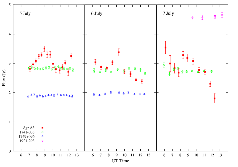
Figure 5: The 890 $\mu$m light curves from July 05-07. The light curves of the quasar calibrators, 1741$-$038, 1749$+$096, and 1921$-$293, are also shown. For each source we plot Stokes I, the total intensity. Due to poorer weather on July 06 and 07, for these days we have averaged two cycles between SgrA* and the quasar calibrators (see text) for each data point, while the July 05 data is shown at full time resolution.

The SgrA* observations were obtained as part of an ongoing SMA study of the submillimeter polarization of this source (Marrone et al., in preparation). Because these observations are obtained with circularly polarized feeds, rather than the linearly polarized feeds usually employed at these wavelengths, these data do not have the ambiguity between total intensity variations and modulation from linear polarization that afflict previous (sub)millimeter monitoring (e.g. Zhao et al. 2003). This technique does mix the total intensity with the source circular polarization, but measurements at 1.3 mm (Bower et al. 2003, 2005) show no reliable circular polarization at the percent level. In SMA polarimetric observations, only one out of every 16 consecutive integrations on SgrA* is obtained with all antennas observing the same polarization (left or right circular) simultaneously, while the remaining integrations sample a combination of aligned and crossed polarizations on each baseline. For the light curves presented here (Figure 5) we use only the 50% of integrations on each baseline obtained with both antennas in the same polarization state, as cross-polar integrations sample the linear polarization rather than the total intensity. This unusual time sampling should not affect the resulting light curves, as each point is an average of at least one 16 integration cycle. Nearby quasars were used for phase and gain calibration. On July 5 and 6, the observing cycle was 3.5 minutes on each of two quasars (1741$-$038, 1749$+$096), followed by 14 minutes on SgrA*. On July 7 we used a shorter cycle and stronger quasars in the poorer weather, 3.5 minutes on either 1741$-$038 or 1921$-$293 followed by 7 minutes on SgrA*, with the two quasars interleaved near the end of the observations. Although 7 or 8 antennas were used in each track, only the same 5 antennas with the best gain stability were used to form light curves, resulting in a typical synthesized beam of 1$\aas@@fstack{\prime\prime}$5$\times$3$\aas@@fstack{\prime\prime}$0. The poor performance of the other antennas can most likely be attributed to pointing errors. We were concerned about the effects of changing spatial sampling of smooth extended emission on the flux densities we obtain from subsets of our SgrA* observation. Images of the full three-day data set show very little emission away from SgrA*, with peak emission around 3% of the amplitude of the central point source. To reduce sensitivity to the largest angular scales we sample, we have excluded the two baselines that project to less than 24 k$\lambda$ (angular scales $>$9″) during the SgrA* observations. A comparison of the variations in the three daily light curves versus hour angle shows no conclusive common variations above the 10% level, but the presence of differential variations of 30% or larger will mask smaller systematic changes. We conclude that the surrounding emission is not responsible for changes larger than around 10%, and may in fact be significantly less important.

The SgrA* data is phase self-calibrated after the application of the quasar gains to remove short-timescale phase variations, then imaged and cleaned. Finally, the flux density is extracted from a point source fit at the center of the image, with the error taken from the noise in the residual image. The overall flux scale is set by observations of Neptune, with an uncertainty of approximately 25%. The complete data sets from each night, including other quasar observations not used in this analysis, show some systematic day-to-day flux variations across sources at the 15% level. These have been removed here by assuming that the mean of the quasar flux densities remain constant from day to day. Because we have used multiple sources to remove this inter-day variation, we believe this part of the absolute calibration to be accurate to about 10%. Nevertheless, these uncertainties do not affect the errors within each day’s light curve.

2.5 The VLA 7 mm Observations

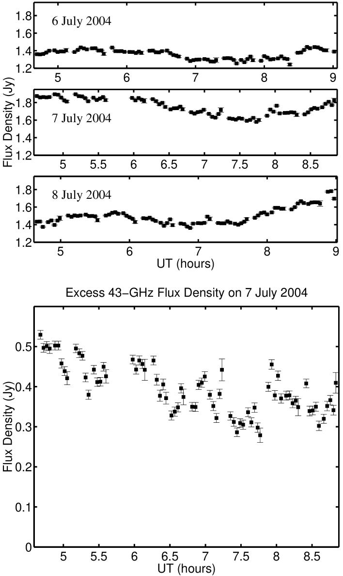
Figure 8: VLA 43 GHz light curves. The top graphs show the correlated flux density as measured on 6, 7, and 8 of July (see Tab. 1). The bottom graph shows the excess flux density on 7 July calculated as the difference between the data from this day and the mean of 6 and 8 July.

The Very Large Array (VLA) observed Sgr A* for $\sim 5$ hours on 6, 7 and 8 July 2004. Observations covered roughly the UT time range 04:40 to 09:00 (see also Table 1), which is a subset of the Chandra observing time on 6 and 7 July. Observations on 6 July also overlapped with NIR observations. The VLA was in D configuration and achieved a resolution of $2.5\times 0.9$ arcsec at the observing wavelength of 0.7 cm. Fast-switching was employed to eliminate short-term atmospheric phase fluctuations and provide accurate short-term amplitude calibration. For every 1.5 minutes on Sgr A*, 1 minute was spent on the nearby calibrator J1744-312. Antenna-based amplitude and phase gain solutions were obtained through self-calibration of J1744-312 assuming a constant flux density. Absolute amplitude calibration was set by observations of 3C 286. Flux densities were determined for Sgr A* and J1744-312 through fitting of visibilities at $(u,v)$ distances greater than 50 $k\lambda$. This $(u,v)$-cutoff removed contamination from extended structure in the Galactic Center. We simultaneously fit for the flux density of the two components of a transient source 2.7 arcsec South of Sgr A* (Bower et al. 2005). The corresponding light curves of SgrA* for 6, 7 and 8 July 2004 are shown in Fig. 8 (see also Table 1).

3 Properties of the Light Curves

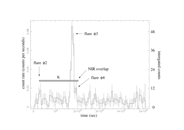
Figure 6: Chandra light curve for 6/7 July 2005. We also indicate the overlap with the NIR data. Start time is 2004 July 6, 22:35:11.8; Stop time is 2004 July 7, 12:53:44.9.

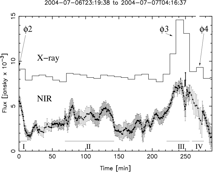
Figure 9: The X-ray and NIR light curves plotted with a common time axis. See text and captions of previous figures. Straight solid lines in the inserted box represent the 0.00, 0.01, and 0.02 counts per second levels. The straight dashed line represent the X-ray IQ-state flux density level.

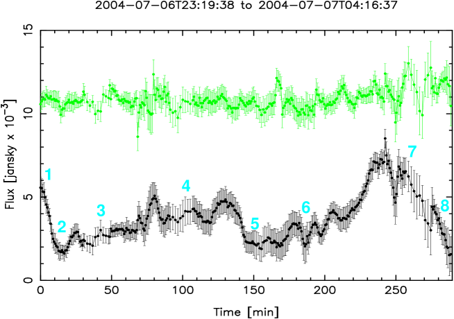
Figure 10: Light curve of the K-band observations from July 07 (see Fig. 2). The plot shows the lightcurves of S1 (top) and SgrA* (bottom). From both plots we have subtracted the background level. The numbers near the light curve of Sgr A* mark the approximate time points for which images are shown in Figure 11.

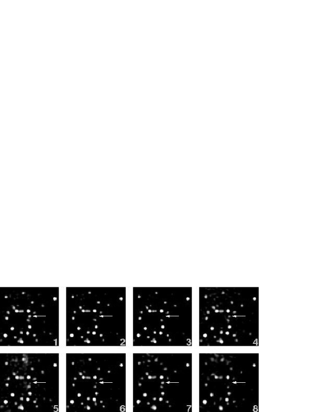
Figure 11: K-band images of the stellar cluster in the immediate vicinity of Sgr A*. The numbers correspond to the time points indicated in Figure 10. The images result from the average of five individual exposures, corresponding to 150 s total integration time. A LR deconvolution and restoration with a Gaussian beam was applied. The color scale is linear. North is up, east to the left. The offsets are given with respect to the position of SgrA*. The white arrows indicate the position of Sgr A*.

The light curves show several flare events. In the following we base the identification of individual flares on their significant detection in at least one of the observed wavelength bands. We have significant detections of a total of 5 NIR flare events (labeled I - V in Tab. 6 see also Fig.9) and one bright X-ray flare (labeled $\phi$3 in Tab. 4 see also Fig. 6). For 4 of the 5 NIR events we have simultaneous data coverage in both wavelength domains. In Figures 3 and 10, the light curve of the K-band imaging from 7 July is shown separately. Four NIR bursts (I - IV) can be seen. All of them were covered by simultaneous Chandra observations. In Fig. 11, images corresponding to the time points marked in Fig. 10 are shown. The images show the “on” and “off” states of Sgr A*.

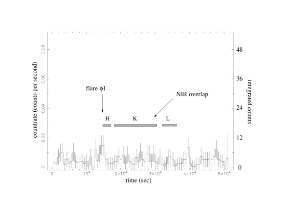
Figure 7: Chandra light curve for 5/6 July 2005. We also indicate the overlap with the NIR data. Start time is 2004 July 5, 22:38:25.7; Stop time is 2004 July 6, 12:56:58.8.

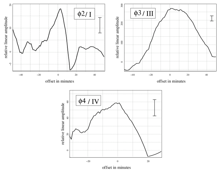
Figure 12: Cross-correlation between the NIR data (40 second bins; 20 seconds integration time per image) and the X-ray data (10 minute bins) for the three flares $\phi$2/I (top left), $\phi 3$/III (top right), and $\phi 4$/IV (bottom; see Tab.7). We cross-correlated only the flare data that overlap in time i.e. about 40 minutes before and 20 minutes after midnight 07 July 0.0 UT for flare $\phi$2/I, about 177 minutes until 223 minutes after midnight for $\phi 3$/III, and about 223 minutes until 256 minutes after midnight for $\phi 4$/IV. The error bars indicate an estimate of the SNR derived from the SNR of the individual X-ray bins and the approximate number of bins that were averaged for each of the cross-correlations measurements. At a $\sim$2.6, 9, and 3$\sigma$ level, respectively, the light curves indicate a simultaneous flare event around midnight corresponding to a time delay of less than 10 minutes (see text). For flares $\phi 3$/II and $\phi 4$/IV the entire event was covered. The offsets are given in minutes.

In the X-ray regime we also draw attention to the weak flux density increases labeled $\phi$2 and $\phi$4 in Tab. 4 (see also Fig. 7) which coincide with significant NIR flares (labeled I and IV in Tab. 6 and Fig. 6), and to one weak X-ray flux density increase $\phi$1 which is similar to $\phi$2. In the following we consider these as weak flare candidates. The interest in the weak events $\phi$2 and $\phi$4 is strengthened by the cross-correlation with the corresponding NIR flares (see Fig. 12). Fig. 7 shows that the weak X-ray flare $\phi$1 did not have a detectable H-band counterpart. The H-band observations started almost exactly at the time of the peak X-ray emission. As shown in Fig. 6 the candidate (but insignificant by itself) weak X-ray flare $\phi$2 was covered by NIR K-band measurements starting at its X-ray peak emission covering the decaying part of the event. The excursion in the count rate labeled $\phi$2 (which is insignificant by itself) occurs simultaneous to the significant NIR event II, which justifies its discussion. The moderately bright X-ray flares $\phi$3 and $\phi$4 were fully covered in the NIR domain as well (see Figs. 6 and 9). Flare $\phi$4 follows immediately after $\phi$3 and is similar in total strength and spectral index to $\phi$2. The cross-correlation (Fig. 12) between the X-ray and NIR flare emission results in an upper limit for a time lag between both events of about 10 minutes. The graph shows a clear maximum close to 0 minutes delay indicating that within the binning sizes both data sets are well correlated. Between the X-ray/NIR flares $\phi$2/I and $\phi$3/III we detect a lower level NIR flare phase which has no significant counterpart in the X-ray domain. Finally the NIR flare V (see Figs. 2 lower, right corner) was not covered by our X-ray data. In Tab. 7 we give a summary of the observed flux densities and spectral indices of all considered events.

We can estimate the times at which the flare emission was negligible, i.e. equal to the low level variability IQ-state emission in the X-ray and NIR domain. The corresponding full width at zero power (FWZP) and FWHM start and stop times are given in Tabs. 4 and 6. For the weak candidate flare events $\phi$1, $\phi$2, and $\phi$4 we only give estimates of FWZP. In summary the statistical analysis of the combined X-ray and NIR data for the 2004 observations shows that SgrA* underwent at least one significant flare event simultaneously in both wavelength regimes.

The 890$\mu$m SMA submillimeter light curve (Figure 5) does not show an obvious constant flux level, but instead is continuously varying (as it is probably the case for the NIR emission as well). Several flux density excursions of $10-20$% are visible over the three observing nights; the variations typically occur on $1-2$ hour timescales, although there are also abrupt changes, such as the drop around 09:30 UT on July 6 (SMA 3 in Tab. 8). These slow variations occur on somewhat longer timescales than the X-ray and IR variations, perhaps suggesting that the 890 $\mu$m emission extends out to regions tens of Schwarzschild radii away, where causality slows the observed changes in the total flux density integrated over the whole source. However, measurements at 7 mm by Bower et al. (2004) suggest that the source is only 20$-$30 R_s in diameter, corresponding to only about 10 minutes of light travel time, so these slow variations are probably not due to propagation effects.

The only period of coincident observations in the IR and submillimeter, 2.5 hours on July 6, is rather featureless in the submillimeter. Unfortunately, this portion of the IR observations is not very reliable because very short atmospheric coherence times resulted in poor AO performance (see Figure 2, upper right from minute 134 onward, and middle left).

A comparison of the sub-millimeter and X-ray light curves shows that on July 7 the decaying 43 GHz excess is accompanied by a $\sim$1 Jy sub-millimeter flux density decay (SMA 4 in Tab. 8). After a small increase by about 0.5 Jy (SMA 5 in Tab. 8) that decay continues over the entire observing period on 7 July (see red squares in the right panel of Fig.5) and amounts to a total decrease in flux density of about 2 Jy. As the observing interval started about 2.3h after the X-ray flare $\phi$3 and NIR flare III we speculate in section 7.1 that the sub-millimeter decay may be linked to adiabatic expansion of the emitting plasma.

Furthermore the comparison with the X-ray light curve shows that one prominent submillimeter feature, a slow rise over 1.5 hours punctuated by a sharp drop in flux density at 09:30 UT on July 6, (SMA 3 in Tab. 8) is coincident with a very small increase in the X-ray flux at 39.4 ks in Figure 7. This may be evidence that flares observed at shorter wavelengths can be foretold by a slow rise in submillimeter emission. This slow rise could manifest itself best in the submillimeter if the IR and X-ray are dominated by SSC emission, which varies non-linearly with the synchrotron emission. However, this increase in the X-ray count rate is not very statistically significant.

The 7 mm VLA radio light curves show relatively small variations on 6 and 8 July with characteristic amplitudes of $\sim 10\%$. On July 7, however, the flux density starts higher than on the previous day by about 0.5 Jy, or $\sim 40\%$ of the mean flux density on July 6 (Tab. 8). The flux density declines steadily over the next three hours, reaching a minimum of 1.6 Jy. The mean flux density on July 7 is $\sim$0.4 Jy in excess of the average flux density on July 6 and 8. The July 7 observations covered the time interval about 1.5 to 5 hours after the the peak of X-ray flare $\phi$3 i.e. NIR flare III. Given the lack of simultaneous radio observations with the flare peak we can only guess at the detailed relationship between the rise in the radio flux density and the X-ray/NIR flare (see section 7.1). We cannot constrain whether the radio flux density rise precedes or follows the X-ray flare, or, for that matter, whether it is related to an X-ray flare that may have occurred during the 10 hours between the two Chandra observations.

4 NIR to X-Ray Flux Densities and Broad Band Spectral Indices

Consistent with previous Chandra observations (Baganoff et al. 2001, 2003, Eckart et al. 2004) the IQ-state X-ray count rate in a 1.5” radius aperture during the monitoring period is $5.3\pm 0.5\times$10^-3 counts s^-1. This corresponds to a 2 - 8 keV luminosity of 2.2$\times$10³³ erg/s or a flux density of $0.015\mathrm{\mu}$Jy. The excess X-ray flux density observed during the strongest simultaneous flare event $\phi$3 was 0.223$\pm$27 $\mu$Jy. This is about a factor of 15 higher than the IQ-state and corresponds to a 2 - 8 keV luminosity of about 33$\times$10³³ erg/s. For the other three events $\phi$1, $\phi$2, and $\phi$4 the excess was only a factor of 1.5 to 2 above the flux of the -state. In the infrared the $2.2\mathrm{\mu}$m extinction corrected flux density of the low level variability IQ-state Sgr A* counterpart was found to be of the order of $3$ mJy and the excess flux density observed during the flares was only of the order of $5$ mJy.

For the stronger flare $\phi$3 we find a spectral index of $\alpha_{X/NIR}$$\sim$1.12 (with $S_{\nu}$$\propto$$\nu^{-\alpha}$) between the NIR regime (here at a wavelength of $2.2\mathrm{\mu}$m) and the X-ray domain (here centered approximately at an energy of 4 keV). For the three weaker flares ($\phi$1, $\phi$2, and $\phi$4) we find $\alpha_{X/NIR}$$\sim$1.35, comparable to the value given for the event reported by Eckart et al. (2004) (see also Tab.7). This shows that the amplitude range of the X-ray flare emission is larger than that observed in the infrared and that the infrared and X-ray flare strengths are not necessarily proportional to each other. It also suggests that stronger flare events may have a flatter overall spectrum. The fact that the NIR spectral indices measured by Eisenhauer et al. (2005) and Ghez et al. (2005) are usually much steeper than the overall X-ray/NIR spectral indices is discussed in detail in section 7.

5 The MIR/NIR Spectrum of SgrA*

5.1 The NIR Spectrum of SgrA*

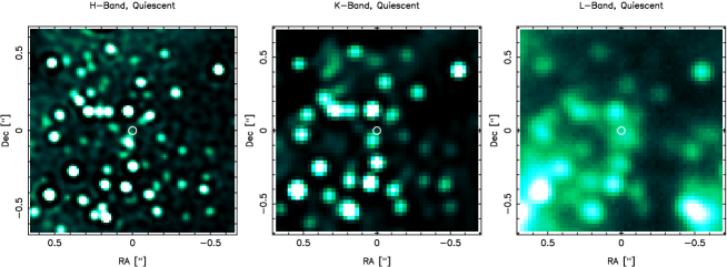
Figure 13: Images of the stellar cluster in the immediate vicinity of the center during the IQ, low NIR flux density state of Sgr A*. The images result from the average of several individual exposures, corresponding to a total integration time of 40 minutes for H-band, 100 minutes for K-band, and 80 minutes for L’-band. LR deconvolution and restoration with a Gaussian beam was applied. The color scale is linear. North is up, east to the left. The field of view shown in each image is $1.3^{\prime\prime}\times 1.3^{\prime\prime}$. The white circles indicate the position of Sgr A*. All images were taken on the 6 July 2004. The positional accuracy of the images is of the order of 0.5 pixels, i.e. $\sim$7 mas in the H-band and $\sim$14 mas in the K- and L’-bands.

On July 6 we covered the central region in the NIR H-, K-, and L’-band with no detectable NIR flare emission during a quiescent period with the exception of a short and weak decaying X-ray flare at the beginning of our H-band exposure (NIR flare event I in Tab. 6). In Fig. 13 we show the corresponding images during this phase in all three NIR bands (H-, K-, and L’-band). These images show that very little emission originates from potential sources at the position of SgrA*. Both at H- and K-band the flux density may be severely influenced or even dominated by emission due to the stellar background.

The NIR spectral energy distribution of the flaring states of SgrA* appears to be very red. Using the new integral field spectrometer SINFONI at the VLT, Eisenhauer et al. (2005) obtained simultaneous NIR spectral energy distributions ($\nu$L_ν=$\nu^{-\epsilon}$) of three flares. They find that the slopes vary and have values ranging from $\epsilon$=2.2$\pm$0.3 to $\epsilon$=3.7$\pm$0.9 during weak flares of SgrA*. This corresponds to a spectral index $S_{\nu}$$\propto$$\nu^{-\alpha}$ range of about $\alpha$=3-5. Here we assume that their subtraction of spectral data cubes before the flare events did only correct for scattered light/spillover and foreground/background stellar emission along the line of sight toward SgrA* and that the possible contribution of the flare emission to the flux density obtained at these times before the flare event is negligible. Under these circumstances the differential spectral shapes can be regarded as true spectra of the NIR flares.

In recent narrow band measurements with the Keck telescope Ghez et al. (Ghez et al. 2005, and private communication) also found a red intrinsic flare spectrum. These measurements, however, indicate a considerably flatter spectrum with a slope of $\alpha$=0.5$\pm$0.3.

5.2 Contamination by MIR Dust Emission

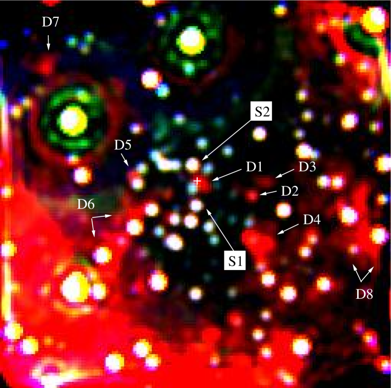
Figure 14: HKL’ multi-color image of the central $2.6^{\prime\prime}\times 2.6^{\prime\prime}$ as taken with NACO on 6 July 2004. North is up and East is to the left. H is blue, K is green, and L’ is red. The white cross marks the position of SgrA*. The figure is a different representation of the same data shown in Fig. 13 covering a larger field of view. Just west of the position of SgrA* an extended red emission component D1 is evident.

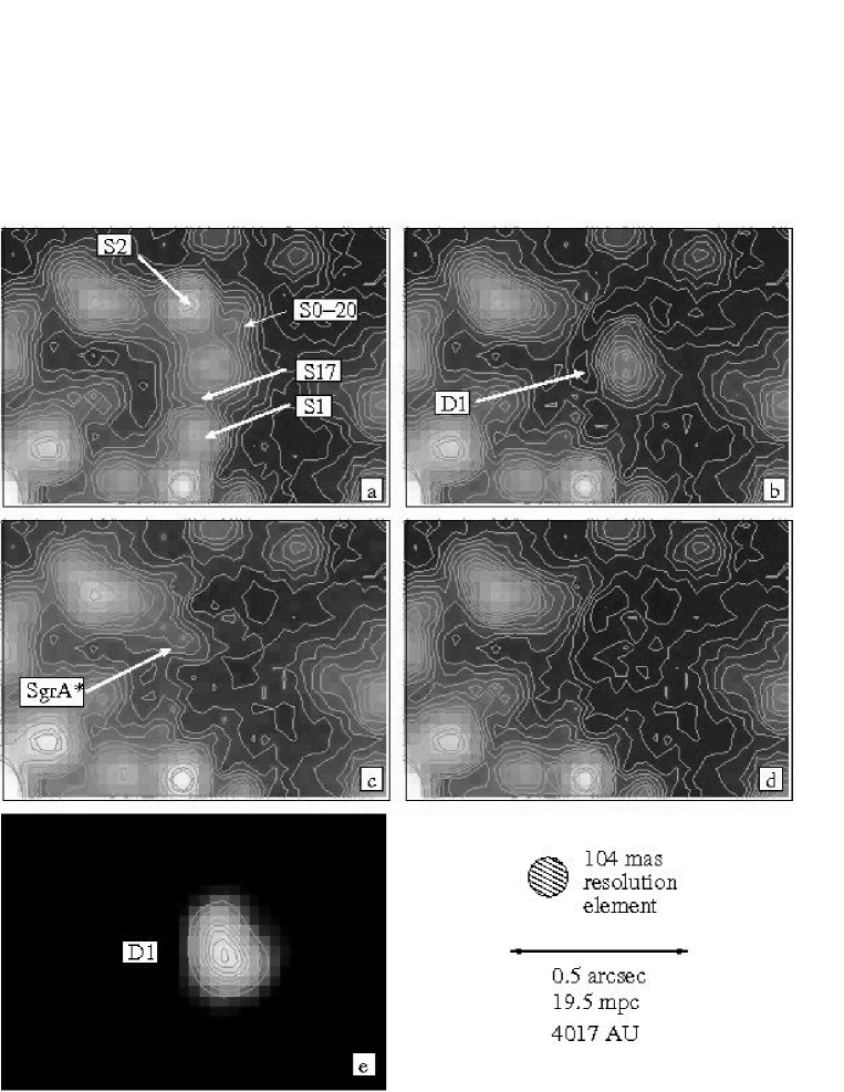
Figure 15: The central 0.76”$\times$1.06” shown in a color and contour map. The contour lines are 4, 6, 8, 10, 12, 14, 16, 18, 20, 22, 24, 26, 30, 35, 40, 42 10, 14, 19, 24, 29, 33, 38, 43, 48, 52, 57, 62, 71, 83, 95, 98 % of the peak brightness of star S2. Panel a) shows the complete L’ band images section. Panel b) shows the images section with scaled PSF subtractions of the sources S2 (L’=12.78 used as a calibrator), S1 (L’=13.80$\pm$0.12), S17 (L’=13.79$\pm$0.12), S0-20 (L’=13.89$\pm$0.13), and SgrA* (L’=14.1$\pm$0.2). The dust component D1 (L’=12.8$\pm$0.20) is clearly visible. Panel c) shows the images with D1 subtracted instead of SgrA*. In panel d) both SgrA* and D1 have been subtracted. Panel e) shows the model of the dust component D1 by itself. The background in the central 0.3” is flat and has a L’ brightness of L’=15 per beam with a 3$\sigma$ deviation of less than $\pm$0.42 magnitudes.

The images at wavelengths longer than 2.2$\mu$m show the existence of a flux density contribution from a weak and extended source D1 with a separation ranging between $\sim$30 mas and $\sim$150 mas from SgrA* (i.e. 80$\pm$50$mas$) (see Fig. 14 and 4; see also Ghez et al. 2004b, 2005). The FWHM diameter of the source D1 is of the order of 1400 AU at the distance of 8 kpc. In addition to the overall contribution of the mini-spiral to the dust emission there are several other red features of this kind labeled D2 to D8 in Fig. 14 within the central 2.6”$\times$2.6” region. At 8.6$\mu$m source D1 appears to be part of a larger ridge structure (tracing lower temperature dust; see also Stolovy, Hayward, & Herter 1996) at a position angle similar to a feature along an extension of dust emission from the mini-spiral towards the central cluster of high velocity stars (Fig. 14). This ridge continues further to the northwest and we interpret this emission component close to SgrA* as part of this extension. If this interpretation is correct then this component is probably due to continuum emission of warm dust. Deriving the flux density of this extended source D1 is difficult, as it is located in a crowded field and confused with the L’-band counterpart of SgrA*. Using an L’-band magnitude of $m_{L^{\prime}}$=12.78 for S2 (Ghez et al. 2005, Clenet et al. 2005) and following the approach of Ghez et al. (2005) of subtracting all neighboring point sources, we can confirm the location, extent, and overall shape of this extended component (Fig. 15). Since no activity of SgrA* was indicated by the H and K band exposures before and the X-ray exposure during the L’-band imaging on July 6 (see Tab.1) it is likely that SgrA* was in a low state. On July 6 we find for SgrA* $m_{L^{\prime}}$=14.1$\pm$0.2 (about 3.7 mJy dereddened), which is about half a magnitude brighter than what is reported by Ghez et al. (2005). This is consistent with SgrA* having been in a low flux density state during the L’-band exposure. We also find that within the uncertainties (in subtracting the neighboring sources including SgrA*) our data is consistent with an integrated L’-band magnitude of $m_{L^{\prime}}$$\sim$12.8 for the extended dust component, about 0.9 magnitudes brighter than what is given by Ghez et al. (2005), i.e. the extended source D1 is almost as bright as star S2. This would be consistent with a structure that is extended on scales larger (see L’ band magnitudes given in caption of Fig. 15) than 100 mas, to which the VLT AO telescope beam couples slightly better than the Keck beam. A brightness of m${}_{L}^{\prime}$=12.8$\pm$0.2 corresponds to a dereddened (m_ext=1.8) flux density of about 12$\pm$3mJy.

If the extended component D1 is associated with a gas and dust feature of the Galactic Center ISM then the 8.6$\mu$m flux density limit is very likely contaminated by emission from this extended dust feature as well. Assuming that this feature is not associated with SgrA* and has physical properties similar to the other dust emission components in the central parsec, we can determine its contribution to the 8.6$\mu$m emission. This can be approximated using its flux density value obtained in the L’-band and a mean flux density ratio between 8.6$\mu$m and 3.8$\mu$m obtained for the $\sim$200-400 K warm dust (Cotera et al. 1999). From our available L’- and N-band images we derive this flux density ratio of about 3 on individual warmer sources (like IRS 21) and about 12$\pm$4 on the overall region (derived from our data and consistent with the ISO spectrum shown by Lutz et al. 1996) which is dominated by the flux density contribution of the extended mini-spiral. Hence we find from the L’-band flux density estimate of this component that within the uncertainties it can easily account for most of the 8.6$\mu$m flux density at the position of SgrA*. Similarly on the mini-spiral we measure a flux density ratio between 19.5$\mu$m and 8.6$\mu$m of about 7$\pm$2 (consistent with Lutz et al. 1996). With the flux densities obtained at the position of SgrA* at 8.6$\mu$m and 19.5$\mu$m the emission is consistent with being due to dust similar to that found in the mini-spiral.

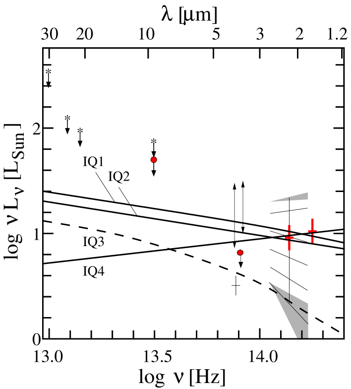
Figure 16: The NIR/MIR spectrum of SgrA* compared to emission models during low flux density states. Red data points indicate the measurements described in this paper. The log($\nu$ L_ν) values are based on the following data: Our new quasi-simultaneous L’-, K-, and H-band flux densities during the low NIR flux IQ-state are shown in red. The 30$\mu$m and 24.3$\mu$m flux density limits are taken from Telesco et al. (1996 APJ 456,541) and Serabyn et al. (1997), respectively; at 8.7$\mu$m our limit of about 100 mJy is lower than the value given by Stolovy et al. (1996); at 3.8$\mu$m our IQ flux density value (19$\pm$5 mJy) and the IQ flux density values (6.4 - 17.5 mJy) given by Genzel et al. (2003) as well as the range of flux densities (4 - 17 mJy, 1.3$\pm$0.3 mJy) given by Ghez et al. (2004, 2005). For clarity we displaced the latter two ranges slightly in frequency with respect to the center of the L’-band. In addition we plot representative SSC models IQ1-IQ4 with parameters as listed in Tab. 9.

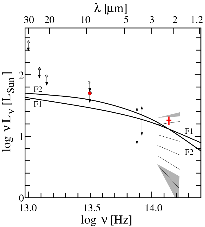
Figure 17: The NIR/MIR log($\nu$ L_ν) spectrum of SgrA* compared to flare emission models for the strong X-ray/NIR flare $\phi\leavevmode\nobreak\ 3/III$. See also caption of Fig. 11. Finally we show the K-band spectra of flares including the slopes (grey shaded area) as measured by Eisenhauer et al. (2005) and Ghez et al. (2005). The thin lines between the grey shaded areas indicate how the slope may change as a function of flare flux as suggested by Ghez et al. (2005). In addition we plot representative SSC flare models F1 and F2 with parameters as listed in Tab. 7.

In Figs.16 and 17 we show the flux densities or their limits towards SgrA* expressed via the energy output $\nu$L_ν as a function of frequency $\nu$. The plots cover the wavelength range between 30$\mu$m and 1.6$\mu$m. In the mid-infrared ($\lambda$$\geq$8.6$\mu$m) only flux density limits are available. For the NIR K-band we have plotted the envelope of the spectral data obtained by Eisenhauer et al. (2005) and Ghez et al. (2005). For the L’-band we compare our value of the low level variability IQ flux densities with the corresponding data intervals given by Genzel et al. (2003) and Ghez et al. (2004a, 2005) (see caption of Fig.16).

It is likely that the L’-band IQ state continuum emission obtained for SgrA* is also to a small extent effected by a contribution from the weak, extended emission component (see section 3 and Fig. 14 and 4. This contribution will depend critically on the aperture used and the location of the red emission component with respect to SgrA*. We estimate that for the high angular resolution L’-band images this contribution cannot be larger than a few mJy. For the 8.6$\mu$m band our flux density limit obtained from the VISIR commissioning data is lower than the (dereddened) value of $\sim$100 mJy derived by Stolovy et al. (1996). The values obtained by Telesco et al. (1996) and Serabyn et al. (1997) very likely include continuum emission contributions associated with dust components in the central parsec.

Extrapolating the SINFONI spectral slopes towards lower frequencies, their predicted flux densities lie within or above the quiescent state fluxes obtained in the L’-band by Genzel et al. (2003), Ghez et al. (2004a) and the value reported in this paper. Given that the data at longer wavelengths including those at 8.6$\mu$m only represent upper limits of the flux densities of SgrA*, the predicted values obtained by an extrapolation of the steep K-band spectra lie well above these limits and the expected intrinsic energy output of SgrA*. This is especially true if a flux density level equivalent to the quiescent state were to be added back to the flare spectroscopy data. Of course we do not know whether the MIR data have been taken during the low level flux density (IQ) or flare state and in principle it is possible that SgrA* becomes very bright in the MIR during a flare. However, SgrA* has been observed frequently during the past two decades and strong flare activity has never been reported at these wavelengths. In total the combination of the very steep flare spectra and the low flux density limits of SgrA* especially at 8.6$\mu$m and longward imply that the intrinsic spectral energy distribution of SgrA* flattens significantly for wavelengths longward of 4$\mu$m.

6 Flares in the NIR and X-Ray Domain

The durations of flares found in the observations presented here is in agreement with the current statistics. Baganoff et al. (2001), Eckart et al. (2004), and Porquet et al. (2003) report on X-ray events of 45 to 170 minutes. Eckart et al. (2004), Ghez et al. (2004a), and Genzel et al. (2003) report on NIR flare events that last 50 to 80 minutes, respectively. Simultaneous observations indicate that the NIR and X-ray flare events are well correlated in duration (see section 3). In the following we will assume as a working hypothesis that the activity of SgrA* consists of consecutive flare events of variable strength that have a characteristic duration of the order of 100 minutes. We further assume that flare event rate (the number of flares of a given strength per day) and flare event strength can be described by a power-law. Deviations from this assumption are discussed towards the end of this section.

From the statistics of such flares and the NIR flux density monitoring that was compiled over the past decade one can assume a power-law representation that allows us to predict the flare rate i.e. the number of flares of a given strength per day. We assume that the power-law will be truncated at both ends. At the high end this can be justified by the fact that flares much stronger than the neighboring high velocity S-stars have never been observed, and that the accretion process within a characteristic time scale must have a limited radiation efficiency. A truncation at the low end can be justified by the (currently) continuous supply of stellar wind material from the He-stars within the central 0.2 pc diameter of the stellar cluster.

Based on the measurements of 2003 the estimated infrared flaring rate is very high: 4 IR flare events were found within a total of 25 hours of observations, which results in about 2 to 6 events per day when assuming Poisson statistics (Genzel et al. 2003). With our most recent observations presented here we cover a total of 0.71 days and find 4 infrared flare events, 2 of which are above 5 mJy. We can therefore confirm the rate of NIR (mostly) K-band flares of 4$\pm$2 per day with a strength of approximately 10$\pm$5 mJy. This leaves us with the rate of flares weaker than about 5 mJy of 10.4$\pm$2 per day (the remainder of 24 h not covered by $>$5 mJy flares divided by the characteristic flare duration). Here we include the IQ state and assume that it can be represented by weak, consecutive flares of the same average length of 100 minutes.

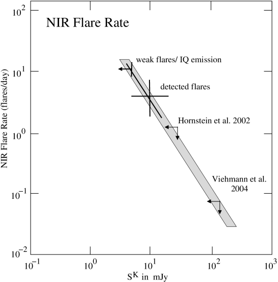
Figure 18: Flare amplitude as a function of flare rate for the NIR emission from SgrA* under the assumption that the characteristic flare duration is of the order of 100 minutes.

As for stronger flares, Hornstein et al. (2002) find from the analysis of Keck high angular resolution K-band imaging that the probability that a flare event of 3 hour duration has occurred with a flux density in excess of 19mJy is at most 9%. This corresponds to an equivalent flare rate of $\leq$0.7 events of 3 hour duration per 24 hours or $\leq$1.3 per day assuming a flare duration of 100 minutes. For the shorter duration we increase the detection flux level by $\sqrt{2}$ to 27m Jy. Performing a similar analysis for ISAAC data Viehmann et al. (2004) and Eckart et al. (2003) find a likelihood of 0.5% for 3 hour flares with a flux density of more than 100mJy. The equivalent flare rates are 3.6$\times$10^-2 for 3 hour flares and 7.2$\times$10^-2 for 100 minute flares per day. Similarly we increase the detection flux level by $\sqrt{2}$ to 141 mJy for the shorter assumed flare length of 100 minutes. In Fig. 18 we plot these quantities. The data can be described by a power-law of the form $N=\kappa_{0}(A)^{-\zeta}\kappa_{1}\kappa_{2}$. Here the quantities $\kappa_{0}$ and $N$ are in units of flare events per 24 hours, and $\kappa_{1}=exp(-\frac{A}{A_{high}})$ and $\kappa_{2}=exp(-\frac{A_{low}}{A})$ allow for a truncation of the power-law towards strong and weak flare events. $A_{high}$ and $A_{low}$ are cutoff flux densities at the high and low end of the power-law. Treating the limits as real measurements we find $\zeta$=-1.4$\pm$0.2 and $\kappa_{0}$=100$\pm$30. We note that in the case that our assumption that the flare length is independent of the flare amplitude has to be modified, one can make the following statements: If the overall characteristic flare duration is shorter or longer than 100 minutes then the power-law will be largely unaffected. It would still pass through the point given by the detected flares. Since the flare rate would be higher and the flare fluxes lower, changing the flare duration would correspond to a shift along the power-law line. If the flare duration is shorter only for weaker flares then the power-law can be extended towards the top. If stronger flares become longer their rate goes down resulting in a steeper slope of the power-law. Similarly if the flare duration is shorter for stronger flares then the slope will be shallower. An alternative to the truncated power-law representation that can currently not be ruled out is that the involved quantities like flare event rate, length, and strength are represented by peaked functions like a Gaussian.

It is highly improbable that the observed variability is due to stellar sources because of the extremely short time scales of the flares and because of the astrometric positions of the flares, which are within less than 10 mas of Sgr A* at all times (see also Tab. 3): a star close to Sgr A* would have moved by $\sim 20-50$ mas during the time interval covered by the four flares reported by Genzel et al. (2003). A star at greater distances from Sgr A* would have an extremely low probability of being located so close in projection to Sgr A*.

As for the relation between the NIR flares and variability in the X-ray domain, the durations, rise, and decay times are similar (see e.g. Baganoff et al. 2001, Porquet et al. 2003). The NIR flare rate, however, was almost twice as high as the X-ray flare rate during the Chandra monitoring in 2002. Also the range in spectral luminosities of the X-ray flares appears to be larger than in the NIR (including the brightest X-ray flares). X-ray flares a factor of $>$10 stronger than the quiescent emission occur at a rate of $0.53\pm 0.27$ per day, weaker flares are seen at a rate of $1.2\pm 0.4$ (Baganoff et al. 2003). Flares in the X-ray domain have been observed since 2000 (Baganoff et al. 2001, 2003, Eckart et al. 2003, 2004, Porquet et al. 2003) and since 2003 in the NIR domain (Genzel et al. 2003, Ghez at al. 2004a, Eckart et al. 2004). Consequently further simultaneous observations are needed to determine the relation between the X-ray and NIR flares.

7 Physical Interpretation

The new simultaneous X-ray/NIR flare detections of the SgrA* counterpart presented here support the finding by Eckart et al. (2004) that for the observed flare it is the same population of electrons that is responsible for both the IR and the X-ray emission. Due to the short flare duration the flare emission very likely originates from compact source components. The spectral energy distribution of SgrA* is currently explained by models that invoke radiatively inefficient accretion flow processes (RIAFs: Quataert 2003, Yuan et al. 2002, Yuan, Quataert, & Narayan 2003, 2004, including advection dominated accretion flows (ADAF): Narayan et al. 1995, convection dominated accretion flows (CDAF): Ball et al. 2001, Quataert & Gruzinov 2000, Narayan et al. 2002, Igumenshchev 2002, advection-dominated inflow-outflow solution (ADIOS): Blandford & Begelman 1999), jet models (Markoff et al. 2001), and Bondi-Hoyle models (Melia & Falcke 2001). Also combinations of models such as an accretion flow plus an outflow in form of a jet are considered (e.g. Yuan, Markoff, Falcke 2002).

7.1 Description and Properties of the SSC Model

Current models (Markoff et al. 2001, Yuan, Markoff, Falcke (2002), Yuan, Quataert, & Narayan 2003, 2004, Liu, Melia & Petrosian 2006) predict that during a flare a few percent of the electrons near the event horizon of the central black hole are accelerated. These models give a description of the entire electromagnetic spectrum of SgrA* from the radio to the X-ray domain. In contrast we limit our analysis to modeling the NIR to X-ray spectrum of the most compact source component at the location of SgrA*. We have employed a simple SSC model to describe the observed radio to X-ray properties of SgrA* using the nomenclature given by Gould (1979) and Marscher (1983). Inverse Compton scattering models provide an explanation for both the compact NIR and X-ray emission by up-scattering sub-mm-wavelength photons into these spectral domains. Such models are considered as a possibility in most of the recent modeling approaches and may provide important insights into some fundamental model requirements. The models do not explain the entire low frequency radio spectrum and IQ state X-ray emission. They give, however, a description of the compact IQ and flare emission originating from the immediate vicinity of the central black hole. A more detailed explanation is also given by Eckart et al. (2004).

We assume a synchrotron source of angular extent $\theta$. The source size is of the order of a few Schwarzschild radii R_s=2GM/c² with R_s$\sim$10¹⁰ $m$ for a 3.6$\times$10⁶M_⊙ black hole. One R_s then corresponds to an angular diameter of $\sim$8 $\mu$as at a distance to the Galactic Center of 8 kpc (Reid 1993, Eisenhauer et al. 2003). The emitting source becomes optically thick at a frequency $\nu_{m}$ with a flux density $S_{m}$, and has an optically thin spectral index $\alpha$ following the law $S_{\nu}$$\propto$$\nu^{-\alpha}$. This allows us to calculate the magnetic field strength $B$ and the inverse Compton scattered flux density $S_{SSC}$ as a function of the X-ray photon energy $E_{keV}$. The synchrotron self-Compton spectrum has the same spectral index as the synchrotron spectrum that is up-scattered i.e. $S_{SSC}$$\propto$$E_{keV}$^-α, and is valid within the limits $E_{min}$ and $E_{max}$ corresponding to the wavelengths $\lambda_{max}$ and $\lambda_{min}$ (see Marscher et al. 1983 for further details). We find that Lorentz factors $\gamma_{e}$ for the emitting electrons of the order of typically 10³ are required to produce a sufficient SSC flux in the observed X-ray domain. A possible relativistic bulk motion of the emitting source results in a Doppler boosting factor $\delta$=$\Gamma$^-1(1-$\beta$cos$\phi$)^-1. Here $\phi$ is the angle of the velocity vector to the line of sight, $\beta$ the velocity $v$ in units of the speed of light $c$, and Lorentz factor $\Gamma$=(1-$\beta$²)^-1/2 for the bulk motion. Relativistic bulk motion is not a necessity to produce sufficient SSC flux density but we have used modest values for $\Gamma$=1.2-2 and $\delta$ ranging between 1.3 and 2.0 (i.e. angles $\phi$ between about $10^{\circ}$ and $45^{\circ}$) since they will occur in case of relativistically orbiting gas as well as relativistic outflows - both of which are likely to be relevant in the case of SgrA*.

An additional feature of the model is that it allows to provide an estimate of the extent of the pure synchrotron part of the spectrum by giving the upper cutoff frequency $\nu_{2}$ of that spectrum as a function of source parameters including the maximum $\gamma_{e}$ of the relativistic electrons. In order to explain the X-ray flare emission by pure synchrotron models a high energy cutoff in the electron energy distribution with large Lorentz factors for the emitting electrons of $\gamma_{e}$$>$10⁵ and magnetic field strengths of the order of 10-100 G is required (Baganoff et al. 2001, Markoff et al. 2001, Yuan, Quataert, & Narayan 2004). The correspondingly short cooling time scales of less than a few hundred seconds would then require repeated injections or acceleration of such energetic particles (Baganoff et al. 2001, Markoff et al. 2001, Yuan, Quataert, & Narayan 2004). However, it is a more likely possibility that with $\gamma_{e}$$\sim$10³, the cutoff frequency $\nu_{2}$ comes to lie within or just shortward of the NIR bands such that a considerable part of the NIR spectrum can be explained by synchrotron emission, and the X-ray emission by inverse Compton emission. This is supported by SSC models presented by Markoff et al. (2001) and Yuan, Quataert, & Narayan (2003) which result in a significant amount of direct synchrotron emission in the infrared (see also synchrotron models in Yuan, Quataert, & Narayan 2004 and discussion in Eckart et al. 2004).

7.2 Modeling Results

In the following we assume that the dominant sub-millimeter emitting source component responsible for the observed flares has a size that is of the order of one to a few R_s and a turnover frequency $\nu_{m}$ ranging from about 100 GHz to 1000 GHz. Eckart et al. (2004) have shown that at least the weaker flares can be described via a contribution of pure SSC emission both at NIR and X-ray wavelengths. The corresponding magnetic field strengths are of the order of 0.3 to 40 Gauss, which is within the range of magnetic fields expected for RIAF models (e.g. Markoff et al. 2001, Yuan, Quataert, Narayan 2003, 2004). Also the required flux densities $S_{m}$ at the turnover frequency $\nu_{m}$ are well within the range of the observed variability of SgrA* in the mm-domain (Zhao et al. 2003, 2004).

Here we present in addition a few models which consist of a mixed contribution of synchrotron and SSC emission. With these models it is possible to describe both the low NIR/X-ray flux density state as well as the very red NIR flare spectra.

The newly observed NIR/X-ray flares: While we do not have NIR in-band spectra of the flare events reported here, we have to take the available information on the K-band spectral indices into account. Red and variable near infrared spectra are expected from most model calculations (e.g. Markoff et al. 2001, Yuan, Quataert, & Narayan 2004), they are also compatible with the interpretation in the framework of a simple SSC model as described above (see Eckart et al. 2004). The fact that SgrA* apparently can have very red near infrared in-band spectra during the flare phases (Eisenhauer et al. 2005) combined with the low flux density limits at wavelengths longward of the L’-band implies a significant spectral flattening of these very red intrinsic SgrA* infrared flare events in the 4 to 10$\mu$m range (This is of course under the assumption that the MIR flux densities are valid independent of whether or not SgrA* is in a flare or non-flare state.) This suggests that a synchrotron component that experiences an exponential cutoff in the NIR/MIR wavelength range is responsible for a significant fraction of the flare state luminosity of SgrA*.

Two plausible, representative flare state models are listed in Tab. 9 and are plotted in Fig. 17. For both models synchrotron radiation is produced up to frequencies of 200 THz i.e. just shortward of the NIR H-band. We assume that this cutoff is due to an exponential cutoff in the energy spectrum of the relativistic electrons. This will represent itself as a modulation of the intrinsically flat spectra ($\alpha$=0.8-1.3) with an exponential cutoff proportional to $exp[-(\nu/\nu_{0})^{0.5}]$ (see e.g. Bregman 1985, and Bogdan & Schlickeiser 1985) and a cutoff frequency $\nu_{0}$ falling in the corresponding wavelength range of 4-20$\mu$m. Synchrotron losses at the high end of the relativistic electron spectrum may be responsible for such a cutoff. Small variations in such an exponential damping of the radiation provide variable, red flare spectra. Within the uncertainties models like F1 or F2 reproduce the NIR/X-Ray properties of the observed flare $\phi$1/III (Tab. 9) very well. Model F1 or the pure SSC model presented in Eckart et al. (2004) may represent flare $\phi$2 and $\phi$4. Flare $\phi$1, which has not been detected in the H-band, is consistent with flare $\phi$2 and $\phi$4 and the indication that the flare emission is intrinsically very red (Eisenhauer et al. 2005).

Ghez et al. (2005) suggests that the NIR spectral index is a function of NIR flare brightness with weak flares ($\sim$2mJy or less at 2.2$\mu$m - comparable to $\phi$1) having steep intrinsic NIR spectra ($\alpha$$\sim$4) and brighter flares ($\geq$6mJy at 2.2$\mu$m comparable to $\phi$3) having flatter intrinsic NIR spectra ($\alpha$$\sim$0.5). In this context an exponential cutoff would be required for weak flares, where as for brighter flares the intrinsic spectral indices in the models (see Tab. 9) are much closer to the spectral index derived by Ghez et al. (2005).

Our model results show that intrinsically very flat ($\alpha$$\leq$0.5) synchrotron spectra result in a large discrepancy between the measured and predicted X-ray and NIR flux densities and large magnetic fields unless a spectral cutoff in the 50-100$\mu$m range is introduced which makes the spectra significantly steeper again in the NIR. Smaller source sizes and higher turnover frequencies $\nu_{m}$ of a few 1000 GHz result in very large ($>$100 G) magnetic fields as well.

The low flux density IQ-state of SgrA*: Over the central 0.6 arcsecond radius the X-ray flux density is due to extended thermal bremsstrahlung from the outer regions of an accretion flow (R$>$10³ R_s; Baganoff et al. 2001, 2003, see also Quataert 2003). We find that the compact X-ray emission in the ’interim-quiescent’ (IQ), low-level flux density states of SgrA* can be explained by a SSC model that allows for substantial contributions from both the SSC and the synchrotron part of the modeled spectrum. In these models the X-ray emission of the point source is well below 20$-$30 nJy and contributes much less than half of the X-ray flux density during the weak flare event reported by Eckart et al. (2004). The flux densities at a wavelength of 2.2$\mu$m are of the order of the observed value of of 1 to 3 mJy during the IQ-state which is in full agreement with a state of low level flux density variations. Representative models for the low flux state are listed in Tab. 9 and plotted in Fig. 16. For models IQ1-IQ3 the source component has a size of the order of 1 to 2 Schwarzschild radii with an optically thin radio/sub-mm spectral index ranging from $\alpha$_NIR/X-ray$\sim$1.0 to $\alpha$_NIR/X-ray$\sim$1.3, a value similar to the observed value between the NIR and X-ray domain.

For models IQ1 and IQ2 (see Tab. 9) the upper cutoff frequency $\nu_{2}$ of the synchrotron spectrum lies just within or short of the observed NIR bands. Here the SSC IQ models represent lower bounds to the measured flux density limits at the position of SgrA*. Model IQ3 shows that a longwavelength cut-off in the MIR results in the steep NIR spectra that have been observed by Eisenhauer et al. (2005) and Ghez et al. (2005). Model IQ3 is also in agreement with the low L’-band flux densities reported by Ghez et al. (2005) and in this paper.

Model IQ4 shows that rather blue spactra may also be a possibility for the low flux state. In model IQ4 in which no NIR/X-ray cutoff is involved, the flare radiation originates predominantly from a synchrotron component that is smaller than fraction of a Schwarzschild radius.

Modeling the mm- and sub-mm radio data: The observations of simultaneous NIR and X-ray flare emission suggests a flare source size of the order of one Schwarzschild radius R_s, whereas the measured source size at radio wavelengths is of the order of 20$-$30 R_s or 160$-$240 $\mu$as at 43 GHz (Bower et al. 2004). While it cannnot be excluded that this is purely due to some opacity structure that makes it much larger at longer wavelengths, it may also be consistent with the assumption that the source responsible for the NIR emission expands as it cools. Such a scenario is actually supported by the (quasi-)simultaneous millimeter to X-ray observations of the bright flare emission presented here. If we assume that the X-ray flare $\phi$3 and NIR flare III are physically associated with the decaying radio and sub-millimeter flux density excess detected 1-2 hours later with the VLA and SMA, the corresponding radio decay timescale of a few hours and its amplitude are factors that a consistent model (like the one presented below) should account for.

The models in Table 9 produce very little ($<$ 10 mJy at 43 GHz) instantaneous flux density at frequencies below the peak frequency of the flare. Motivated by the overall spectral shape of SgrA*, we assume a THz peaked flare model like F1 or F2, assume a self-absorbed synchrotron spectrum at lower frequencies, and adiabatic expansion of the synchrotron emitting flare component via   $S(\nu_{2})=S(\nu_{1})[\nu_{1}/\nu_{2}]^{-(7\gamma_{e}+3)/(4\gamma_{e}+6)}$  (van der Laan 1966). The radio flux density will then first rise and later drop as the source evolves as indicated by the radio data following $\phi 3$ and $\phi 4$ on July 7 (in comparison to the radio data on the previous day). Here $\gamma_{e}$ is given via the spectral index of the optically thin part of the synchrotron spectrum   $\alpha=(\gamma_{e}-1)/2$. Then with $\alpha$$\sim$-1.0 the peak flux density of S($\nu_{1}$)=11 Jy at $\nu_{1}$=1.0-1.6 THz will relate to a peak flux density of about S($\nu_{2}$)= 0.1-0.2 Jy at $\nu_{2}$=43 GHz and S($\nu_{2}$)= 1.5-2.6 Jy at $\nu_{2}$=340 GHz (890$\mu$m). At $\nu_{2}$=340 GHz the flux density should then drop by 0.5 Jy, which is very comparable to what has been observed with the SMA. These flux density contributions represent a major portion of the observed radio and sub-millimeter excess emission on 7 July. Adiabatic expansion would also result in a slower decay rate and a longer flare timescale at lower frequencies, as it is observed (less than an hour at NIR/X-ray wavelengths and more than 3.6 hours in the radio domain).

As the flare expands it will cool on the synchrotron cooling time scale. This can be calculated via   $t_{s}\sim 3\times 10^{7}\Gamma\delta^{0.5}\nu_{9}^{-0.5}B^{-3/2}$, where $t_{s}$ is in seconds, B is in Gauss, $\nu_{9}$ is frequency in GHz, and $\gamma$ and $\Gamma$ are the relativistic factors for the bulk motion of the material (Blandford & Königl 1979). The synchrotron cooling time at 1.6 THz, 340 GHz, and 43 GHz for $B=68\leavevmode\nobreak\ G$ with $\Gamma$$\sim$$\delta$$\sim$1.5 is about 1, 1.8, and 4 hours, respectively. This matches well to the observed flux densities and decay time scale.

If we assume that the emission originates from relativistically orbiting material, then the source may expand starting as a compact 8.5 $\mu$as radius source over the entire orbit with a $\sim$200 $\mu$as radius. This will most likely happen at a velocity close to sound speed $c/\sqrt{(}3)$ (Blandford & McKee 1977), implying a time scale of about 2 hours. If we think of the emitting source as a component in a freely expanding jet the expansion from a 8.5 $\mu$as to 240 $\mu$as radius source at a speed $c/\sqrt{(}3)$ will happen in about 14 minutes. Within the given set of assumptions the model of relativistically orbiting material gives a more suitable representation of the observed flux densities and decay time scale - unless the possible jet is foreshortened since it is pointed at the observer.

The comparison of model F1 and F2 with the NIR data also indicates that the very steep spectral slopes found by Eisenhauer et al. (2005) are most likely linked to flare events that do not produce a significant amount of SSC radiation in the NIR. These flares (probably due to a less energetic population of relativistic electrons) would then be dominated by the exponentially decaying direct synchrotron component rather than a contribution of inverse Compton radiation (due to a more energetic population of relativistic electrons).

8 Summary and Discussion

We have presented new, successful simultaneous X-ray and NIR observations of SgrA* in a flaring and the IQ low NIR flux density state. We found 4 X-ray flares (2 definite flares and 2 putative events) and 5 NIR flares with 4 events covered simultaneously at both wavelengths. For the flares we observed simultaneously in both wavelength domains, the time lag between the flares at different wavelengths is less than 10 minutes and therefore consistent with zero. Combined with the information that the NIR flare spectra are very red with variable spectral indices (Eisenhauer et al. 2005, Ghez et al. private communication) we can successfully describe the flares by a SSC model in which a substantial fraction of the NIR emission is due to a truncated synchrotron spectrum. Inverse Compton scattering of the THz-peaked flare spectrum by the relativistic electrons accounts for the X-ray emission.

Our investigation also shows that the NIR K-band is the ideal wavelength band to study the flare emission from SgrA*. In combination with adaptive optics systems it provides the highest angular resolution at the lowest amount of contamination by dust emission. At wavelengths shorter than the K-band little emission is found because the flares are red (Eisenhauer et al. 2005) and at longer wavelength the angular resolution is lower and the dust contamination is high. Observations in the K-band allow us to measure the highest flare rate and are - in the framework of the presented physical model - ideally suited to observe both synchrotron and SSC flare emission. In addition the model also gives us the opportunity to perform polarization measurements which could provide additional information to study the relevant emission mechanisms.

The total number $\Sigma$ of detectable flares can be obtained by integrating over the amplitude dependent flare rate $N(A)=\kappa_{0}(A)^{-\zeta}\kappa_{1}\kappa_{2}$ (see section 6) as $\Sigma=\int_{A_{limit}}^{\infty}N(A)dA$, with $A_{limit}$ being the detection limit of the flare emission. The model presented in section 7 suggests that in the NIR domain the observed flares can be produced by a mixture of synchrotron and SSC emission, i.e. $\Sigma_{NIR}=\Sigma_{Synch,SSC}$. Since we can assume that the X-ray flares are predominantly produced by SSC emission rather than synchrotron emission, as also suggested by the very steep NIR flare spectra (Eisenhauer et al. 2005), it follows that $\Sigma_{X-ray}\sim\Sigma_{SSC}$. As a consequence - and in good agreement with the observations - the total number of detected X-ray flares is smaller than that in the NIR $\Sigma_{X-ray}\leq\Sigma_{NIR}$. This does, however, not imply that the flux density distribution of flares dominated by SSC emission in both wavelength domains are the same. That distribution depends on the properties of the relativistic electron spectrum responsible for the emission at both wavelength regimes. These are reflected in parameters like the spectral index of the optically thin radio continuum and the exact location of the high and low energy cutoff frequencies of the scattered SSC spectrum. In addition, NIR flares may have contributions from both the synchrotron and the SSC part the flare spectrum and it may be difficult to discriminate between the SSC and synchrotron dominated flare activity. One can, however, expect that SSC dominated NIR flares are bluer than synchrotron dominated ones.

The description of the flare activity as a power-law under the assumption of a characteristic flare time implies that the IQ phase can be regarded as a sequence of frequent low amplitude flares of SgrA*. Such a model would predict phases of very low flux densities (see also Eckart et al. 2004 - Garching). In Fig. 19 we show a simulation with the appropriate power-law spectral index. The observed flares may be the consequence of a clumpy or turbulent accretion. Evidence of a hot turbulent accretion flow onto SgrA* based on polarization measurements has been discussed by Bower et al. (2005). In this case the flare power spectrum is coupled to the power spectrum of accreted clumps or the turbulences in the accretion flow.

The red source component we identified close to the position of SgrA* at 3.8$\mu$m, 8.6$\mu$m, and 19.5$\mu$m is probably contaminated significantly by thermal emission from a dust component along the line of sight towards SgrA* (Fig. 14 and 4). The infrared flux density ratios of the emission from that region compared to values obtained from the mini-spiral and other discrete sources in the central parsec suggest that the emission is due to dust. Assuming that the gas and dust properties of this component are similar to the material in the northern arm we can obtain a first order estimate of its mass, which can be thought of as a structure which is thin with respect to its projected extent (e.g. Vollmer & Duschl 2000). Based on CO(7-6) measurements Stacey et al. (2004) derive a total gas mass of the northern arm of 5 to 50 M_⊙. In projected size the dust component close to SgrA* covers about 1/250 of the areas comprised by the northern arm. This results in a gas mass of the order of 10^-2M_⊙(If the dust temperature is substantially higher than $\sim$200-400 K which are typical of the mini-spiral - see Cotera et al. 1999 - then the overall mass of this component can be considerably smaller; see Ghez et al. 2005).

Depending of the clumpiness of the gas distribution within that component on the source size scale of SgrA* this may result in a significant column density. The dust source is, however, most likely located behind SgrA*. If it were located in front of SgrA* the high velocity stars in the central cusp would also be affected. However, for other sources in the field, like S2, S12, and S14, their (A_V$\sim$25^m) extinction corrected spectra are blue, and variable flux densities and colors have not been detected within the uncertainties of a few 0.1 magnitudes. The variable NIR spectral indices reported for the red flares (Eisenhauer et al. 2005, Ghez et al. private communication) suggest that source intrinsic emission processes are responsible for the NIR spectral shape rather than extrinsic processes like extinction. The fact that the dust source is most likely located behind SgrA* also suggests that is associated with the northern arm section of the mini-spiral which is assumed to approach the central stellar cluster from behind the plane of the sky in which SgrA* is located (Vollmer & Duschl 2000).

Finally our investigation shows that most of the MIR flux density seen towards the position of SgrA* is due to dust emission. This suggests that the overall spectral shape of SgrA* is significantly less peaked in the FIR wavelength domain as suggested by the the upper limits. Combined with the results from our SSC modeling we find that one can expect that the intrinsic spectrum of SgrA* is peaked at frequencies of a few THz. The radio and submillimeter data show clear indications for variability. In general the flux density variations are slow and occur on somewhat longer timescales than the X-ray and IR variations. The exact relation between the radio/sub-mm domain and the NIR/X-ray domain still remains uncertain, due to the lack of sufficient simultaneous coverage. However, the amplitudes and time scales indicated are consistent with a model in which the emitting material is expanding and cooling adiabatically.

Future observations will lead to improved statistics on the differences between simultaneous NIR and X-ray flares. Especially the coupling to the mm-domain is of importance. Here, no simultaneous data are available so far. Such observations will help to investigate whether individual mm-flare events are related to events in the NIR or X-ray regime. Upcoming simultaneous monitoring programs from the radio to the X-ray regime will be required to further investigate the physical processes that give rise to the observed IQ low NIR flux density state and flare phenomena associated with SgrA* at the position of the massive black hole at the center of the Milky Way.

Telescope	Instrument	Energy/$\lambda$	UT Start Time	UT Stop Time
Observing ID
Chandra	ACIS-I	2-8 keV	05 JUL 2004 22:38:26	06 JUL 2004 12:56:59
Chandra	ACIS-I	2-8 keV	06 JUL 2004 22:35:12	07 JUL 2004 12:53:45
1 VLT UT 4	NACO	1.7 $\mu$m	06 JUL 2004 02:47:11	06 JUL 2004 03:26:48
2 VLT UT 4	NACO	2.2 $\mu$m	06 JUL 2004 03:48:53	06 JUL 2004 07:05:59
3 VLT UT 4	NACO	3.8 $\mu$m	06 JUL 2004 07:17:10	06 JUL 2004 08:42:52
4 VLT UT 4	NACO	2.2 $\mu$m	06 JUL 2004 23:19:39	07 JUL 2004 04:16:37
5 VLT UT 4	NACO	3.8 $\mu$m	07 JUL 2004 23:54:48	08 JUL 2004 00:45:44
6 VLT UT 4	NACO	2.2 $\mu$m	08 JUL 2004 00:53:32	08 JUL 2004 06:53:46
SMA-A	340 Pol	890 $\mu$m	05 JUL 2004 06:59:30	05 JUL 2004 12:24:18
SMA-B	340 Pol	890 $\mu$m	06 JUL 2004 06:03:17	06 JUL 2004 12:26:48
SMA-C	340 Pol	890 $\mu$m	07 JUL 2004 05:47:12	07 JUL 2004 12:28:58
VLA-A	…	0.7 cm	06 Jul 2004 04:41:24	06 Jul 2004 09:09:06
VLA-B	…	0.7 cm	07 Jul 2004 04:37:46	07 Jul 2004 09:02:26
VLA-C	…	0.7 cm	08 Jul 2004 04:39:16	08 Jul 2004 08:58:27

Table 1: Observation Log.

Observing	$\lambda$	DIT	NDIT	N	Pixel Scale	Seeing
ID
1	1.7 $\mu$m	15 s	2	50	0.013′′	$\sim$$1.1^{\prime\prime}$
2	2.2 $\mu$m	15 s	2	217	0.027′′	$\sim$$1.0-1.5^{\prime\prime}$
3	3.8 $\mu$m	0.2 s	150	100	0.027′′	$\sim$$1.3-1.8^{\prime\prime}$
4	2.2 $\mu$m	30 s	1	330	0.027′′	$\sim$$1.0-1.8^{\prime\prime}$
5	3.8 $\mu$m	0.2 s	150	60	0.027′′	$\sim$$0.7^{\prime\prime}$
6	2.2 $\mu$m	30 s	1	391	0.027′′	$\sim$$0.7^{\prime\prime}$

Table 2: Details of NIR observations. “Observing ID” refers to the number of the data set in column one of Table 1. $\lambda$ is the central wavelength of the broad-band filter used. DIT is the detector integration time in seconds. NDIT is the number of exposures of integration time DIT that were averaged on-line by the instrument. N is the number of images taken. The total integration time amounts to DIT$\times$NDIT$\times$N. Seeing is the value measured by the Differential Image Motion Monitor (DIMM) on Paranal at visible wavelengths. It provides a rough impression on atmospheric conditions during the observations.

Observing	$\lambda$	RA [′′]	DEC [“]	Flux [mJy]
ID
1	1.7 $\mu$m	0.004$\pm$0.004	0.009$\pm$0.005	$\leq$3.1
2	2.2 $\mu$m	0.011$\pm$0.007	0.012$\pm$0.013	$\leq$3.9
3	3.8 $\mu$m	0.017$\pm$0.009	-0.017$\pm$0.004	$\leq$34
4	2.2 $\mu$m	0.004$\pm$0.003	0.005$\pm$0.004	5.2$\pm$1.8
5	3.8 $\mu$m	-0.022$\pm$0.004	-0.009$\pm$0.005	17$\pm$4
6	2.2 $\mu$m	0.003$\pm$0.004	0.002$\pm$0.003	2.8$\pm$1.1

Table 3: Average position and flux of Sgr A* as obtained from the NIR data. The first column lists the observation ID (see Table 1), second and third columns the position of Sgr A* (average of all exposures) relative to its nominal position (Eisenhauer et al. 2003), and the fourth column the measured overall flux and standard deviation of Sgr A* during the particular observing session. The data were obtained by aperture measurements with a $\sim$50 mas radius circular aperture on the nominal position of Sgr A*. The flux measurements were corrected for extinction (see text). For data set 2, the average values are extracted from the first 120 exposures because the exposures obtained later were of very low quality.

X-ray	Start	Stop	FWZP	FWHM	Extraction	Total	Flare	IQ state
flare ID		(min)	(min)		Radius
					(arcsec)
$\phi$1	06 JUL 02:22:00	06 JUL 03:12:00	50$\pm$10	-	1.5	14 $\pm$ 7	8 $\pm$ 7	5.9 $\pm$ 1.0
$\phi$2	06 JUL 23:09:00	06 JUL 23:34:00	25$\pm$10	-	1.5	18 $\pm$ 7	11 $\pm$ 7	7.0 $\pm$ 1.0
$\phi$3	07 JUL 02:57:24	07 JUL 03:40:00	42$\pm$5	10$\pm$5	1.5	86 $\pm$ 7	79 $\pm$ 7	7.0 $\pm$ 1.0
$\phi$4	07 JUL 03:40:00	07 JUL 04:00:00	20$\pm$5	-	1.5	20 $\pm$ 7	13 $\pm$ 7	7.0 $\pm$ 1.0

Table 4: X-ray Flare Count Rates: Given are the peak times and peak ACIS-I count rates in $\times 10^{-3}$ cts s^-1 in 2–8 keV band of the total flare emission and the flare emission corrected for the count rate during the IQ state. We also list the estimated start and stop times as well as the full width at zero power (FWZP) and full width at half maximum (FHWM) values, as well as the peak and IQ flux densities. The candidate X-ray flare events $\phi$2 and $\phi$4 coincide with significant NIR flares (labeled I and IV in Tab. 6). The candidate X-ray flux density increase $\phi$1 is similar to $\phi$2. For the weak candidate flare events $\phi$1, $\phi$2, and $\phi$4 we only give estimates of FWZP.

MIR	date	time	flux	seeing
ID			density	FWHM
			(mJy)	(pixel)
001	2004-05-08	09:07:47	25.2	0.27
002	2004-05-08	09:09:52	23.2	0.27
003	2004-05-08	09:10:27	24.2	0.27
004	2004-05-08	09:12:35	23.3	0.25
005	2004-05-08	09:13:10	24.8	0.25
006	2004-05-08	09:21:12	21.6	0.27
007	2004-05-08	09:23:15	24.5	0.28
008	2004-05-08	09:23:51	24.2	0.23
009	2004-05-08	09:25:56	24.5	0.25
010	2004-05-08	09:46:54	25.6	0.24
011	2004-05-08	09:51:53	31.4	0.28
012	2004-05-08	09:53:57	32.0	0.29
013	2004-05-08	09:54:34	20.6	0.27
014	2004-05-08	09:56:40	32.3	0.30
015	2004-05-08	09:57:15	27.3	0.27
016	2004-05-09	08:16:59	30.8	0.33
017	2004-05-09	08:19:08	47.4	0.43
018	2004-05-09	08:19:46	46.4	0.37
019	2004-05-09	08:21:52	56.9	0.38
020	2004-05-09	08:22:26	56.7	0.38
021	2004-05-10	05:59:04	23.7	0.38

Table 5: 8.6$\mu$m flux densities: Flux densities are given in mJy. FWHM is given in acrseconds. The flux densities are dereddened using $A_{8.6}=1.75$. The calibration is described in the text.

Observing	IR Flare	$\lambda$	Start	Stop	FWZP	FWHM	peak flux	IQ flux
ID	ID				(min)	(min)	(mJy)	(mJy)
1		1.7 $\mu$m					$<$4.1	2.60 $\pm$ 0.5
2		2.2 $\mu$m						3.20 $\pm$ 0.7
3		3.8 $\mu$m						23.0 $\pm$ 11.0
4	I	2.2 $\mu$m	$<$ 06 JUL 23:19:39	06 JUL 23:32:00	$>$12	$>$6	$\geq$5.7	3.00 $\pm$ 1.0
4	II	2.2 $\mu$m	07 JUL 00:29:00	07 JUL 02:39:00	130	$>$70	$\sim$ 3.0	3.00 $\pm$ 1.0
4	III	2.2 $\mu$m	07 JUL 02:59:00	07 JUL 03:39:00	45	25-35	6.0$\pm$ 1.5	3.00 $\pm$ 1.0
4	IV	2.2 $\mu$m	07 JUL 02:39:00	07 JUL 03:59:00	20	$\sim$10	5.0$\pm$ 1.5	3.00 $\pm$ 1.0
5		3.8 $\mu$m						17.0 $\pm$ 4.0
6	V	2.2 $\mu$m	08 JUL 02:33:00	08 JUL 04:03:00	95	40-55	4.0$\pm$1.0	3.00 $\pm$ 1.0

Table 6: Emission properties of the NIR flare events from the infrared counterpart of SgrA*. For each observing session we give the estimated IQ flux, which corresponds to the mean flux during its low flux density state during that session. The peak flux densities corrected for the IQ state flux. The flux densities are dereddened using $A_{H}=4.3$, $A_{K}=2.8$, and $A_{L^{\prime}}=1.8$. In case of a flare event detection we give the full zero start and stop times, the full zero width at the corresponding zero points (FWZP) and the full width at half maximum of the flare events. The time period listed with the infrared flare event II corresponds to a time of slightly increased source activity.

X-ray	NIR	X-ray flux	NIR flux	NIR	spectral
flare	flare	density	density	band	index
ID	ID	(nJy)	(mJy)		$\alpha_{NIR/X-ray}$
$\phi$1		22$\pm$27	2.6$\pm$0.5	H	-1.34$\pm$0.2
$\phi$2	I	31$\pm$27	$\geq$5.7	K	-1.35$\pm$0.2
	II	$<$20	$\sim$3.0	K	$<$-1.34
$\phi$3	III	223$\pm$27	6$\pm$1.5	K	-1.12$\pm$0.05
$\phi$4	IV	37$\pm$27	5$\pm$1.5	K	-1.35$\pm$0.2
	V	-	4$\pm$1.0	K	-

Table 7: NIR/X-ray Flare Flux Densities. Given are the peak flux densities of the flares detected in the individual wavelength bands. The spectral index is calculated assuming band centers of 2.2$\mu$m and 1.6$\mu$m in the near-infrared and 4 keV in the X-ray domain. The X-ray flares $\phi$2, $\phi$3, and $\phi$4 have been detected simultaneously in the NIR. For flare $\phi$1 only an upper limit in the H-band is available. For flare V no X-ray data exist. See comments to the candidate X-ray flare events $\phi$1, $\phi$2, and $\phi$4 in the text and in in Tab. 4.

Observing	IR Flare	$\lambda$	Start	Stop	FWZP	FWHM	peak flux
ID	ID				(min)	(min)	(Jy)
SMA-A	SMA1	890 $\mu$m	05 JUL 07:00	05 JUL 10:30	210	120	3.5
SMA-A	SMA2	890 $\mu$m	05 JUL 11:00	$\geq$05 JUL 12:10	-	-	$\geq$3.2
SMA-B	SMA3	890 $\mu$m	06 JUL 07:45	06 JUL 10:00	135	$<$60	3.4
SMA-C	SMA4	890 $\mu$m	$<$ 07 JUL 06:00	07 JUL 08:00	-	-	$\geq$3.5
SMA-C	SMA5	890 $\mu$m	07 JUL 08:00	$\geq$07 JUL 12:00	-	-	3.3
VLA-B	VLA1	7 mm	$<$ 07 JUL 04:40	$>$ 07 JUL 08:50			$>$0.5

Table 8: Emission properties of the radio flare events from SgrA*. In case of a flare event detection we we give the estimated peak flux density, the full zero start and stop times, the full zero width at the corresponding zero points (FWZP) and the full width at half maximum of the flare events. For the VLA we give the excess flux density over the mean flux density measured on 06 and 08 July.

model	SNIR	SNIR	SX-ray	B	$\nu$max,obs	Smax,obs	size	$\alpha$NIR/X-ray	c/$\nu$0
ID	synchr.	SSC
	(mJy)	(mJy)	(nJy)	(G)	(GHz)	(Jy)	($\mu$as)		($\mu$m)
IQ1	0.8	2.0	$<$18	17	820	3.9	7.9	1.3	-
IQ2	-	3.0	$<$27	5	820	7.7	8.1	1.3	-
IQ3	(25)1	0.1	$<$17	80	1000	16.0	17.5	1.0	15
IQ4	2.0	0.02	$<$15	38	1500	0.33	1.5	0.8	-
F1	(18) 6	1.13	65	68	1640	11.5	8.5	1.1	5
F2	(300) 6	0.1	230	100	1640	5.7	8.5	0.4	90

Table 9: Parameters for representative models in agreement with the IQ (IQ1-IQ4) and flare states (F1 and F2) observed towards SgrA*. These models are plotted in Figs. 16 and 17. Listed are the NIR flux density contributions from the synchrotron and SSC part of the spectrum as well as the SSC X-ray flux density (columns 2 to 4). In the following columns we list the magnetic field strength $B$, observed cutoff frequency $\nu_{m,obs}$ and flux density $S_{m,obs}$ of the synchrotron spectrum, size $\theta$ of the source component and the spectral index $\alpha$ of the synchrotron component. All models except IQ2 provide synchrotron emission for frequencies up to $\nu_{2}$$\sim$200THz. We assume that the cutoff in the energy spectrum of the relativistic electrons can be represented via an exponential cutoff in the observed synchrotron spectrum proportional to $exp[-(\nu/\nu_{0})^{0.5}]$ with the effective cutoff frequency $\nu_{0}$. In the first column the NIR flux densities are given without (in brackets) and with modulation by the exponential cutoff.

Figure 1: Schematic view of the observing schedule. The exact times are listed in Tab. 1.

Figure 19: Simulation of the Sgr A* flare activity assuming a power spectrum relation between flare amplitude and the number of flares. Here the power-law spectrum is comparable to the value found from our NIR flare data and each bin covers one characteristic flare time.