Dust Sedimentation and Self-Sustained Kelvin-Helmholtz Turbulence in Protoplanetary Disk Mid-Planes. I. Radially symmetric simulations.

Abstract

We perform numerical simulations of the Kelvin-Helmholtz instability in the mid-plane of a protoplanetary disk. A two-dimensional corotating slice in the azimuthal–vertical plane of the disk is considered where we include the Coriolis force and the radial advection of the Keplerian rotation flow. Dust grains, treated as individual particles, move under the influence of friction with the gas, while the gas is treated as a compressible fluid. The friction force from the dust grains on the gas leads to a vertical shear in the gas rotation velocity. As the particles settle around the mid-plane due to gravity, the shear increases, and eventually the flow becomes unstable to the Kelvin-Helmholtz instability. The Kelvin-Helmholtz turbulence saturates when the vertical settling of the dust is balanced by the turbulent diffusion away from the mid-plane. The azimuthally averaged state of the self-sustained Kelvin-Helmholtz turbulence is found to have a constant Richardson number in the region around the mid-plane where the dust-to-gas ratio is significant. Nevertheless the dust density has a strong non-axisymmetric component. We identify a powerful clumping mechanism, caused by the dependence of the rotation velocity of the dust grains on the dust-to-gas ratio, as the source of the non-axisymmetry. Our simulations confirm recent findings that the critical Richardson number for Kelvin-Helmholtz instability is around unity or larger, rather than the classical value of 1/4.

1. INTRODUCTION

One of the great unsolved problems of planet formation is how to form planetesimals, the kilometer-sized precursors of real planets (Safronov, 1969). At this size solid bodies in a protoplanetary disk can attract each other through gravitational two-body encounters, whereas gravity is insignificant between smaller bodies. Starting from micrometer-sized dust grains, the initial growth is caused by the random Brownian motion of the grains (e.g. Blum & Wurm, 2000; Dullemond & Dominik, 2005, see Henning et al. (2006) for a review). The vertical component of the gravity from the central object causes the gas in the disk to be stratified with a higher pressure around the mid-plane. Even though the dust grains do not feel this pressure gradient, the strong frictional coupling with the gas prevents small grains from having any significant vertical motion relative to the gas. However, once the grains have coagulated to form pebbles with sizes of a few centimeters, the solids are no longer completely coupled to the gas motion. They are thus free to fall, or sediment, towards the mid-plane of the disk. The increase in dust density opens a promising way of forming planetesimals by increasing the local dust density around the mid-plane of the disk to values high enough for gravitational fragmentation of the dust layer (Safronov, 1969; Goldreich & Ward, 1973).

There are however two major unresolved problems with the gravitational fragmentation scenario. Any global turbulence in the disk causes the dust grains to diffuse away from the mid-plane, and thus the dust density is kept at values that are too low for fragmentation. A turbulent $\alpha$-value of $10^{-4}$ is generally enough to prevent efficient sedimentation towards the mid-plane (Weidenschilling & Cuzzi, 1993), whereas the $\alpha$-value due to magnetorotational turbulence (Balbus & Hawley, 1991; Brandenburg et al., 1995; Hawley et al., 1995; Armitage, 1998) is from a few times $10^{-3}$ (found in local box simulations with no imposed magnetic field) to 0.1 and higher (in global disk simulations). The presence of a magnetically dead zone around the disk mid-plane (Gammie, 1996; Fromang et al., 2002; Semenov et al., 2004) may not mean that there is no turbulence in the mid-plane, as other instabilities may set in and produce significant turbulent motion (Li et al., 2001; Klahr & Bodenheimer, 2003). The magnetically active surface layers of the disk can even induce enough turbulent motion in the mid-plane to possibly prevent efficient sedimentation of dust (Fleming & Stone, 2003). The presence of a dead zone may actually in itself be a source of turbulence. The sudden fall of the accretion rate can lead to a pile up of mass in the dead zone, possibly igniting the magnetorotational instability in bursts (Wünsch et al., 2005) or a Rossby wave instability (Varniere & Tagger, 2005).

The second major problem with the gravitational fragmentation scenario is that even in the absence of global disk turbulence, the dust sedimentation may in itself destabilize the disk. Protoplanetary disks have a radial pressure gradient, because the temperature and the density fall with increasing radial distance from the central object, so the gas rotates at a speed that is slightly below the Keplerian value. The dust grains feel only the gravity and want to rotate purely Keplerian. Close to the equatorial plane of the disk, where the sedimentation of dust has increased the dust-to-gas ratio to unity or higher, the gas is forced by the dust to orbit at a higher speed than far away from the mid-plane where the rotation is still sub-Keplerian. Thus there is a vertical dependence of the gas rotation velocity. Such shear flow can be unstable to the Kelvin-Helmholtz instability (KHI), depending on the stabilizing effect of vertical gravity and density stratification. A necessary criterion for the KHI is that the energy required to lift a fluid parcel of gas and dust vertically upwards by an infinitesimal distance is available in the relative vertical motion between infinitesimally close parcels (Chandrasekhar, 1961). The turbulent motions resulting from the KHI are strong enough to puff up the dust layer and prevent the formation of an infinitesimally thin dust sheet around the mid-plane of the disk (Weidenschilling, 1980; Weidenschilling & Cuzzi, 1993).

Modifications to the gravitational fragmentation scenario have been suggested to overcome the problem of Kelvin-Helmholtz turbulence. Sekiya (1998, hereafter referred to as S98) found that if the mid-plane of the disk is in a state of constant Richardson number, as expected for small grains whose settling time is long compared to the growth rate of the KHI, then an increase in the global dust-to-gas ratio can lead to the formation of a high density dust cusp very close to the mid-plane of the disk, reaching potentially a dust-to-gas ratio of 100 already at a global dust-to-gas ratio that is 10 times the canonical interstellar value of $0.01$. The appearance of a superdense dust cusp in the very mid-plane has been interpreted by Youdin & Shu (2002) as an inability of the gas (or of the KHI) to move more mass than its own away from the mid-plane. As a source of an increased value of the global dust-to-gas ratio, Youdin & Shu (2002) suggest that the dust grains falling radially inwards through the disk pile up in the inner disk. A slowly growing radial self-gravity mode in the dust density has also been suggested as the source of an increased dust-to-gas ratio at certain radial locations (Youdin, 2005a, b). Trapping dust boulders in a turbulent flow is a mechanism for avoiding the problem of self-induced Kelvin-Helmholtz turbulence altogether (Barge & Sommeria, 1995; Klahr & Henning, 1997; Hodgson & Brandenburg, 1998; Chavanis, 2000; Johansen et al., 2004). If the dust can undergo a gravitational fragmentation locally, because the boulders are trapped in features of the turbulent gas flow such as vortices or high-pressure regions, then there is no need for an extremely dense dust layer around the mid-plane. Johansen, Klahr, & Henning (2006) found that meter-sized dust boulders are temporarily trapped in regions of slight gas overdensity in magnetorotational turbulence, increasing the dust-to-gas ratio locally by up to two orders of magnitude. They estimate that the dust in such regions should have time to undergo gravitational fragmentation before the high-pressure regions dissolve again. Fromang & Nelson (2005), on the other hand, find that vortices can even form in magnetorotationally turbulent disks, keeping dust boulders trapped for hundreds of disk rotation periods. The KHI cannot operate inside a vortex because there is no radial pressure gradient, and thus no vertical shear, in the center of the vortex (Klahr & Bodenheimer, 2006).

From a numerical side it has been shown many times that a pure shear flow, i.e. one that is not explicitly supported by any forces, is unstable, both with magnetic fields (Keppens et al., 1999; Keppens & Tóth, 1999) and without (Balbus et al., 1996). But the key point here is that the vertical shear formed in a protoplanetary disk is due to the sedimentation of dust, and that the shear is able to regenerate as the dust falls down again, thus keeping the flow unstable to KHI. The description of the full non-linear outcome of such a system requires numerical simulations that include dust that can move relative to the gas.

Linear stability analysis of dust-induced shear flows in protoplanetary disks have been performed for simplified physical conditions (Sekiya & Ishitsu, 2000), but also with Coriolis forces and Keplerian shear included (Ishitsu & Sekiya, 2002, 2003). Recently Gómez & Ostriker (2005, hereafter referred to as GO05) took an approach to include the dust into their numerical simulations of the Kelvin-Helmholtz instability by having the dust grains so extremely well-coupled to the gas that they always move with the instantaneous velocity of the gas. This is indeed a valid description of the dynamics of tiny dust grains. However, the strong coupling to the gas does not allow the dust grains to fall back towards the mid-plane. Thus the saturated state of the Kelvin-Helmholtz turbulence can not be reached this way.

In this paper we present computer simulations where we have let the dust grains, represented by particles each with an individual velocity vector and position, move relative to the gas. This allows us to obtain a state of self-sustained Kelvin-Helmholtz turbulence from which we can measure quantities such as the diffusion coefficient and the maximum dust density. A better knowledge of these important characteristics of Kelvin-Helmholtz turbulence is vital for our understanding of planet formation.

2. DYNAMICAL EQUATIONS

We start by introducing the dynamical equations that we are going to solve for the gas and the particles.

We consider a protoplanetary disk as a plane rotating with the Keplerian frequency $\varOmega_{0}$ at a distance $r=r_{0}$ from a protostellar object. The plane is oriented so that only the azimuthal and vertical directions (which we name $y$ and $z$, respectively) of the disk are treated. The absence of the radial $x$-direction means that the Keplerian shear is ignored. The onset of the KHI is very likely to be affected by the presence of radial shear, since the unstable modes of the KHI are non-axisymmetric and therefore will be sheared out, but we believe the problem of Kelvin-Helmholtz turbulence in protoplanetary disks to be rich enough to allow for such a simplification as a first approach. There is of course the risk that the nature of the instability could change significantly with the inclusion of Keplerian shear (Ishitsu & Sekiya, 2003), but on the other hand, the results that we present here regard mostly the dynamics of dust particles in Kelvin-Helmholtz turbulence, and we expect the qualitative results to hold even with the inclusion of the Keplerian shear.

As a dynamical solver we use the Pencil Code, a finite difference code that uses sixth order centered derivatives in space and a third order Runge-Kutta time integration scheme. See Brandenburg (2003) for details on the numerical schemes and test runs.

2.1. Gas Equations

The three components of the equation of motion of the gas are

$$\frac{\partial u_{x}}{\partial t}+({\boldsymbol{u}}\cdot{\boldsymbol{\nabla}})u_{x} = 2\varOmega_{0}u_{y}$$ (1)

$$\quad-\frac{1}{\gamma}c_{\rm s}\varOmega_{0}\beta-\frac{\epsilon}{\tau_{\rm f}}\left(u_{x}-w_{x}\right)\,,$$

$$\frac{\partial u_{y}}{\partial t}+({\boldsymbol{u}}\cdot{\boldsymbol{\nabla}})u_{y} = -\frac{1}{2}\varOmega_{0}u_{x}$$ (2)

$$\quad-\frac{1}{\rho}\frac{\partial P}{\partial y}-\frac{\epsilon}{\tau_{\rm f}}\left(u_{y}-w_{y}\right)\,,$$

$$\frac{\partial u_{z}}{\partial t}+({\boldsymbol{u}}\cdot{\boldsymbol{\nabla}})u_{z} = -\varOmega_{0}^{2}z-\frac{1}{\rho}\frac{\partial P}{\partial z}-\frac{\epsilon}{\tau_{\rm f}}\left(u_{z}-w_{z}\right)\,.$$ (3)

Here ${\boldsymbol{u}}=(u_{x},u_{y},u_{z})$ denotes the velocity field of the gas measured relative to the Keplerian velocity. We explain now in some detail the terms that are present on the right-hand-side of equations (1)–(3). The $x$- and $y$-components of the equation of motion contain the Coriolis force due to the rotating disk, to ensure that there is angular momentum conservation. Since velocities are measured relative to the Keplerian shear flow, the advection of the rotation flow by the radial velocity component has been added to the azimuthal component of the Coriolis force, changing the factor $-2$ to $-1/2$ in equation (2). We consider local pressure gradient forces only in the azimuthal and vertical directions, whereas there is a constant global pressure gradient force in the radial direction. The global density is assumed to fall radially outwards as $\partial\ln\rho/\partial\ln r=\alpha$, where $\alpha$ is a constant. Assuming for simplicity that the density decreases isothermally, we can write the radial pressure gradient force as

$$-\frac{1}{\rho}\frac{\partial P}{\partial r}=-\frac{1}{\gamma}c_{\rm s}^{2}\frac{\partial\ln\rho}{\partial r}\,.$$ (4)

Here $\gamma=5/3$ is the ratio of specific heats and $c_{\rm s}$ is the constant sound speed. Rewriting this expression and using the isothermal disk expression $H=c_{\rm s}/\varOmega_{0}$, we arrive at the expression

$$-\frac{1}{\rho}\frac{\partial P}{\partial r}=-\frac{1}{\gamma}\frac{H}{r}\frac{\partial\ln\rho}{\partial\ln r}c_{\rm s}\varOmega_{0}\,.$$ (5)

We then proceed by defining the dimensionless disk parameter $\beta\equiv\frac{H}{r}\frac{\partial\ln\rho}{\partial\ln r}$, where $H/r$ is the scale-height to radius ratio of the disk. This parameter can be assumed to be a constant for a protoplanetary disk. Using equation (5) and the definition of $\beta$ leads to the global pressure gradient term in equation (1). We use throughout this work a value of $\beta=-0.1$.

The ratio between the pressure gradient force $\Delta g$ and two times the solar gravity,

$$\eta=\frac{\Delta g}{2g}=\frac{-\frac{1}{\rho}\frac{\partial P}{\partial r}}{2\varOmega_{0}^{2}r}\,,$$ (6)

is often used to parameterize sub-Keplerian disks (Nakagawa et al., 1986). Assuming again an isothermally falling density, equation (6) can be written as

$$\eta=-\frac{1}{2}\frac{1}{\gamma}\left(\frac{H}{r}\right)^{2}\frac{\partial\ln\rho}{\partial\ln r}\,.$$ (7)

The connection between our $\beta$ and the more widely used $\eta$ is then

$$\eta=-\frac{1}{2}\frac{1}{\gamma}\frac{H}{r}\beta\,.$$ (8)

The last term in equations (1)–(3) is the friction force that the dust particles exert on the gas. We discuss this in further detail in Sect. 2.3 below. Here the dust velocity field ${\boldsymbol{w}}=(w_{x},w_{y},w_{z})$ is a map of the particle velocities onto the grid. To stabilize the finite difference numerical scheme of the Pencil Code, we use a sixth-order momentum-conserving hyperviscosity (e.g. Brandenburg & Sarson, 2002; Haugen & Brandenburg, 2004; Johansen & Klahr, 2005). Hyperviscosity has the advantage over regular second-order viscosity in that it has a huge effect on unstable modes at the smallest scales of the simulation, while leaving the largest scales virtually untouched.

2.2. Mass and Energy Conservation

The conservation of mass, given by the logarithmic density $\ln\rho$, and entropy, $s$, is expressed in the continuity equation and the heat equation,

$$\frac{\partial\ln\rho}{\partial t}+({\boldsymbol{u}}\cdot{\boldsymbol{\nabla}})\ln\rho = -{\boldsymbol{\nabla}}\cdot{\boldsymbol{u}}\,,$$ (9)

$$\frac{\partial s}{\partial t}+({\boldsymbol{u}}\cdot{\boldsymbol{\nabla}})s = 0\,.$$ (10)

The advection of the global density gradient due to any radial velocity has been ignored, as well as viscous heating of the gas. We calculate the pressure gradient force in equations (1)–(3) by rewriting the vector term as

$$-\rho^{-1}{\boldsymbol{\nabla}}P=-c_{\rm s}^{2}({\boldsymbol{\nabla}}s/c_{\rm p}+{\boldsymbol{\nabla}}\ln\rho)$$ (11)

and using the ideal gas law expression

$$c_{\rm s}^{2}=\gamma\frac{P}{\rho}=c_{\rm s0}^{2}\exp\left[\gamma s/c_{\rm p}+(\gamma{-}1)\ln\frac{\rho}{\rho_{0}}\right]\,.$$ (12)

The two constants $c_{\rm s0}$ and $\rho_{0}$ are integration constants from the integration of the first law of thermodynamics. We have chosen the integration constants such that $s=0$ when $c_{\rm s}=c_{\rm s0}$ and $\rho=\rho_{0}$. To allow for gravity waves, we must use the perfect gas law, rather than a simple polytropic equation of state. We stabilize the continuity equation and the entropy equation by using a 5th order upwinding scheme (see Dobler et al., 2006) for the advection terms in equations (9) and (10).

2.3. Dust Equations

Table 1Run parameters

Run	$\varOmega_{0}\tau_{\rm f}$	$\epsilon_{0}$	$L_{y}\times L_{z}$	$N_{y}\times N_{z}$	$N$	$N_{1}$	$\Delta t/\varOmega_{0}^{-1}$
A	$0.02$	$0.01$	$0.40\times 0.20$	$256\times 128$	400,000	$12.2$	$200$
B	$0.10$	$0.01$	$0.40\times 0.20$	$256\times 128$	400,000	$12.2$	$200$
C	$1.00$	$0.01$	$0.10\times 0.05$	$256\times 128$	400,000	$12.2$	$80$
Be2	$0.10$	$0.02$	$0.40\times 0.20$	$256\times 128$	400,000	$12.2$	$100$
Be5	$0.10$	$0.05$	$0.40\times 0.20$	$256\times 128$	400,000	$12.2$	$100$
Be10	$0.10$	$0.10$	$0.40\times 0.20$	$256\times 128$	400,000	$12.2$	$100$
Br512	$0.10$	$0.01$	$0.40\times 0.20$	$512\times 256$	1,600,000	$12.2$	$100$

Note. — Col. (1): Name of run. Col. (2): Stokes number. Col. (3): Global dust-to-gas ratio. Col. (4): Size of simulation box. Col. (5): Grid resolution. Col. (6): Number of particles. Col. (7): Number of particles per grid point. Col. (8): Total time of run in units of $\varOmega_{0}^{-1}$

The dust grains are treated as individual particles moving on the top of the grid. Therefore they have no advection term in their equation of motion, whose components are

$$\frac{\mathrm{d}v_{x}^{(i)}}{\mathrm{d}t} = 2\varOmega_{0}v_{y}^{(i)}-\frac{1}{\tau_{\rm f}}\left(v_{x}^{(i)}-u_{x}\right)\,,$$ (13)

$$\frac{\mathrm{d}v_{y}^{(i)}}{\mathrm{d}t} = -\frac{1}{2}\varOmega_{0}v_{x}^{(i)}-\frac{1}{\tau_{\rm f}}\left(v_{y}^{(i)}-u_{y}\right)\,,$$ (14)

$$\frac{\mathrm{d}v_{z}^{(i)}}{\mathrm{d}t} = -\varOmega_{0}^{2}z^{(i)}-\frac{1}{\tau_{\rm f}}\left(v_{z}^{(i)}-u_{z}\right)\,.$$ (15)

The index i runs in the interval $i=1\ldots N$, where $N$ is the number of particles that are considered. The last terms in equations (13)–(15) is the friction force. The friction force is assumed to be proportional to the velocity difference between dust and gas with a characteristic braking-down time-scale of $\tau_{\rm f}$, called the friction time. To conserve the total momentum, the dust must affect the gas by an oppositely directed friction force with friction time $\tau_{\rm f}/\epsilon$, as included in the last terms of equations (1)–(3). Here $\epsilon$ is the local dust-to-gas mass ratio $\rho_{\rm d}/\rho$. The dust density $\rho_{\rm d}$ at a grid point is calculated by counting the number of particles within a grid cell volume around the point and multiplying by the mass density $\tilde{\rho}_{\rm d}$ that each particle represents. The mass density per particle depends on the number of particles and on the assumed average dust-to-gas ratio $\epsilon_{0}$ as $\tilde{\rho}_{\rm d}=\epsilon_{0}\rho/N_{1}$, where $N_{1}$ is the number of particles per grid cell. Since the gas is approximately isodense and isothermal, we can assume that the friction time is independent of the local state of the gas at the position of a particle. We also assume that the friction time does not depend on the velocity difference between the particle and the gas. This is valid in the Epstein regime, but also in the Stokes regime when the flow around the grains is laminar (Weidenschilling, 1977). For conditions typical for a protoplanetary disk at a radial distance of 5 AU from the central object, a given Stokes number $\varOmega_{0}\tau_{\rm f}$ corresponds to the grain radius measured in meters (e.g. Johansen et al., 2006), although this depends somewhat on the adopted disk model. We include the friction force contribution to the computational time-step $\delta t$ by requiring that the time $(\delta t)_{\rm fric}=\tau_{\rm f}/(1+\epsilon)$ is resolved at least five times in a time-step. This restriction is strongest for small grains and for large dust-to-gas ratios, whereas the Courant time-step of the gas dominates otherwise.

Figure 1.— The onset of the Kelvin-Helmholtz instability for cm-sized pebbles with $\varOmega_{0}\tau_{\rm f}=0.02$. The initial Gaussian particle distribution falls towards the mid-plane of the disk on the characteristic time-scale of $t_{\rm grav}=1/(\varOmega_{0}^{2}\tau_{\rm f})\approx 50\varOmega_{0}^{-1}$. The increased vertical shear in the gas rotation velocity eventually makes the disk unstable to the KHI, forming waves that finally break as the turbulence goes into its non-linear state.

The particle positions change due to the velocity of the particles as

$$\frac{\mathrm{d}x^{(i)}}{\mathrm{d}t} = 0\,,$$ (16)

$$\frac{\mathrm{d}y^{(i)}}{\mathrm{d}t} = v_{y}^{(i)}\,,$$ (17)

$$\frac{\mathrm{d}z^{(i)}}{\mathrm{d}t} = v_{z}^{(i)}\,.$$ (18)

Because the simulations are done in two dimensions, we have not allowed particles to move in the $x$-direction. The particles are still allowed to have a radial velocity component. This is equivalent to assuming that all radial derivatives are zero, so that no advective transport occurs in this direction.

3. RICHARDSON NUMBER

Before we discuss the setup of the numerical simulations and the results, we describe in this section some of the analytical results that are already known about the KHI.

The stability of a shear flow can be characterized through the Richardson number ${\rm Ri}$, defined as

$${\rm Ri}=\frac{g_{z}\partial\ln(\rho+\rho_{\rm d})/\partial z}{(\partial u_{y}/\partial z)^{2}}\,.$$ (19)

The Richardson number quantifies the fact that vertical gravity $g_{z}$ and density stratification of gas and dust $\partial\ln(\rho+\rho_{\rm d})/\partial z$ are stabilizing effects, whereas the shear $\partial u_{y}/\partial z$ is destabilizing. As shown by Chandrasekhar from very simple considerations of the free energy that is present in a stratified shear flow, a flow with ${\rm Ri}>1/4$ is always stable, whereas ${\rm Ri}<1/4$ is necessary, but not sufficient, for an instability (Chandrasekhar, 1961, p. 491). These derivations do, however, not include the effect of the Coriolis force, a point that we shall return to later.

For dust-induced shear flows in protoplanetary disks, S98 derived an expression for the vertical density distribution of dust in a protoplanetary disk that is marginally stable to the KHI, i.e. where the gas flow has a constant Richardson number equal to the critical Richardson number for stability ${\rm Ri}_{\rm c}$. For small dust grains the dust-to-gas ratio $\epsilon(z)$ in this state can be written as

$$\epsilon(z)=\left\{\begin{array}[]{cl}\frac{1}{\sqrt{z^{2}/H_{\rm d}^{2}+1/(1+\epsilon_{1})^{2}}}-1&{\rm for}\,\,|z|<z_{\rm d}\\ 0&{\rm for}\,\,|z|\geq z_{\rm d}\end{array}\right.\,,$$ (20)

where $\epsilon_{1}$ is the dust-to-gas ratio in the mid-plane, $z_{\rm d}=H_{\rm d}\sqrt{1-1/(1+\epsilon_{1})^{2}}$, and $H_{\rm d}$ is the width of the dust layer. The effect of self-gravity between the dust grains has been ignored. The width of the dust layer can furthermore be written as

$$H_{\rm d}=\sqrt{{\rm Ri}_{\rm c}}\frac{|\beta|}{2\gamma}H\,,$$ (21)

where $\beta$ is the radial pressure gradient parameter introduced in Sect. 2.1, $\gamma$ is the ratio of specific heats and $H$ is the scale-height of the gas. For ${\rm Ri}_{\rm c}=1/4$ and $\gamma=5/3$

$$H_{\rm d}/H=\frac{3}{20}|\beta|\,,$$ (22)

so the width of the marginally stable dust layer is a few percent of a gas scale height.

The expression in equation (20) allows for two types of dust stratification in the marginally stable disk. For $\rho_{\rm d}\ll\rho$ the dust density is constant around the mid-plane, whereas for $\rho_{\rm d}\gg\rho$, a cusp of very high dust density can exist around the mid-plane (S98). Such a cusp can form for two reasons when the dust-to-gas ratio is above unity. Firstly because the gas flow is forced to be Keplerian in such a large region around the mid-plane that the vertical shear is reduced there, stabilizing against the KHI, and secondly because it requires a lot of energy to lift up so much dust away from the mid-plane. This effect has been interpreted by Youdin & Shu (2002) as the gas only being able to lift up its own equivalent mass due to KHI.

4. INITIAL CONDITION

The initial condition of the gas is an isothermal, stratified disk with a scale height $H$. The density depends on the height over the mid-plane $z$ as

$$\rho(z)=\rho_{1}\mathrm{e}^{-z^{2}/(2H^{2})}\,,$$ (23)

where $\rho_{1}$ is the density in the mid-plane. The scale height is $H=c_{\rm s}/\varOmega_{0}$, where $c_{\rm s}$ determines the constant initial temperature, to sustain hydrostatic equilibrium in the vertical direction. From the definition of the gas column density $\varSigma$, we can calculate the mid-plane density as $\rho_{1}=\varSigma/(\sqrt{2\pi}H)$. There is no similar equilibrium to set the dust density in the disk. Thus we distribute the particles in a Gaussian way around the mid-plane with a scale height $H_{\rm d}$, a free parameter, and normalize the distribution so that $\varSigma_{\rm d}=\epsilon_{0}\varSigma$, where $\epsilon_{0}$ is the global dust-to-gas ratio in the disk.

The constant global pressure gradient force effectively decreases the radial gravity felt by the gas, and thus the orbital speed is no longer Keplerian, but slightly smaller. The sub-Keplerian velocity $u_{y}^{(0)}$ is given by

$$u_{y}^{(0)}=\frac{\beta}{2\gamma}c_{\rm s}\,.$$ (24)

This expression is obtained by setting $u_{x}=\partial u_{x}/\partial t=\epsilon=0$ in equation (1). The dust grains, on the other hand, do not feel the global pressure gradient and would thus in the absence of friction move on a Keplerian orbit with $v_{y}^{(i)}=0$. The drag force from the gas, however, forces the dust grains to move at a speed that is below the Keplerian value, at least when the dust-to-gas ratio is low. When the dust-to-gas ratio approaches unity or even larger, the gas is forced by the dust to move with Keplerian speed. The equilibrium gas and dust velocity can be calculated as a function of dust-to-gas ratio (Nakagawa et al., 1986), but we choose to simply start the gas with a sub-Keplerian velocity and the dust with a Keplerian velocity, and then let the velocities approach the equilibrium dynamically (this happens within a few friction times). This way we have checked that the numerical solution indeed approaches the expressions by Nakagawa et al. (1986) for all the velocity components of the gas and the dust, which serves as a control that the friction force from the dust particles on the gas has been correctly implemented in the code.

In the equilibrium state the gas has a positive radial velocity in the mid-plane, but this does not lead to any change of the gas density, since we have ignored the advection of the global density in the continuity equation. The effect of an outwards-moving mid-plane on the global dynamics of a protoplanetary disk is a promising topic of future research, but it is beyond the scope of this paper.

Periodic boundary conditions are used for all variables in the azimuthal direction. In the vertical direction we impose a condition of zero vertical velocity, whereas the two other velocity components have a zero derivative condition over the boundary. The logarithmic mass density and the entropy have a condition of vanishing third derivatives over the vertical boundary.

We run simulations for three different grain sizes, $\varOmega_{0}\tau_{\rm f}=0.02,0.1,1.0$, respectively. When assuming compact spherical grains, these numbers correspond to sizes of centimeters (pebbles), decimeters (rocks), and meters (boulders), respectively. The computation parameters are listed in Table 1. The size of the box is set according to the vertical extent of the dust layer in the state of self-sustained Kelvin-Helmholtz turbulence. We make sure that the full width of the dust layer fits at least five times vertically in the box to avoid any effect of the vertical boundaries on the mid-plane. The azimuthal extent of the box is set so that the full width of the dust layer fits at least ten times in this direction. Thus the unstable modes of the Kelvin-Helmholtz turbulence, which have a wavelength that is similar to the width of the dust layer, are very well-resolved.

Since the ratio of particles to grid points is $N_{1}\approx 12$, the computation time is strongly dominated by the particles. Each particle needs to “know” the gas velocity field at its own position in space, to calculate the friction forces. For parallel runs we distribute the particles among the different processors so that the position of each particle is within its “host” processor’s space interval. As we show in Sect. 5, the particles tend to have a strongly non-axisymmetric density distribution in the Kelvin-Helmholtz turbulence. This clumping means that the number of particles on the individual processors varies by a factor of around five, thus slowing the code down by a similar factor compared to a run where the particles were equally distributed over the processors. For this reason we used 32 Opteron processors, each with 2.2 GHz CPU speed and Infiniband interconnections, for around one week for each run.

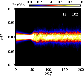
Figure 2.— Contour plot of the dust density of cm-sized pebbles averaged over the azimuthal $y$-direction, as a function of time $t$ and height over the mid-plane $z$. After the Kelvin-Helmholtz instability sets in and saturates into turbulence, the width of the dust layer stays approximately constant. The black regions contain no particles at all.

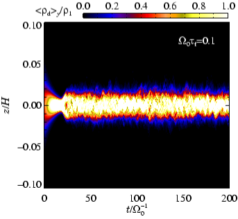
Figure 3.— Same as Fig. 2, but for dm-sized rocks with $\varOmega_{0}\tau_{\rm f}=0.1$. The sedimentation time-scale is much faster than in Fig. 2, but the width of the dust layer in the self-sustained state of turbulence is approximately the same.

Figure 4.— Dust density and Richardson number of grains with $\varOmega_{0}\tau_{\rm f}=0.02$ averaged over the azimuthal direction and over time. The dust-to-gas ratio in the mid-plane is close to unity and falls rapidly outwards. The Richardson number is approximately constant in the mid-plane and has a value around unity.

Figure 5.— Same as in Fig. 4, but for $\varOmega_{0}\tau_{\rm f}=0.1$. Although the density in the mid-plane is similar to the value for smaller grains, the dust is more settled and has less pronounced wings away from the mid-plane. The Richardson number is again around unity in the mid-plane.

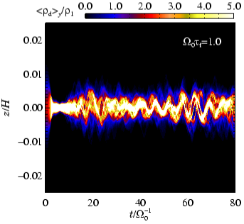
Figure 6.— Same as Fig. 3, but for m-sized boulders with $\varOmega_{0}\tau_{\rm f}=1.0$. The equilibrium scale height of the dust is around 10 times lower than for the smaller grains.

Figure 7.— Same as in Fig. 4, but for $\varOmega_{0}\tau_{\rm f}=1.0$. The Richardson number around the mid-plane is here way lower than for the smaller grains, around 0.1. This is caused by the extremely rapid settling of m-sized boulders to the mid-plane.

5. DYNAMICS AND DENSITY OF SOLIDS

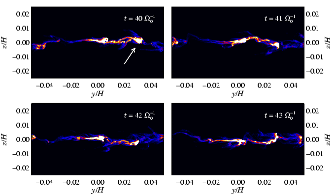
Figure 8.— Contour plot of the particle density for $\varOmega_{0}\tau_{\rm f}=1.0$. A clump, indicated by the arrow, oscillates around the mid-plane, a type of motion that is only allowed for particles with $\varOmega_{0}\tau_{\rm f}>0.5$.

In this section we focus on the dynamics and the density of the dust particles. The linear growth rate of the Kelvin-Helmholtz instability and the statistical properties of the Kelvin-Helmholtz turbulence are treated in the next two sections.

Some representative snapshots of the particle positions for run A ($\varOmega_{0}\tau_{\rm f}=0.02$, or cm-sized pebbles) are shown in Fig. 1. The particles, with an initial Gaussian density distribution, settle to the mid-plane due to gravity, on the characteristic time-scale $t_{\rm grav}=1/(\tau_{\rm f}\varOmega_{0}^{2})\approx 50$. When the width of the layer has decreased to around $0.01$ scale heights (the two middle panels of Fig. 1), some wave pattern can already be seen in the dust density. It is the most unstable $u_{z}(y)$ mode, with a wavelength that is comparable to the vertical width of the layer, that is growing in amplitude. Some shear times later, in the two bottom panels of Fig. 1, the growing mode enters the non-linear regime, and impressive patterns of breaking waves appear. The simulation then goes into a state of fully developed Kelvin-Helmholtz turbulence.

5.1. Pebbles and Rocks

In Figs. 2 and 3 we show azimuthally averaged dust density contours as a function of time for grains with friction time $\varOmega_{0}\tau_{\rm f}=0.02$ (run A) and $\varOmega_{0}\tau_{\rm f}=0.1$ (run B, decimeter-sized rocks), respectively. These two grain sizes show very similar behavior with time. In the beginning the particles move towards the mid-plane unhindered because of the lack of turbulence. The sedimentation happens much faster in run B than in run A because of the different grain sizes. When the KHI eventually sets in, the dust layer is puffed up again and quickly reaches an equilibrium configuration where the vertical distribution of dust density is practically unchanged with time.

One can already here suspect that the equilibrium dust density is indeed, as predicted analytically by S98, distributed in such a way that the flow has a constant Richardson number. In Figs. 4 and 5 we plot the time-averaged dust density and the Richardson number as a function of vertical height over the mid-plane, again for the two small grain sizes. The dust-to-gas ratio reaches unity in the mid-plane and drops down rapidly away from the mid-plane. For run A the Richardson number is approximately constant, just above unity, in the region around the mid-plane that has a significant dust density. For run B the value of the Richardson number is also constant, although somewhat smaller than for the centimeter-sized grains, because the more rapid sedimentation of these larger grains allows the disk to sustain a stronger vertical shear.

5.2. Boulders

For bodies with $\varOmega_{0}\tau_{\rm f}=1.0$ (run C, m-sized boulders), the azimuthally averaged dust density is shown in Fig. 6. These meter-sized boulders fall rapidly to the mid-plane, on a time-scale of one shear time, because they are not as coupled to the gas as smaller grains. The scale height of the boulders is very small, less than one percent of the scale height of the gas, because the grains are falling so fast that the disk can sustain a much lower Richardson number than the critical. This is also evident from Fig. 7. The Richardson number is well below unity, around $0.1$, where significant amounts of dust is present.

A major difference between the large grains and the small grains is the presence of bands in Fig. 6. The dust grains are no longer smoothly distributed over $z$, but rather appear as clumps that oscillate around the mid-plane. The oscillation of a single clump is evident from Fig. 8. Here the dust density contours are plotted at four times separated by one shear time. The clump indicated by the arrow is oscillating around the mid-plane. Such oscillatory behavior is also be expected from the following considerations. Friction ensures that small grains arrive at the mid-plane with zero residual velocity, whereas larger grains perform damped oscillations around $z=0$ with a damping time of one friction time. The distinction between the two size regimes can be derived by looking at the differential equation governing vertical settling of particles,

$$\frac{\mathrm{d}v_{z}(t)}{\mathrm{d}t}=-\varOmega_{0}^{2}z-\frac{1}{\tau_{\rm f}}v_{z}\,.$$ (25)

This second order, linear ordinary differential equation can be solved trivially (e.g. Nakagawa et al., 1986). The result is a split between two types of solutions, depending on the value of $\varOmega_{0}\tau_{\rm f}$. For $\varOmega_{0}\tau_{\rm f}\leq 0.5$ the solution is a purely exponentially decaying function. On the other hand, for $\varOmega_{0}\tau_{\rm f}>0.5$ the solutions are damped oscillations with a characteristic damping time of around one friction time. For a friction time around unity, the amplitude of the dust density in a laminar disk would still become virtually zero in just a few friction times. This is not the case in Fig. 6 where the dust scale height stays approximately constant for at least 80 friction times (the end of the simulation). The KHI is continuously pumping energy into the dust layer at the same rate as the oscillations are damped.

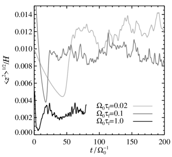
Figure 9.— The root-mean-square $z$-coordinate of the particles for the different runs. For $\varOmega_{0}\tau_{\rm f}=0.02$ and $\varOmega_{0}\tau_{\rm f}=0.1$, the width of the dust layer is around 1% of a gas scale height, whereas for meter-sized boulders with $\varOmega_{0}\tau_{\rm f}=1.0$, the strong sedimentation results in a much lower width, only around 0.25% of a scale height.

In Fig. 9 we plot the root-mean-square value of the $z$-coordinate of the particles as a function of time for all three runs. The calculated “scale height” of the cm-sized and dm-sized particles are very similar, although the larger particles have a bit lower scale height than the smaller particles. The m-sized particles have a scale height of about one quarter of a percent of that of the gas.

5.3. Maximum Density and Clumping

It is of great relevance for planetesimal formation to find the highest dust density that is permitted in the saturated Kelvin-Helmholz turbulence. Both coagulation and gravitational fragmentation depend strongly on the mass density of the dust layer. High densities can occur not only when the gas flow or the size of the boulders allow for a high mid-plane density, but also in certain points of the turbulent flow where dust particles tend to accumulate. The latter can only be explored in computer simulations, so we examine the maximum dust density in any grid point in more detail in this section.

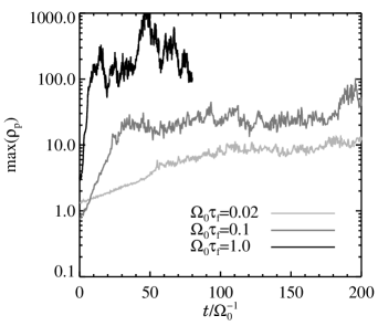
Figure 10.— The maximum dust density in any grid cell as a function of time, in units of the gas mid-plane density, as a function of time. The value is much higher than the azimuthally averaged mid-plane densities (presented in previous figures).

The maximum mass density of dust particles in any grid cell is plotted in Fig. 10 as a function of time. Even though the mid-plane dust-to-gas ratio is on the average of the order unity for all grain sizes, the maximum density is much higher at all times, especially for meter-sized particles where the maximum dust-to-gas ratio can be up to one thousand. Decimeter-sized particles have a maximum dust-to-gas ratio of around 20 at all times, whereas the value for centimeter-sized particles is around 10. This is potentially important for building planetesimals. Even if the critical density for gravity-aided planetesimal formation is not reached globally, this is still possible in certain regions of the turbulent flow. Such a gravoturbulent formation of planetesimals was proposed by Johansen et al. (2006) to lead to the formation of planetesimals in a magnetorotationally turbulent gas.

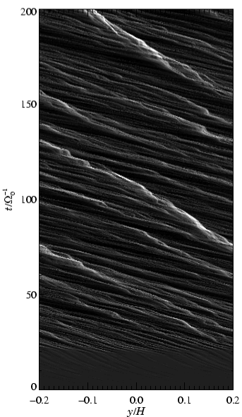
Figure 11.— Vertically averaged dust density of rocks with $\varOmega_{0}\tau_{\rm f}=0.1$ as a function of azimuthal coordinate $y$ and time $t$. The clumping mechanism is evident from the plot. Regions of high dust-to-gas ratio (light) move slower than regions of low dust-to-gas ratio (gray), seen in the different slopes of the bright and dark wisps on the plot, causing the high density clumps to be continuously fed by low density material. One also sees the rarefaction tail going to the left of the dense clumps and the shock front that is formed against the sub-Keplerian stream.

In Fig. 11 we plot contours of the vertically averaged dust density as a function of azimuthal coordinate $y$ and time $t$ for decimeter-sized rocks (run B). It is evident that the dust density has a strong non-axisymmetric component once the Kelvin-Helmholtz turbulence is fully developed. Dense clumps are seen as white stripes, while regions of lower dust-to-gas ratio are gray. A simple way to quantify the amount of non-axisymmetry is to look at the mean deviation of the dust density from the average density. We define the azimuthal clumping factor $c_{y}$ as

$$c_{y}=\frac{\sqrt{\langle[n_{y}(y)-\langle n_{y}(y)\rangle]^{2}\rangle}}{\langle n_{y}(y)\rangle}\,.$$ (26)

Here $n_{y}(y)\equiv\langle n(y,z)\rangle_{z}$ is the dust number density averaged over the vertical direction. Axisymmetry implies $c_{y}=0$, whereas higher values of $c_{y}$ imply stronger and stronger non-axisymmetry. We plot in Fig. 12 the azimuthal clumping factor as a function of time for all three values of the friction time. For centimeter and decimeter particles the clumping is of the order unity, or in other words, the average grid point has a density variation from the average that is on the same order as the average, i.e. very strong clumping. For meter-sized particles the azimuthal clumping is even stronger.

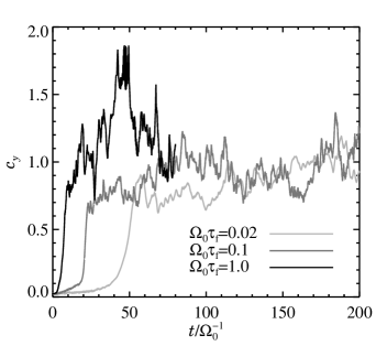
Figure 12.— Azimuthal clumping factor $c_{y}$ versus time for all three grain sizes. A value of around unity corresponds to strong clumping with the average point being $100\%$ away in density from the average density.

The tendency for the dust particles to clump is a consequence of the sub-Keplerian velocity of the gas. Turning again to Fig. 11, one sees that brighter regions move at a lower speed (relative to the Keplerian speed) than dark regions do. The speed of a clump is evident from the absolute value of the angle between the tilted time-space wisp and the time-axis. Bright wisps have a higher angle with the time-axis than dark wisps. This instability is very related to the streaming instability found by Youdin & Goodman (2005), although in our simulations the clumping happens in the $(y,z)$-plane and not the $(x,z)$-plane as in the analysis by Youdin & Goodman. Still the instability is powered in both planes by the dependence of the dust velocity on the dust-to-gas ratio, so we consider the instability in the $(y,z)$-plane a special case of the streaming instability. We refer to Youdin & Goodman (2005) for a linear stability analysis of the coupled gas and dust flow. In the rest of this section we instead focus on describing the non-linear outcome of the streaming instability with a simple analogy to a hydrodynamical shock.

Using the derivations given by Nakagawa et al. (1986) for the equilibrium gas and dust velocities as a function of the dust-to-gas mass ratio $\epsilon$, one can write up the azimuthal velocity component of the dust as

$$w_{y}=\frac{1+\epsilon}{(1+\epsilon)^{2}+(\varOmega_{0}\tau_{\rm f})^{2}}u_{y}^{(0)}\,.$$ (27)

Thus clumps with a high dust-to-gas ratio move slower, relative to the Keplerian speed, than clumps with a low dust-to-gas ratio. The small clumps crash into the big clumps and form larger structures. At the same time, the large clumps steepen up against the direction of the sub-Keplerian flow and develop an escaping tail downstream. This is qualitatively similar to a shock. Considering the continuity equation of the dust-to-gas ratio

$$\frac{\partial\epsilon}{\partial t}=-w_{y}\frac{\partial\epsilon}{\partial y}-\epsilon\frac{\partial w_{y}}{\partial y}\,,$$ (28)

and inserting equation (27) in the limit of small Stokes numbers $\varOmega_{0}\tau_{\rm f}\ll 1$, equation (28) can be reduced to

$$\frac{\partial\epsilon}{\partial t}=-\frac{u_{y}^{(0)}}{(1+\epsilon)^{2}}\frac{\partial\epsilon}{\partial y}\,,$$ (29)

qualitatively similar to the advection equation of fluid dynamics. The shock behavior of the clumps arises because the advection velocity $u_{y}^{(0)}/(1+\epsilon)^{2}$ depends on the dust-to-gas ratio.

5.4. Varying the Global Dust-to-gas Ratio

It is of great interest to investigate the dependence of the mid-plane dust density on the global dust-to-gas ratio in the saturated state of Kelvin-Helmholtz turbulence. Increasing the dust-to-gas ratio beyond the interstellar value should potentially lead to the creation of a very dense mid-plane of dust that the gas is not able to lift up, making the dust layer dense enough to undergo gravitational fragmentation (Sekiya, 1998; Youdin & Shu, 2002; Youdin & Chiang, 2004).

The analytically predicted mid-plane dust-to-gas ratio $\epsilon_{1}$ is found by applying the normalization

$$\int_{-\infty}^{\infty}\rho_{1}\epsilon(z)\mathrm{d}z=\varSigma_{\rm d}$$ (30)

to the constant Richardson number dust density of equation (20). Here $\varSigma_{\rm d}$ is the dust column density, a free parameter that we set through the global dust-to-gas ratio $\epsilon_{0}$ as $\varSigma_{\rm d}=\epsilon_{0}\varSigma$. We have approximated the gas density by the gas density in the mid-plane $\rho_{1}$, because for $z\ll H$, the variation in gas density is insignificant compared to the variation in dust density. We proceed by inserting the expression for the dust density in a disk with a constant Richardson number, from equation (20), into the integral in equation (30). Defining the parameter

$$\chi=\frac{\sqrt{\epsilon_{1}(2+\epsilon_{1})}}{1+\epsilon_{1}}\,,$$ (31)

the integration yields

$$-2\chi+\ln\left(\frac{1+\chi}{1-\chi}\right)=\frac{\varSigma_{\rm d}}{H_{\rm d}\rho_{1}}\,.$$ (32)

This is a transcendental equation that we solve numerically for $\chi$ as a function of the input parameters $H_{\rm d}$, given by equation (21), and $\varSigma_{\rm d}$. Once $\chi$ is calculated, then the dust-to-gas ratio in the mid-plane $\epsilon_{1}$ is known from equation (31).

Figure 13.— Mid-plane dust-to-gas ratio $\epsilon_{1}$ as a function of global dust-to-gas ratio $\epsilon_{0}$. The dotted line shows the analytical value for a dust density with a constant Richardson number of ${\rm Ri}_{\rm c}=1.0$, while the stars show the result of the numerical simulations for different values of the global dust-to-gas ratio. The results agree nicely, giving support to the idea that a dust-to-gas ratio that is higher than the interstellar value can give rise to high enough mid-plane dust density for a gravitational instability in the dust layer.

In Fig. 13 we plot the analytical mid-plane dust-to-gas ratio $\epsilon_{1}$ as a function of the global dust-to-gas ratio $\epsilon_{0}$ (dotted line). The non-linear behavior of $\epsilon_{1}$ is evident, and already for $\epsilon_{0}=0.1$ does the mid-plane dust-to-gas ratio approach $\epsilon_{1}=100$, which should be enough to have a gravitational instability in the dust layer. We also run numerical simulations with an increased global dust-to-gas ratio (runs Be2, Be5 and Be10, see Table 1) to see if a mid-plane dust density cusp develops as predicted. The resulting mid-plane dust-to-gas ratio is indicated with stars in Fig. 13. To avoid having a very low time-step, because of the strong friction that the dust exerts on the gas when the global dust-to-gas ratio is increased, we have locally increased the friction time in regions of very high dust-to-gas ratio. This approach conserves total momentum because the friction force on the gas and on the dust are made lower at the same time. In the regions where the friction time is increased, the dust-to-gas ratio is so high that gas is dragged along with the particles anyway, so the precise value of the friction time does not matter. As seen in Fig. 13 the mid-plane dust-to-gas ratio does indeed increase non-linearly with global dust-to-gas ratio, following a curve that is within a factor of two of the analytical curve. This gives support to the theory that an increased global dust-to-gas ratio, e.g. due to solids that are transported from the outer part of the disk into the inner part, can lead to such a high dust-to-gas ratio in the disk mid-plane that the dust layer fragments to form planetesimals (Youdin & Shu, 2002).

6. GROWTH RATES

The simulations presented so far all imply a critical Richardson number that is of the order unity, rather than the classically adopted value of $1/4$. This confirms the findings of GO05 that shear flows with a Richardson number that is higher than the classical value are actually unstable when the Coriolis force is included in the calculations. To quantify the linear growth of the instability we have run simulations of initial conditions with a constant Richardson number and measured the growth rates of the KHI. Because we are only interested in the linear regime, we have chosen for simplicity to treat dust as a fluid rather than as particles. Thus we solve equations similar to equations (13)–(15) for the dust velocity field ${\boldsymbol{w}}$ including an advection term $({\boldsymbol{w}}\cdot{\boldsymbol{\nabla}}){\boldsymbol{w}}$. A continuity equation similar to equation (9) for the logarithmic dust number density $\ln n$ is solved at the same time.

We consider initial conditions with a constant Richardson number, in the range between $0.1$ and $2.0$, as given by equation (20). The dust-to-gas ratio in the mid-plane $\epsilon_{1}$ is known from equations (31) and (32). To avoid any effects of dust settling, we set the friction time to $\varOmega_{0}\tau_{\rm f}=0.001$. The gravitational settling time is then as high as $1000\varOmega_{0}^{-1}$, and since this is much longer than the duration of the linear growth, the effect on the measured growth rate is insignificant. The vertical velocity of the dust is set to the terminal settling velocity $w_{z}=-\tau_{\rm f}\varOmega_{0}^{2}z$. Since the dust velocity is not zero, the gas will feel some friction from the falling dust. The vertical component of the equation of motion of the gas is

$$\frac{\partial u_{z}}{\partial t}=-\varOmega_{0}^{2}z-\frac{1}{\gamma}c_{\rm s}^{2}\frac{\partial\ln\rho}{\partial z}-\frac{\epsilon}{\tau_{\rm f}}(u_{z}-w_{z})\,.$$ (33)

We insert the terminal velocity expression for the dust velocity into equation (33) and look for equilibrium solutions with $u_{z}=\partial u_{z}/\partial t=0$. The equation is then reduced to

$$0=-(1+\epsilon)\varOmega_{0}^{2}z-\frac{1}{\gamma}c_{\rm s}^{2}\frac{\partial\ln\rho}{\partial z}\,.$$ (34)

The drag force exerted by the falling dust on the gas mimics a vertical gravity, and therefore we have combined it with the regular gravity term. In a way it is the gravity on the dust that the gas feels, only it is transferred to the gas component through the drag force. One can interpret this as the gas feeling a stronger gravity $\varOmega_{0}^{\prime}=\sqrt{1+\epsilon}\varOmega_{0}$ in places of high dust-to-gas ratio, which leads to the creation of a small cusp in the gas density around the mid-plane. Inserting now equation (20) into equation (34) and applying the boundary condition $\rho(z=0)=\rho_{1}$ yields

$$\ln\rho(z)=\left\{\begin{array}[]{l}\ln\rho_{1}+\frac{\gamma\varOmega_{0}^{2}H_{\rm d}^{2}}{c_{\rm s}^{2}}\left[\frac{1}{1+\epsilon_{1}}-\sqrt{\frac{z^{2}}{H_{\rm d}^{2}}+\frac{1}{(1+\epsilon_{1})^{2}}}\right]\\ \hskip 113.81102pt{\rm for}\,\,|z|<z_{\rm d}\\ \ln\rho_{1}+\frac{\gamma\varOmega_{0}^{2}H_{\rm d}^{2}}{c_{\rm s}^{2}}\left[-\frac{1}{2}\frac{z^{2}}{H_{\rm d}^{2}}-\frac{\epsilon_{1}^{2}}{2(1+\epsilon_{1})^{2}}\right]\\ \hskip 113.81102pt{\rm for}\,\,|z|\geq z_{\rm d}\end{array}\right.\,.$$ (35)

The cusp around the mid-plane, caused by the extra gravity imposed by the falling dust on the gas, is shown in Fig. 14. The variation in density from a normal isothermal disk is only a few parts in ten thousand, so the effect is not big. On the other hand, it is important to have a complete equilibrium solution as the initial condition for the measurement of the linear growth of the instability, as otherwise dynamical effects could dominate over the growth.

We measure the linear growth rate of the KHI by prescribing a dust-to-gas ratio according to equation (20) and a gas density according to equation (35). We then set the velocity fields of gas and dust according to the expressions derived in Nakagawa et al. (1986). The width of a dust layer with a constant Ri depends on the value of Ri according to equation (21), so we have made sure to always resolve the unstable wavelengths by making the box larger with increasing Ri. The fluid simulations are all done with a grid resolution of $N_{y}\times N_{z}=256\times 128$.

The measured growth rates are shown in Fig. 15. At a Richardson number close to zero, the growth rate is similar in magnitude to the rotation frequency $\varOmega_{0}$ of the disk, whereas for larger values of the Richardson number, the growth rate falls rapidly. We find that there is growth out to at least ${\rm Ri}=2.0$, with a growth rate approaching $\omega=0.01\varOmega_{0}$. There is no evidence for a cut-off in the growth rate at the classical value of the critical Richardson number of $0.25$. The range of unstable Richardson numbers is in good agreement with the mid-plane Richardson number in the particle simulations shown in Figs. 4 and 5. This is another confirmation that the critical Richardson number is around unity or higher when the Coriolis force is included in the calculations. On the other hand, when the Keplerian shear is included, growth rates higher than the shear rate $3/2\varOmega_{0}$ are expected to be required to overcome the shear (Ishitsu & Sekiya, 2003), although numerical simulations in 3-D would be required to address these analytical results in detail.

Figure 14.— The logarithmic gas density as a function of height over the mid-plane $z$ in the presence of falling dust. The drag force exerted on the gas by the falling dust mimics an extra gravity near the mid-plane, making the gas scale height slightly lower close to the mid-plane. The result is the formation of a cusp, although of a very moderate amplitude of about 1/10000 compared to a disk with no dust sedimentation (dotted line).

Our measured growth rates are somewhat smaller than in GO05, but we believe that this is due to the different Coriolis force term in the present work. Changing the factor $-1/2$ to a factor $-2$ in equations (2) and (14) yields very similar growth rates to GO05. The factor $-1/2$ is a consequence of the advection of the Keplerian rotation velocity when fluid parcels move radially, an effect that was not included in the simulations of GO05.

Figure 15.— Initial growth rate of the Kelvin-Helmholtz instability as a function of the Richardson number ${\rm Ri}$. There is measurable growth out to at least ${\rm Ri}=2.0$, which is way beyond the classical value of the critical Richardson number of ${\rm Ri}_{\rm c}=0.25$.

7. PROPERTIES OF KELVIN-HELMHOLTZ TURBULENCE

7.1. Diffusion Coefficient

The effect of turbulence on the vertical distribution of dust grains can be quantified as a diffusion process with the turbulent diffusion coefficient $D_{\rm t}$ (Cuzzi et al., 1993; Dubrulle et al., 1995; Schräpler & Henning, 2004). Assuming that $D_{\rm t}$ is a constant, i.e. independent of the height over the mid-plane, the equilibrium between vertical settling of dust with velocity $w_{z}=-\tau_{\rm f}\varOmega_{0}^{2}z$ and turbulent diffusion implies a vertical distribution of the dust-to-gas ratio $\epsilon(z)$ that is Gaussian around the mid-plane (Dubrulle et al., 1995),

$$\epsilon=\epsilon_{1}\exp[-z^{2}/(2H_{\epsilon}^{2})]\,,$$ (36)

with the dust-to-gas ratio scale height given by the expression $H_{\epsilon}^{2}=D_{\rm t}/(\tau_{\rm f}\varOmega_{0}^{2})$. Writing now $D_{\rm t}=\delta_{\rm t}H^{2}\varOmega_{0}$, we get

$$\delta_{\rm t}=\left(\frac{H_{\epsilon}}{H}\right)^{2}\varOmega_{0}\tau_{\rm f}\,.$$ (37)

Using equation (37), one can translate the scale-height of the dust-to-gas ratio $H_{\epsilon}$ into a turbulent diffusion coefficient $\delta_{\rm t}$. Such an approach has been used to calculate the turbulent diffusion coefficient of magnetorotational turbulence (Johansen & Klahr, 2005). An obvious difference between Kelvin-Helmholtz turbulence and magnetorotational turbulence is that dust itself plays the active role for the first, whereas for the latter the presence of dust does not change the turbulence in any way, because the local dust-to-gas ratio is assumed to be low. Thus, for Kelvin-Helmholtz turbulence we expect the diffusion coefficient to depend on the friction time $\delta_{\rm t}=\delta_{\rm t}(\tau_{\rm f})$.

The calculated turbulent diffusion coefficients for all the simulations are shown in Table 2. For the dust-to-gas ratio scale height we have, for simplicity, used the root-mean-square of the $z$-coordinates of all the particles. The measured coefficients are extremely low, on the order of $10^{-6}$. If we assume that the turbulent viscosity $\alpha_{\rm t}$ is similar to the turbulent diffusion coefficient $\delta_{\rm t}$, then one sees that Kelvin-Helmholtz turbulence is much weaker than magnetorotational turbulence where $\alpha$-values from $10^{-3}$ to unity are found. There is a good agreement between the diffusion coefficients of run B and run Br512 (which has twice the grid and particle resolution). This shows that the solution has converged and that $256\times 128$ is indeed a sufficient resolution to say something meaningful about the Kelvin-Helmholtz turbulence. For the simulations with an increased global dust-to-gas ratio (runs Be2, Be5 and Be10), the dust scale height falls with increasing dust-to-gas ratio. This is to be expected from equation (20), because of the cusp of high dust density that forms around the mid-plane when $\epsilon_{1}\gg 1$. The diffusion coefficient for $\varOmega_{0}\tau_{\rm f}=1.0$ is around $50\%$ lower than for $\varOmega_{0}\tau_{\rm f}=0.1$. Here the strong vertical settling of the dust has decreased the width of the dust layer significantly, and thus the diffusion coefficient is also much lower.

Turbulent transport coefficients such as $\alpha_{\rm t}$ and $\delta_{\rm t}$ have an inherent dependence on the width of the turbulent region. Thus the “strength” of the turbulence is better illustrated by the actual turbulent velocity fluctuations. In Fig. 16 we plot the root-mean-square of the vertical gas velocity as a function of height over the mid-plane. In the mid-plane, the value is quite independent of the friction time, whereas the width of the turbulent region is much smaller for $\varOmega_{0}\tau_{\rm f}=1$. Thus the turbulence in itself is not weaker, only the turbulent region is smaller, and that means that the transport coefficients are accordingly small.

7.2. Comparison With Analytical Work

It is evident from Table 2 that the diffusion coefficient depends on the friction time. In the limit of small Stokes numbers, the constant Richardson number density distribution formulated by S98 predicts that the vertical dust density distribution should not depend on friction time, and thus, according to equation (37), that the diffusion coefficient should be proportional to the friction time. The ratio of the diffusion coefficient of run B to that of run A is $8.9/3.0\approx 3$, and not $0.1/0.02=5$ as would give rise to the same scale height. The factor two difference can be (trivially) attributed to the slight difference in scale heights for the two runs. The squared value is different by almost a factor of two, an indication that vertical settling is not completely negligible for $\varOmega_{0}\tau_{\rm f}=0.1$.

Table 2Diffusion Coefficients

Run	$\varOmega_{0}\tau_{\rm f}$	$\sqrt{\langle z^{2}\rangle}/H$	$\delta_{\rm t}/10^{-6}$
A	$0.02$	$0.0121\pm 0.0010$	$3.0\pm 0.5$
B	$0.10$	$0.0094\pm 0.0008$	$8.9\pm 1.5$
C	$1.00$	$0.0025\pm 0.0004$	$6.5\pm 2.4$
Be2	$0.10$	$0.0081\pm 0.0006$	$6.5\pm 1.0$
Be5	$0.10$	$0.0047\pm 0.0003$	$2.2\pm 0.3$
Be10	$0.10$	$0.0031\pm 0.0002$	$1.0\pm 0.1$
Br512	$0.10$	$0.0086\pm 0.0005$	$7.5\pm 0.8$

Note. — Col. (1): Name of run. Col. (2): Stokes number. Col. (3): Dust scale height. Col. (4): Diffusion coefficient derived from equation (37).

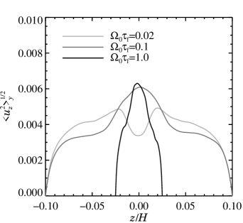
Figure 16.— Root-mean-square of the vertical gas velocity as a function of height over the mid-plane. The value is quite independent of Stokes number, but the width of the turbulent region is very small for $\varOmega_{0}\tau_{\rm f}=1$ because of the strong vertical settling of m-sized boulders. The boundary conditions set the vertical speed to zero at the boundaries.

The strength of the Kelvin-Helmholtz turbulence has also been estimated analytically by Cuzzi et al. (1993). They find that the turbulent viscosity $\nu_{\rm t}$ should be approximately (their equation [21])

$$\nu_{\rm t}\approx\frac{(\eta v_{\rm K})^{2}}{\varOmega_{0}{\rm Re}^{*2}}\,,$$ (38)

where $v_{\rm K}$ is the Keplerian velocity, $\eta$ is the pressure gradient parameter defined in equation (6) and ${\rm Re^{*}}$ is the critical Reynolds number at which the flow becomes unstable. This value can be approximated by the Rossby number ${\rm Ro}$, the ratio between the advection and Coriolis force terms of the flow. Dobrovolskis et al. (1999) estimate a value of ${\rm Ro}\approx 20\ldots 30$. Using the approximation $\eta\approx c_{\rm s}^{2}/v_{\rm K}^{2}$, equation (38) can be written as

$$\nu_{\rm t}=D_{\rm t}=\frac{\eta}{{\rm Ro}^{2}}c_{\rm s}^{2}\varOmega_{0}^{-1}\,,$$ (39)

which appears in its dimensionless form simply as

$$\delta_{\rm t}=\frac{\eta}{{\rm Ro}^{2}}\,.$$ (40)

With $\beta=-0.1$, equation (8) gives $\eta=0.003$. Using ${\rm Ro}=20\ldots 30$, equation (40) gives $\delta_{\rm t}\sim 3\ldots 8\times 10^{-6}$, quite comparable to the values in Table 2. On the other hand, equation (38) does not produce a dust density distribution with a constant Richardson number, and would thus greatly overestimate the diffusion coefficient for even smaller grains. This is also noted by Cuzzi & Weidenschilling (2005) who constrain the validity of equation (38) to $\varOmega_{0}\tau_{\rm f}>0.01$. Thus our measured diffusion coefficients are actually in good agreement with both Cuzzi et al. (1993) and with S98.

8. CONCLUSIONS

The onset of the Kelvin-Helmholtz instability in protoplanetary disks has been known for decades to be the main obstacle for the formation of planetesimals via a gravitational collapse of the particle subdisk. Thus the study of the Kelvin-Helmholtz instability is one of the most intriguing problems of planetesimal formation. It is also a challenging problem to solve, both analytically and numerically, because of the coevolution of the two components gas and dust. Whereas turbulence normally arises from the gas flow alone, in Kelvin-Helmholtz turbulence the dust grains take the active part as the source of turbulence by piling up around the mid-plane and thus turning the energetically favored vertical rotation profile into an unstable shear. Planetesimal formation would be deceptively simple could the solids only sediment unhindered, but nature’s dislike of thin shear flows precludes this by making the mid-plane turbulent.

In the current work we have shown numerically that when the dust particles are free to move relative to the gas, the Kelvin-Helmholtz turbulence acquires an equilibrium state where the vertical settling of the solids is balanced by the turbulent diffusion away from the mid-plane. For cm-sized pebbles and dm-sized rocks, we find that the dust component forms a layer that has a constant Richardson number. We thus confirm the analytical predictions by Sekiya (1998) for the first time in numerical simulations.

In the saturated turbulence we find the formation of highly overdense regions of solids, not in the mid-plane, but embedded in the turbulent flow. The clumping is very related to the streaming instability found by Youdin & Goodman (2005). Dust clumps with a density that is equal to or higher than the gas density orbit at the Keplerian velocity, so the clumps overtake sub-Keplerian regions of lower dust density. Thus the dense clumps continue to grow in size and in mass. The final size of a dust clump is given by a balance between this feeding and the loss of material in a rarefaction tail that is formed behind the clump along the sub-Keplerian stream. The gravitational fragmentation of the single clumps into planetesimals is more likely than the whole dust layer fragmenting, because the local dust density in the clumps can be more than an order of magnitude higher than the azimuthally averaged mid-plane density. This process is very much related to the gravoturbulent formation of planetesimals in turbulent magnetohydrodynamical flows (Johansen, Klahr, & Henning, 2006).

A full understanding of the role of Kelvin-Helmholtz turbulence in protoplanetary disks must eventually rely on simulations that include the effect of the Keplerian shear, so future simulations have to be extended into three dimensions. One can to first order expect that growth rates of the KHI larger than the shear rate $\varOmega_{0}$ are required for a mode to grow in amplitude faster than it is being sheared out (Ishitsu & Sekiya, 2003), but so far it is an open question in how far the radial shear changes the appearance of the self-sustained state of Kelvin-Helmholz turbulence. Including furthermore the self-gravity between the dust particles, it will become feasible to study the formation of planetesimals in one self-consistent computer simulation and possibly to answer one of the outstanding questions in the planet formation process.

References

- Armitage (1998) Armitage, P. J. 1998, ApJ, 501, L189+
- Balbus & Hawley (1991) Balbus, S. A., & Hawley, J. F. 1991, ApJ, 376, 214
- Balbus et al. (1996) Balbus, S. A., Hawley, J. F., & Stone, J. M. 1996, ApJ, 467, 76
- Barge & Sommeria (1995) Barge, P., & Sommeria, J. 1995, A&A, 295, L1
- Blum & Wurm (2000) Blum, J., & Wurm, G. 2000, Icarus, 143, 138
- Brandenburg et al. (1995) Brandenburg, A., Nordlund, Å., Stein, R.F., & Torkelsson, U. 1995, ApJ, 446, 741
- Brandenburg & Sarson (2002) Brandenburg, A., & Sarson, G. R. 2002, Physical Review Letters, 88, 055003
- Brandenburg (2003) Brandenburg, A. 2003, in Advances in nonlinear dynamos (The Fluid Mechanics of Astrophysics and Geophysics, Vol. 9), ed. A. Ferriz-Mas & M. Núñez (Taylor & Francis, London and New York), 269-344
- Chandrasekhar (1961) Chandrasekhar, S. 1961, Hydrodynamic and hydromagnetic stability
- Chavanis (2000) Chavanis, P. H. 2000, A&A, 356, 1089
- Cuzzi et al. (1993) Cuzzi, J. N., Dobrovolskis, A. R., & Champney, J. M. 1993, Icarus, 106, 102
- Cuzzi & Weidenschilling (2005) Cuzzi, J. N. & Weidenschilling, S. J. 2005, in Meteorites in the Early Solar System - II, University of Arizona Press and the Lunar and Planetary Institute
- Dobler et al. (2006) Dobler, W., Stix, M., & Brandenburg, A. 2006, ApJ, in press
- Dobrovolskis et al. (1999) Dobrovolskis, A. R., Dacles-Mariani, J. S., & Cuzzi, J. N. 1999, J. Geophys. Res., 104, 30805
- Dubrulle et al. (1995) Dubrulle, B., Morfill, G., & Sterzik, M. 1995, Icarus, 114, 237
- Dullemond & Dominik (2005) Dullemond, C. P., & Dominik, C. 2005, A&A, 434, 971
- Fleming & Stone (2003) Fleming, T., & Stone, J. M. 2003, ApJ, 585, 908
- Fromang et al. (2002) Fromang, S., Terquem, C., & Balbus, S. A. 2002, MNRAS, 329, 18
- Fromang & Nelson (2005) Fromang, S., & Nelson, R. P. 2005, MNRAS, 364, L81
- Gammie (1996) Gammie, C. F. 1996, ApJ, 457, 355
- Goldreich & Ward (1973) Goldreich, P., & Ward, W. R. 1973, ApJ, 183, 1051
- Gómez & Ostriker (2005) Gómez, G. C., & Ostriker, E. C. 2005, ApJ, 630, 1093
- Haugen & Brandenburg (2004) Haugen, N. E., & Brandenburg, A. 2004, Phys. Rev. E, 70, 026405
- Hawley et al. (1995) Hawley, J. F., Gammie, C. F., & Balbus, S. A. 1995, ApJ, 440, 742
- Henning et al. (2006) Henning, Th., Dullemond, C.P., Dominik, C., & Wolf, S. (2006), to appear in Planet Formation: Observations, Experiments and Theory, ed. H. Klahr and W. Brandner (Cambridge University Press, Cambridge).
- Hodgson & Brandenburg (1998) Hodgson, L. S., & Brandenburg, A. 1998, A&A, 330, 1169
- Ishitsu & Sekiya (2002) Ishitsu, N., & Sekiya, M. 2002, Earth, Planets, and Space, 54, 917
- Ishitsu & Sekiya (2003) Ishitsu, N., & Sekiya, M. 2003, Icarus, 165, 181
- Johansen et al. (2004) Johansen, A., Andersen, A. C., & Brandenburg, A. 2004, A&A, 417, 361
- Johansen & Klahr (2005) Johansen, A., & Klahr, H. 2005, ApJ, 634, 1353
- Johansen et al. (2006) Johansen, A., Klahr, H., & Henning, Th. 2006, ApJ, 636, 1121
- Keppens & Tóth (1999) Keppens, R., & Tóth, G. 1999, Physics of Plasmas, 6, 1461
- Keppens et al. (1999) Keppens, R., Tóth, G., Westermann, R. H. J., & Goedbloed, J. P. 1999, Journal of Plasma Physics, 61, 1
- Klahr & Henning (1997) Klahr, H. H., & Henning, T. 1997, Icarus, 128, 213
- Klahr & Bodenheimer (2003) Klahr, H. H., & Bodenheimer, P. 2003, ApJ, 582, 869
- Klahr & Bodenheimer (2006) Klahr, H. H., & Bodenheimer, P. 2006, ApJ, in press
- Li et al. (2001) Li, H., Colgate, S. A., Wendroff, B., & Liska, R. 2001, ApJ, 551, 874
- Nakagawa et al. (1986) Nakagawa, Y., Sekiya, M., & Hayashi, C. 1986, Icarus, 67, 375
- Safronov (1969) Safronov, V. S. 1969, Evoliutsiia doplanetnogo oblaka. (English transl.: Evolution of the Protoplanetary Cloud and Formation of Earth and the Planets, NASA Tech. Transl. F-677, Jerusalem: Israel Sci. Transl. 1972)
- Schräpler & Henning (2004) Schräpler, R. & Henning, T. 2004, ApJ
- Sekiya (1998) Sekiya, M. 1998, Icarus, 133, 298
- Sekiya & Ishitsu (2000) Sekiya, M., & Ishitsu, N. 2000, Earth, Planets, and Space, 52, 517
- Semenov et al. (2004) Semenov, D., Wiebe, D., & Henning, T. 2004, A&A, 417, 93
- Varniere & Tagger (2005) Varniere, P., & Tagger, M. 2005, A&A in press, astro-ph/0511684
- Weidenschilling (1977) Weidenschilling, S. J. 1977, MNRAS, 180, 57
- Weidenschilling (1980) Weidenschilling, S. J. 1980, Icarus, 44, 172
- Weidenschilling & Cuzzi (1993) Weidenschilling, S. J., & Cuzzi, J. N. 1993, in Protostars and Planets III, 1031–1060
- Wünsch et al. (2005) Wünsch, R., Klahr, H., & Różyczka, M. 2005, MNRAS, 362, 361
- Youdin & Shu (2002) Youdin, A. N., & Shu, F. H. 2002, ApJ, 580, 494
- Youdin & Chiang (2004) Youdin, A. N., & Chiang, E. I. 2004, ApJ, 601, 1109
- Youdin & Goodman (2005) Youdin, A. N., & Goodman, J. 2005, ApJ, 620, 459
- Youdin (2005a) Youdin, A. N. 2005, astro-ph/0508659
- Youdin (2005b) Youdin, A. N. 2005, astro-ph/0508662