On the properties of fractal cloud complexes

Abstract

We study the physical properties derived from interstellar cloud complexes having a fractal structure. We first generate fractal clouds with a given fractal dimension and associate each clump with a maximum in the resulting density field. Then, we discuss the effect that different criteria for clump selection has on the derived global properties. We calculate the masses, sizes and average densities of the clumps as a function of the fractal dimension ($D_{f}$) and the fraction of the total mass in the form of clumps ($\epsilon$). In general, clump mass does not fulfill a simple power law with size of the type $M_{cl}\varpropto R_{cl}^{\gamma}$, instead the power changes, from $\gamma\simeq 3$ at small sizes to $\gamma<3$ at larger sizes. The number of clumps per logarithmic mass interval can be fitted to a power law $N_{cl}\varpropto M_{cl}^{-\alpha_{M}}$ in the range of relatively large masses, and the corresponding size distribution is $N_{cl}\varpropto R_{cl}^{-\alpha_{R}}$ at large sizes. When all the mass is forming clumps ($\epsilon=1$) we obtain that as $D_{f}$ increases from $2$ to $3$ $\alpha_{M}$ increases from $\sim 0.3$ to $\sim 0.6$ and $\alpha_{R}$ increases from $\sim 1.0$ to $\sim 2.1$. Comparison with observations suggests that $D_{f}\simeq 2.6$ is roughly consistent with the average properties of the ISM. On the other hand, as the fraction of mass in clumps decreases ($\epsilon<1$) $\alpha_{M}$ increases and $\alpha_{R}$ decreases. When only $\sim 10\%$ of the complex mass is in the form of dense clumps we obtain $\alpha_{M}\simeq 1.2$ for $D_{f}=2.6$ (not very different from the Salpeter value $1.35$), suggesting this a likely link between the stellar initial mass function and the internal structure of molecular cloud complexes.

1 Introduction

The fact that the interstellar medium (ISM) has a hierarchical and self-similar structure when observed with sufficiently high dynamic range, is interpreted as evidence of an underlying fractal structure (Scalo, 1990). The boundaries of the projected images of interstellar clouds are irregular curves whose fractal dimension is around $\sim 1.3$ (e.g. Falgarone et al., 1991; Lee, 2004). Apparently this is a universal result which does not depend on whether tracers of atomic, molecular or dust components are used, whether clouds are selfgravitating or not, etc (Williams et al., 2000). The fractal dimension of the projected boundaries is usually associated with a three-dimensional fractal dimension $D_{f}\simeq 2.3$ for the ISM (e.g. Beech, 1992). It has been argued that a fractal ISM with $D_{f}\simeq 2.3$ could account for the observed mass and size distributions of the interstellar clouds (Elmegreen & Falgarone, 1996), as well as for the intercloud medium properties (Elmegreen, 1997a), and even for the stellar initial mass function (Elmegreen, 1997b, 1999).

In a previous paper (Sánchez et al., 2005) we studied the effect that the projection of clouds has on the estimation of the fractal dimension, and we concluded that a value around $\sim 1.3$ for the projected boundaries is more consistent with three-dimensional clouds having $D_{f}\sim 2.6\pm 0.1$. The application of $\Delta$-variance techniques to Polaris Flare cloud by Stutzki et al. (1998) yielded a fractal dimension for the cloud surfaces $\simeq 2.6$ (see also Bensch et al., 2001). Elmegreen (2002) simulated fractal brownian motion clouds with average fractal dimension $\sim 2.75$ and obtained properties in gross agreement with observations. A fractal medium with a relatively high $D_{f}$ value can reproduce observations of HII regions surrounding stars (Wood et al., 2005). Henriksen (1986, 1991) used a gravitationally driven turbulence model to study the properties of giant molecular clouds suggesting that a dimension $\simeq 2.7$ could be necessary to explain the observed properties. Also Fleck (1996) analyzed the properties of the turbulent, non-self-gravitating, neutral component of the ISM by using a model of compressible turbulence, concluding that the compression parameter that better reproduces observations is such that $D_{f}\simeq 2.5$.

It is important to quantify the degree of complexity (through, for example, the fractal dimension) as a first step towards understanding the physical mechanisms responsible for structuring the ISM. In models of fractally homogeneous turbulence the fractal dimension of fully developed turbulence is $2.5<D_{f}<2.75$ (Hentschel & Procaccia, 1982). On the other hand, turbulent diffusion in a incompressible medium generates structures with $D_{f}\sim 2.3$ for a Kolmogorov spectrum (Meneveau & Sreenivasan, 1990). It is not obvious, however, that the energy can cascade down without any dissipation or injection, and deviation from a Kolmogorov spectrum is, in general, expected in the ISM (Brunt & Heyer, 2002a, b). The ISM is a highly compressible and turbulent medium and its fractal dimension depends, among other factors, on the degree of compressibility (Fleck, 1996) or on the Mach number (Padoan et al., 2004). Also, self-gravity could by itself explain many observed properties (de Vega et al., 1996), although this fact does not imply that turbulence is not an important factor in the ISM.

Here we are interested in understanding the relationship between the physical properties of the interstellar clouds and their fractal structure, and in verifying whether observed properties are in agreement with relatively high fractal dimension values (as suggested in Sánchez et al., 2005). In other words, we investigate what physical properties are intimately connected to the cloud “geometry” and whether this geometry, no matter how it was originated, defines its next evolutionary stage. Our approach in this work is to calculate and analyze the properties resulting from a hierarchical structure with a known and perfectly defined fractal dimension, no mattering the physical processes behind this structure. In order to do this, we simulate interstellar clouds by using a simple algorithm explained in section 2, which generates a distribution of points with a very well defined fractal dimension. In section 3 we address the density fields resulting from the generated fractals and in section 4 we discuss the different ways to construct “clumps” from these density fields. Section 5 is devoted to study the properties (masses, densities, sizes, and mass and size distributions) of the derived clumps and to compare these results with observations. Finally, the main conclusions are summarized in section 6.

2 Simulated fractal clouds

To generate fractal clouds we have used the same procedure described in Sánchez et al. (2005). Within a sphere of radius $R_{f}$ we randomly place the centers of $N$ spheres of radius $R_{f}/L$ with $L>1$. In each sphere we again place the centers of $N$ smaller spheres with radius $R_{f}/L^{2}$, and so on, up to a given level $H$ of hierarchy. At the end of this procedure there are $N^{H}$ points distributed in the space with a fractal dimension given by $D_{f}=\log(N)/\log(L)$. This kind of fractals mimics in some way the hierarchical fragmentation process occurring in molecular cloud complexes. We have used $N=3$ fragments through $H=9$ levels of hierarchy with the fractal dimension ranging from $2.0$ to $3.0$. To reduce possible random variations all the properties shown are the result of calculating the average of $10$ different realizations (random fractals). In order to prevent the appearance of a multifractal behavior it is necessary that spheres do not superpose when generating the fractal cloud, and this requirement prevents the algorithm from generating random fractals with $D_{f}>2.6$. Fractals with $D_{f}=3$ have been obtained by distributing randomly $N^{H}$ points in the available volume, and in this case we have calculated the average properties of $50$ different realizations.

The properties resulting from doing an ideal random sampling throughout the hierarchy in these kind of fractals have been discussed by Elmegreen (1997a). Let us call $R_{f}$ and $M_{f}$ the radius and mass (number of points) of the fractal, respectively. The average density of the whole fractal is $\rho_{f}=M_{f}/(4/3)\pi R_{f}^{3}$. In the $i$-th level ($i=0,1,...,H$) there are $n_{i}=N^{i}$ fragments with radii $R_{i}/R_{f}=N^{-i/D_{f}}$, masses $M_{i}/M_{f}=N^{-i}$, and average densities $\rho_{i}/\rho_{f}=N^{i(3/D_{f}-1)}$. Then, the mass increases with the radius as $M_{i}/M_{f}=(R_{i}/R_{f})^{D_{f}}$ and the density varies as $\rho_{i}/\rho_{f}=(R_{i}/R_{f})^{-(3-D_{f})}$. The number of fragments with a given mass value is $n(M)=(M/M_{f})^{-1}$, so that the mass distribution function in equal intervals of $M$ is $dn(M)/dM\sim M^{-2}$, independent of the fractal dimension $D_{f}$. This means that the mass distribution function per logarithmic mass interval is $dn(M)/d\log M\sim M^{-1}$. On the other hand, the number of fragments depends on the radius as $n(R)=(R/R_{f})^{-D_{f}}$ and the size distribution function per logarithmic interval will be $dn(R)/d\log R\sim R^{-D_{f}}$. Therefore, the theoretically predicted mass and size distributions from random sampling in a fractal cloud are power laws of the form $dn(M)/d\log M\sim M^{-\alpha_{M}}$ and $dn(R)/d\log R\sim R^{-\alpha_{R}}$ with indices (i.e., slopes in a log-log plot) given by $\alpha_{M}=1$ and $\alpha_{R}=D_{f}$, respectively. However, in the hierarchical structure the smaller fragments are not isolated objects but they are included into the big ones, and if double counting is avoided then the indices $\alpha_{M}$ and $\alpha_{R}$ become lesser (Elmegreen, 1997a). Even though we do not take this effect into account, smaller fragments can be blended into big ones in real clouds. This blending can be “real” (random cloud-cloud coalescence) or “artificial” (due to resolution limitations), but the effect should be the same: to decrease the expected values of $\alpha_{M}$ and $\alpha_{R}$. Therefore, it is not clear what values should we measure when observing fractal complexes as the ones described above, and this is the main goal of this work.

3 Probability density function

Before proceeding with the calculation of the cloud properties, we have to estimate the one-point probability density function (hereinafter pdf) of the density for the fractal distribution of points. This is an important issue because we will need the density pdf to compute clump masses and radii in the following sections. The most direct way to do this is to place a grid of cells on the fractal, then calculate the density in each cell and plot a histogram with the number of cells in a certain range of density. An alternative way that guarantees a good sampling is to place randomly a high enough number of cells within the fractal. The density in each sampling is then the number of points inside the cell divided by the volume. As critical requirement for a suitable estimation of the pdf, the cell size ($R_{c}$) has to be big enough to produce a large number of density values, i.e., it has to be much bigger than the minimal distance between two points in the fractal. Figure 1

Figure 1: The density pdf calculated in a direct way by using cells with radius $R_{c}=R_{f}/10$ for the fractals with dimensions $D_{f}=3$ (dashed line histogram) and $D_{f}=2.6$ (solid line histogram). The dashed curve is a gaussian fit for $D_{f}=3$ and the solid curve shows the density pdf calculated for $D_{f}=2.6$ but using a gaussian kernel with $\sigma=R_{c}$ (see text).

shows the density pdf (per logarithmic interval of density) resulting from using spherical cells with radius $R_{c}=R_{f}/10$ for the fractals with dimensions $D_{f}=3$ and $D_{f}=2.6$. For the case $D_{f}=3$ (very homogeneous distribution of points) we see that, as expected, the density pdf is very similar to a gaussian with the maximum around $\rho/\rho_{f}=1$. For comparison we also show, with a dashed curve, a gaussian distribution fitted to the $D_{f}=3$ histogram. For the case $D_{f}=2.6$ the resulting pdf departs from a gaussian distribution. The behavior resembles a power law at low densities (with slope $\sim 0.65$) with a sharp cut-off after a maximum. The expected density value, when a whole structure with size $R_{c}$ is sampled, is $\rho_{c}/\rho_{f}=(R_{c}/R_{f})^{-(3-D_{f})}$, which for $D_{f}=2.6$ means $\rho_{c}/\rho_{f}\simeq 2.5$. The pdf cut-off is close to this value, although higher values can be seen due to the presence of random denser regions. However, much higher density values cannot be detected by using this cell size, it is necessary to use smaller cells to be able to sample efficiently denser structures belonging to lower levels. The average density of the (upper) level where the cell of size $R_{c}$ is embedded is given by $\rho_{c-1}/\rho_{f}=(N^{1/D_{f}}R_{c}/R_{f})^{-(3-D_{f})}$, which gives $\simeq 2.12$ for $D_{f}=2.6$. This is indeed the value around which the maximum of the distribution is found. Smaller density values can be obtained as the (fixed volume) cell samples less massive structures in lower levels. It has to be mentioned that cells of different sizes tend to produce distributions with different positions for the maximum (higher values as $R_{c}$ decreases), but the distributions always follow roughly a power law at low densities with a cut-off after the maximum.

The pdf estimated in this direct way exhibits a discrete distribution because there can only be an entire number of points inside the cell. In order to turn it into a continuous distribution we use a kernel function to convolve the data and calculate the density through the whole available volume. We have adopted a gaussian kernel (normalized to have an integral of 1); thus, the density at the position $(x_{i},y_{i},z_{i})$ is (Silvermann, 1986)

$$f(x_{i},y_{i},z_{i})=\frac{1}{N^{H}\sigma^{3}(2\pi)^{3/2}}\sum_{j=1}^{N^{H}}\exp\left\{-\frac{1}{2\sigma^{2}}\left[(x_{i}-x_{j})^{2}+(y_{i}-y_{j})^{2}+(z_{i}-z_{j})^{2}\right]\right\}\ \ \ ,$$ (1)

where $\sigma$ is the “smoothing” parameter, which determines the volume used to estimate the average density in each position (roughly equivalent to the former cell size). As an example, Figure 1 shows with solid line the pdf calculated for $D_{f}=2.6$ by using equation (1) with $\sigma=R_{c}$. As before, the pdf was constructed by calculating the local density in randomly chosen positions and plotting the number of density values per logarithmic interval of density. The result is very similar to that from the direct method except that now we have a continuous distribution. Again, the exact functional form will depend on the adopted values for $\sigma$. Large $\sigma$ values (of the order of the fractal size) lead to a too homogeneous distribution of density values, whereas small values (much smaller than the minimal distance between two points) tend to produce very narrow density peaks. To avoid both undesired situations and to be as objective as possible we always have used the $\sigma$ values that maximize the likelihood (Silvermann, 1986), that we call $\sigma_{opt}$ herein. Figure 2

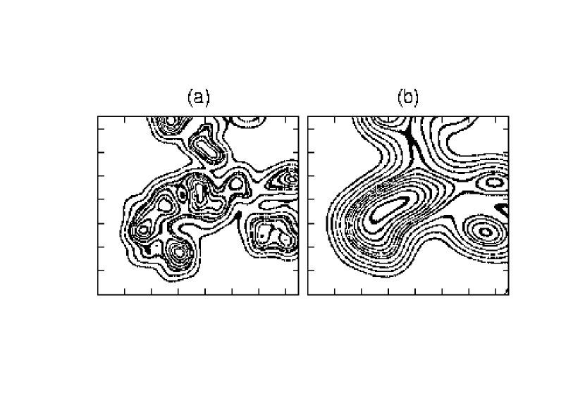
Figure 2: A slice along the $z=0$ plane showing density contours of part of a fractal with $D_{f}=2.6$, calculated by using equation (1) with (a) $\sigma=\sigma_{opt}$ and (b) $\sigma=2\sigma_{opt}$.

is an example of the appearance of the density field resulting from applying equation (1) to a fractal with $D_{f}=2.6$. Each map is a slice along the $z=0$ plane showing density contours of a part of the three-dimensional density field. The left-side map (a) was generated with $\sigma=\sigma_{opt}$, whereas the right-side map (b) is exactly the same region but generated with $\sigma=2\sigma_{opt}$. Clearly we see that as $\sigma$ increases some density peaks tend to blend with other peaks forming smoother regions. Several tests showed that the properties studied in this work do not depend (within the error bars) on the exact value of $\sigma$ as long as this value is of the order of $\sigma_{opt}$. This value can be different from fractal to fractal but always was of order $\sim 10^{-2}R_{f}$.

In Figure 3

Figure 3: The density pdf calculated by using a gaussian kernel with $\sigma=\sigma_{opt}$, for different values of fractal dimension: $D_{f}=3$ (dotted line), $D_{f}=2.6$ (solid line), $D_{f}=2.3$ (long dashed line), and $D_{f}=2.0$ (short dashed line).

we show the normalized density pdf calculated (with $\sigma=\sigma_{opt}$) for the fractals with dimensions $D_{f}=3$, $D_{f}=2.6$, $D_{f}=2.3$, and $D_{f}=2.0$. The long tails at low densities come from the sampling in or close to the edge and/or the voids existing in the fractal clouds. The maximum of the distribution moves toward higher density values as $D_{f}$ decreases according to the relation $\rho_{max}\varpropto R^{-(3-D_{f})}$ for $R\sim constant$, from $\rho_{max}/\rho_{f}=1$ for $D_{f}=3$ to $\rho_{max}/\rho_{f}\simeq 10$ for $D_{f}=2.0$. There is always a turn over in the pdf, decaying rapidly at densities just after the maximum.

The density pdf is a fundamental statistical quantity characterizing the structure of a given medium. Despite the pdf being a one-point statistic containing no spatial information, the knowledge of this function is a fundamental step prior to the analysis of the star formation process and the stellar initial mass function (e.g. Padoan & Nordlund, 2002; Scalo et al., 1998). The problem is that the density pdf cannot be directly measured in the ISM, instead the column density pdf is measured. Ostriker et al. (2001) used three-dimensional numerical simulations of isothermal magnetohydrodynamic turbulence to compare the resulting density field with the column densities, finding that both distributions had very similar shapes (approximately lognormal). Also Fischera & Dopita (2004) showed that lognormal density distributions produce lognormal column density pdf’s. However, column density observations cannot always be fitted to lognormal distributions and can show extended tails (Blitz & Williams, 1997) or simply a power law behavior (Heiles & Troland, 2005).

The suggestion that the density pdf in the ISM should be consistent with a lognormal distribution comes from the central limit theorem applied to a multiplicative hierarchical density field (Vazquez-Semadeni, 1994). Several authors have found that the density pdf of turbulent gas should exhibit a roughly lognormal distribution under a wide range of physical conditions (Ballesteros-Paredes, 2004; Elmegreen & Scalo, 2004, and references there in). For a polytropic gas (where $P\varpropto\rho^{n}$) the shape of the pdf depends on the effective polytropic index $n$. If the gas is isothermal ($n=1$) the pdf is lognormal (Vazquez-Semadeni, 1994) but extended tails can develop at high or low densities if $n\neq 1$ (Passot & Vazquez-Semadeni, 1998; Scalo et al., 1998; Ostriker et al., 2001), and the departure from a lognormal is larger at higher Mach numbers (Beresnyak et al., 2005). The one-dimensional simulations of highly compressible turbulence of Passot & Vazquez-Semadeni (1998) showed that a power law tail develops at relatively high densities if $n<1$ and at low densities if $n>1$. Their results for $n>1$ and high Mach numbers resemble the pdf’s we showed in Figure 3.

The situation becomes more complicated if we try to understand the dependence of the density pdf on the physical mechanisms acting in the turbulent medium. Li et al. (2003) found that shocks sweep up the gas producing low density regions and pdf’s skewed to low densities, but self-gravity tends to collect the gas producing pdf’s with positive skewness. The presence of a magnetic field has, however, very little effect on the density pdf (Passot & Vazquez-Semadeni, 2003). The large-scale simulations performed by Wada & Norman (2001) showed a roughly constant pdf shape (lognormal at high densities and normal at low densities) regardless of whether star formation is considered or not in the simulation. Slyz et al. (2005) arrive to very different conclusions, finding that the pdf does depend sensitively on the simulated physics. Their pdf is consistent with a lognormal function only for the runs where neither supernova feedback nor self-gravity are implemented. With the addition of self-gravity the pdf approaches a power law at high densities, but it becomes markedly bimodal when supernova feedback is included (with or without self-gravity).

4 Clump definition

Starting from the three-dimensional density field calculated by applying equation (1) to the generated fractals, we want to study the properties of the resulting “density condensations”. We will call these regions “clumps” to differentiate it from the whole fractal structure, which we could associate with a giant molecular cloud. Actually this denomination is arbitrary, firstly because there are no precise definitions of terms like “cloud”, “clump”, or “core” (Larson, 2003), and secondly because here we can not speak about an absolute spatial scale but about self-similar structures inside a region of size $R_{f}$. Different schemes can be adopted in defining a clump. For example, the algorithm called GAUSSCLUMPS (Stutzki & Gusten, 1990) uses a least squares fitting procedure to decompose iteratively the emission in one or more gaussian clumps, instead CLUMPFIND (Williams et al., 1994) associates each local emission peak and the neighboring pixels with only one clump (similar to the usual eye-inspection procedure). In both cases, the implicit assumption that the radial velocity coordinate can be replaced by the radial distance is made, but this assumption is not necessarily always satisfied (Ostriker et al., 2001). In our case, this problem does not exist because we are using three spatial coordinates and density values, but we have to keep in mind that comparison with observations may not be done directly. For simplicity, we have chosen to associate each peak in density with one clump (in the same way that CLUMPFIND does). Once we have identified a peak we determine the mass of the clump by integrating the density field over the neighboring region. In order to proceed with the calculation we need to place a grid over the volume occupied by the fractal cloud. The size of the cell was chosen to equal de value of $\sigma_{opt}$, that is, to equal the resolution with which the density field was generated. Since $\sigma_{opt}/R_{f}$ was always of order of $10^{-2}$ or less, there were always $\sim 10^{6}$ cells or more over the fractal.

An important aspect to consider when defining a clump is the noise present in the data, whether it be observational or numerically simulated. Usually the problem is approached by defining a free parameter such that fluctuations of the order of (or smaller than) this parameter are not considered as clumps. For example, in the algorithm CLUMPFIND this parameter is the step between two successive contours, in the simulations of Gammie et al. (2003) is their smoothing length, and in this work it is the parameter $\sigma$ used in equation (1) to generate the density field. Another very important point is to define the boundary of the cloud, i.e., to define which neighboring region “belongs” to the clump and which not. Again the usual approach is to introduce an additional parameter: the threshold density (or emission). Thus, a common definition for clump in literature is all the pixels around a maximum in density with values greater than some predefined threshold value. The algorithm we have constructed to identify clumps works in the following manner. First, it associates the pixel with highest density value to the first clump. Then it takes the pixel whose density value is just below the highest, and if this pixel is neighbor of the first one then it “belongs” to the first clump. If by the contrary this pixel is isolated then it is labeled as the first pixel of the second clump. All the pixels are explored successively in decreasing order of density in the same way: if a pixel is contiguous to the boundary of some existing clump then it belongs to this clump, otherwise it belongs to a new clump. This procedure continues until some threshold density is reached.

When this threshold is relatively low there can be an additional problem: two (or more) peaks in density may be present in the region above the threshold, and we have to “decide” to which of the available peaks the pixels that are contiguous to two or more boundaries should be assigned to. The criterion normally used is purely geometric: each “ambiguous” pixel is assigned to the clump with the closest peak (just like CLUMPFIND does). However, we should ask ourselves whether different criteria could be used to assign “membership” in a more “suitable” way. An alternative criterion could be to assign each ambiguous pixel to the clump with highest “gravitational potential”. We have tested the former criterion by estimating the potential (at the moment of considering the $i$-th pixel) as the current clump mass ($M_{i}$) divided by the peak-pixel distance ($d_{i}$). Then, each ambiguous pixel is attached to the clump with higher $M_{i}/d_{i}$ value rather than to the clump with higher $1/d_{i}$ value (i.e., smaller distance). If the threshold density is close to the maximum density values for two neighbor clumps, then the clumps will be physically separated and any criteria for ambiguous pixels will yield the same result. As threshold density ($\rho_{th}$) decreases the adjacent surface between two neighbor clumps increases and therefore the effect of different criteria becomes more important. As an example, Figure 4

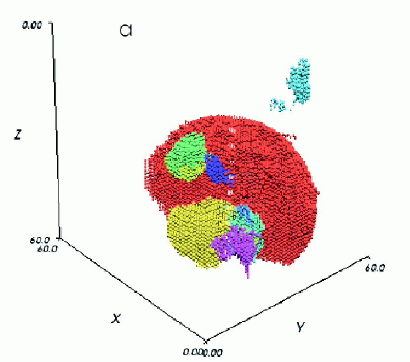
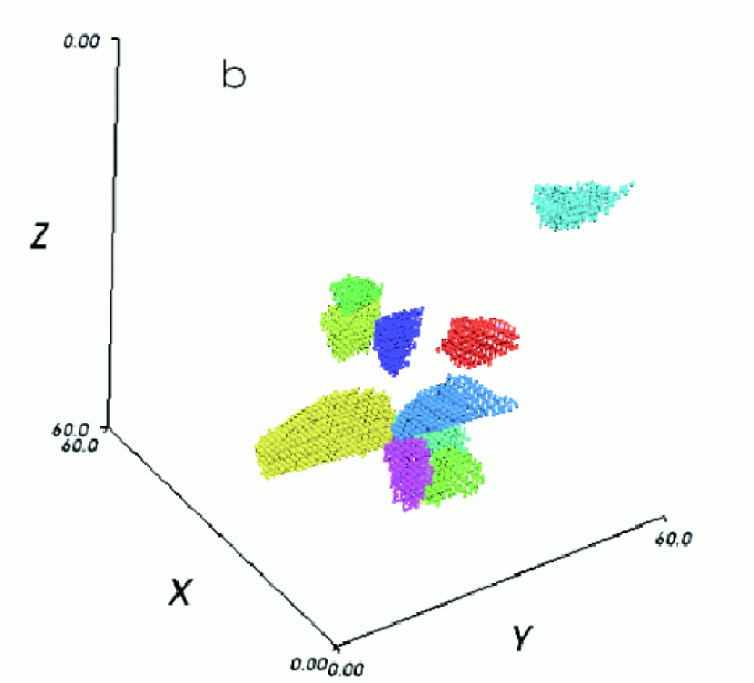
Figure 4: Images of the clumps resulting (each one with a different color) from ten density peaks when $\rho_{th}=0$, for the first random fractal generated with $D_{f}=2.6$, using (a) the criterion “potential” and (b) the criterion “distance” (see text). The coordinates are the pixel coordinates.

shows ten of the resulting clumps when $\rho_{th}=0$ for the first random fractal we simulated with $D_{f}=2.6$ and for both criteria mentioned above. The criterion of distance tends to produce more symmetrical (and similar in shape) clumps, and in this case the clump volume distribution relates directly with the peak-peak distance distribution between neighbors, which is random for the fractal sets we are generating. This degenerates into a clump mass distribution narrower than for the criterion of potential, as can be seen in Figure 5a

Figure 5: The clump mass spectra for ten random fractals with $D_{f}=2.6$ when using the criterion of potential (solid line histograms) and the criterion of distance (dashed line histograms). (a) All the cloud gas is forming clumps and (b) only 10% of the cloud gas is in the form of clumps.

where the number of clumps per logarithmic mass interval (normalized to the total number of clumps) $N_{cl}/N_{tot}$ has been plotted as a function of the clump mass in units of the total mass ($M_{cl}/M_{f}$). Thus, the same cloud density field and therefore the same number of clumps yields very different mass distributions only changing the criterion with which the low density pixels are distributed. The differences are amplified simply because we are artificially creating clumps from extremely low density material which typically remains in the form of inter-clump gas. The clumps obtained by distributing all the cloud mass in clumps are far from looking similar to those obtained from observations: there are no observed clouds formed only by clumps without inter-clump material. We have verified that in more realistic situations when $\rho_{th}>0$, i.e. when an inter-clump density is defined, clumps resulting from applying different criteria and therefore their global properties (such as mass and size distributions) gradually begin to converge as $\rho_{th}$ increases. In fact, when only 10% of the cloud mass is forming clumps both criteria for selection of clumps yield very similar mass distributions (see Figure 5b). In other words, when we only see the dense “cores” the method of distributing low density pixels does not play any important role. In section 5.3 we analyze the effect of the threshold density on the global clump properties in order to understand how these properties are modified in clouds observed with different degrees of sensitivity and contrast.

We have tested several different criteria for clump selection but the global results always are similar to one or another of the two criteria above, depending on whether peak-pixel distance or clump mass is the dominant factor in the criterion applied. Here we have chosen to discuss in detail the properties resulting when using the (physically inspired) criterion of the “potential”. When considering the clump mass for deciding about ambiguous pixels this criterion takes into account in some way the underlying density pdf, which depends on the cloud fractal dimension (section 3). The properties we derived by using the criterion of distance map the random distribution of distances between neighbor density peaks rather than of intrinsic density structure. However, the sensitivity of the cloud properties, both simulated and observed, to different clump selection criteria is an important problem that must be addressed in future works.

5 Properties of fractal clouds

We have defined each clump as all the mass enclosed from the density peak to a threshold density. For convenience, we have chosen the simplest way to define this threshold: a constant value such that a given ratio, $\epsilon$, of the total mass in clumps to the total cloud mass is obtained. If $\epsilon=1$ the number of clumps formed will equal the number of density peaks, which is given by the three-dimensional density field (i.e., by $D_{f}$) and it does not depend on the clump selection criterion. Low $D_{f}$ values imply more fragmented clouds (higher number of clumps). But additionally at low $\epsilon$ values some peaks could be below the threshold density and then there could be a lesser number of clumps. Table 1 shows the average number of clumps (per simulation) obtained for the results we discuss in this work. We first discuss the results for $\epsilon=1$ and in section 5.3 we analyze the effect of changing the threshold density.

Table 1: Average number of clumps formed per fractal cloud

$D_{f}$	$\epsilon=1$	$\epsilon=0.5$	$\epsilon=0.25$	$\epsilon=0.1$
2.0	764.6	764.6	737.6	556.8
2.1	620.6	620.6	592.7	469.3
2.2	531.1	531.1	514.6	410.2
2.3	427.5	427.2	412.5	316.8
2.4	343.9	343.4	328.7	244.2
2.5	262.1	262.0	243.5	175.4
2.6	189.8	189.5	175.0	133.6
3.0	118.0	116.4	106.1	80.4

5.1 Masses, densities, and sizes

Generally the resulting clump shapes do not have a regular geometry (see the examples in Figures 2 and 4). Under these circumstances it is not easy to define a clump “radius”, so we have defined a characteristic radius simply as the cubic root of the clump volume. Figure 6 shows

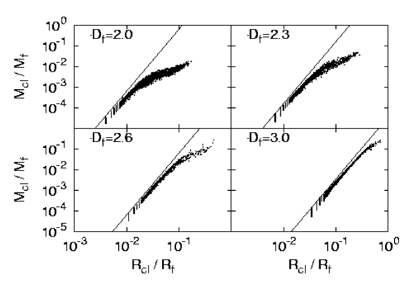
Figure 6: Clump mass, $M_{cl}$, as a function of radius, $R_{cl}$, for the labeled values of fractal dimension $D_{f}$. The solid line corresponds to the constant density case.

the mass of the clumps ($M_{cl}$) as a function of the radius ($R_{cl}$) for four different values of the fractal dimension ($D_{f}=2.0$, $2.3$, $2.6$, and $3.0$). The corresponding average densities ($\rho_{cl}$) are shown in Figure 7.

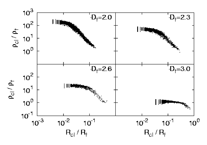
Figure 7: The average clump density, $\rho_{cl}$, as a function of the radius, $R_{cl}$, for the labeled values of fractal dimension $D_{f}$.

The range of possible sizes depends in principle on the fractal dimension (that determines the way in which fragmentation occurs) and on the number of levels (that determines how many fragmentations occur). When generating the fractal structure the smallest fragments have radii $R_{min}/R_{f}=(1/N^{H})^{1/D_{f}}$. Computational limitations prevented us from using more than $H=9$ levels, so the smallest structures have sizes $\sim 7\times 10^{-3}R_{f}$ for $D_{f}=2.0$ and $\sim 4\times 10^{-2}R_{f}$ for $D_{f}=3.0$. The size range obtained is more or less between these minimum values and the theoretical maximum $R_{cl}/R_{f}=1$. Generally speaking, mass does not obey a power law with size of the type $M_{cl}\varpropto R_{cl}^{\gamma}$ along all the size range (Figure 6), and therefore neither density obeys the corresponding $\rho_{cl}\varpropto R_{cl}^{\gamma-3}$ (Figure 7). We would expect $\gamma=D_{f}$ in the case of random sampling throughout the hierarchy (section 2), but what we see is $\gamma\simeq 3$ (i.e., $\rho\simeq constant$) at small sizes and then $\gamma$ gradually decreases as $R_{cl}$ increases. For comparison, we show in Figure 6 the lines corresponding to $\rho_{cl}=constant$. The decrease in the $\gamma$ value is more abrupt for low $D_{f}$ values, while for the extreme case $D_{f}=3$ we get $\gamma\simeq 3$ along almost the full size range. For $D_{f}=3$ the range in density values is very narrow and close to $\rho_{cl}/\rho_{f}=1$ (as expected), but for lower $D_{f}$ values the density range increases and tends to higher values (Figure 7). The latter situation corresponds to more fragmented structures with small dense clumps separated by large low density regions.

An empirical power law scaling relation with $\gamma\simeq 2$ was first pointed out by Larson (1981) for molecular cloud complexes (in the range $0.1\lesssim R\lesssim 100\ pc$ and $1\lesssim M\lesssim 10^{6}\ M_{\sun}$), although it has been argued that this result could be simply an artifact due to observational limitations that strongly constraint the range of observed column densities (Scalo, 1990). This power law behavior has been generally interpreted as a consequence of the mechanical equilibrium in self-gravitating, turbulent molecular clouds, but also very different physical processes can reproduce this type of relations (see Elmegreen & Scalo, 2004, and references therein). From the observational point of view, the problem is that many studies show a weak or scatter-dominated correlation. Moreover, comparing different observational studies is always difficult because of the existing variety in observational techniques and criteria used to define or derive properties such as mass, radius, etc. Elmegreen & Falgarone (1996) used several surveys from the literature and found $\gamma\simeq 2.35$, which was interpreted as a direct consequence of an underlying fractal structure with $D_{f}\simeq 2.35$. However, this result only emerges when the clouds and clumps from many regions are analyzed as an ensemble, while the power laws measured in individual regions have $\gamma\simeq 2.4-3.7$, with values $\gtrsim 3$ being typical. Reid & Wilson (2005) found $\gamma\simeq 1.5-2.1$ in the range $1\lesssim M\lesssim 10^{3}\ M_{\sun}$, whereas Heithausen et al. (1998) found a steeper slope ($\gamma\simeq 2.3$) in the range $10^{-4}\lesssim M\lesssim 10^{2}\ M_{\sun}$. Caselli & Myers (1995) have already observed a change in the power law slope between large mass and low mass cores in Orion A and B. Falgarone et al. (2004) have argued that, in spite of the large scatter, it seems that $\gamma\simeq 2$ better characterizes large scale structures and $\gamma\simeq 2.3$ the small scale ones.

Our results seem to favor a change in the slope of the $M_{cl}-R_{cl}$ relation, although less steep as $D_{f}$ increases. The manner in which $M_{cl}$ increases with $R_{cl}$ is determined by the density profile of the clumps. For flat density profiles, $\rho(x,y,z)=constant$, we would expect to see $M_{cl}=\int_{V_{cl}}\rho(x,y,z)dV\sim R_{cl}^{3}$. For extremely narrow density profiles of the form $\rho(x,y,z)=\rho_{0}\delta(x_{0},y_{0},z_{0})$, being $\delta$ the delta of Dirac and $\rho_{0}$ the density value of a little region of volume $V_{0}$ around $(x_{0},y_{0},z_{0})$, we would have $M_{cl}=\int_{V_{cl}}\rho(x,y,z)dV=\rho_{0}V_{0}=constant$. The observed behavior is directly related to a gradual change in clump density profiles from very flat shapes at small sizes to narrower ones at large sizes. As an example, Figure 8

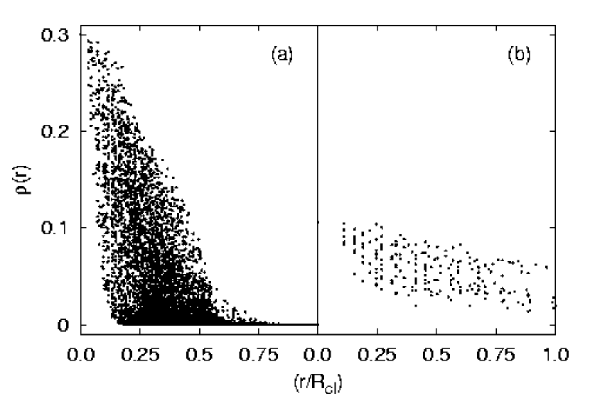
Figure 8: The density of each pixel as a function of its distance (in units of the clump size) from the pixel having the maximum density value, for (a) a large and (b) a smaller clump in one of the fractals with $D_{f}=2.6$.

shows density profiles for two different clumps in one of the fractals with $D_{f}=2.6$. We have plotted the density of each pixel as a function of its distance from the pixel having the maximum density value. The scatter in these plots is due to the asymmetry of the clump shapes. The figure labeled (a) corresponds to a clump $\sim 40$ times more massive and $\sim 10$ times larger than the clump in (b), and the characteristics mentioned before can readily be appreciated. This is an interesting property of the fractal density distribution we are generating, in which large clumps are the result of the “agglomeration” (through a gaussian convolution with equation 1) of particles in the last level of hierarchy in the original fractal. Its consequences for the derived clump properties will be discussed in section 5.3.

5.2 Clump mass and size spectra

The clump mass spectra (number of clumps $N_{cl}$ per logarithmic mass interval) for different $D_{f}$ values are shown in Figure 9.

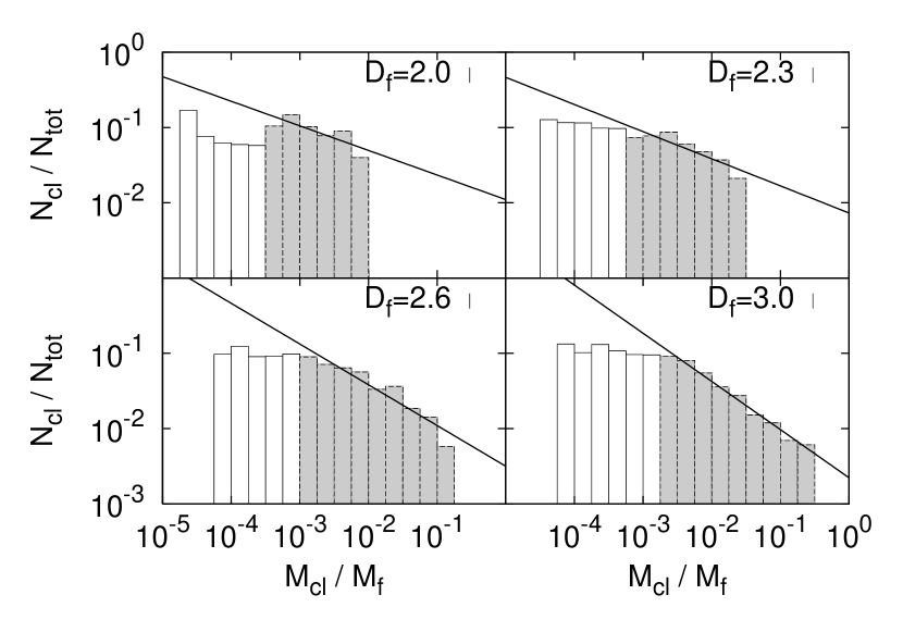
Figure 9: The clump mass spectra for the labeled values of fractal dimension $D_{f}$. The filled histograms indicate the mass range for clumps having a volume larger than $\sim 10$ pixels, and the solid lines are the best fits in these ranges.

The filled histograms indicate the ranges corresponding to clumps having a volume larger than $\sim 10$ pixels, which were the ranges where a power law-like behavior was observed: $N_{cl}\varpropto M_{cl}^{-\alpha_{M}}$. The best fits in these ranges (solid lines) show clearly steeper slopes as the fractal dimension increases. The fits yielded: $\alpha_{M}\simeq 0.33\pm 0.12$ for $D_{f}=2.0$, $\alpha_{M}\simeq 0.36\pm 0.08$ for $D_{f}=2.3$, $\alpha_{M}\simeq 0.54\pm 0.06$ for $D_{f}=2.6$, and $\alpha_{M}\simeq 0.64\pm 0.03$ for $D_{f}=3.0$. The mass spectra become flatter in the low mass range. We have to point out that we are not saying that the intrinsic mass spectra are actually power laws, but we are simply characterizing the spectra with the functional form commonly used by observers in order to better compare these results. From simple random sampling through the hierarchy we would expect $\alpha_{M}=1$ (see section 2), but we already mentioned that if double counting is avoided and/or random blending is taken into account the observed index should be less than this value. Clouds with high fractal dimensions are less fragmented than low fractal dimension clouds. They have a relatively small number of clumps but, on average, these clumps have larger sizes and higher masses. As $D_{f}$ increases clouds tend to be more homogeneous, and that is why the average clump densities are always close to the whole cloud density (Figure 7). Additionally, the volume in clumps approach the total cloud volume as $D_{f}$ increases (the filling factor tends to 1 as $D_{f}$ tends to 3), and the clumps are relatively close to each other. On the opposite, at very low fractal dimensions the high density clumps are separated by low density (or empty at all) regions. Ultimately, low fractal dimension clouds distribute their material more homogeneously between the larger number of well differentiated clumps. At high fractal dimensions a greater amount of “ambiguous” material is assigned to massive clumps leaving a higher number of small clumps. It is for this reason that the mass spectrum slope is flatter for small $D_{f}$ values.

The clump size spectra (per logarithmic size interval) are shown in Figure 10

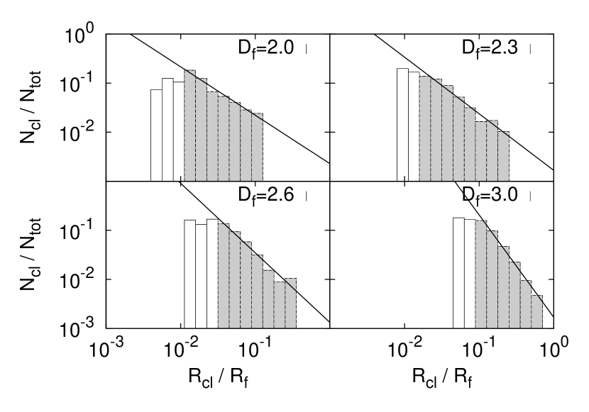
Figure 10: The clump size spectra for the labeled values of fractal dimension $D_{f}$. The filled histograms indicate the size range for clumps having a volume larger than $\sim 10$ pixels, and the solid lines are the best fits in these ranges.

for the same fractal dimension values as in Figure 9. Again, the filled histograms indicate the ranges for clumps larger than $\sim 10$ pixels, and the solid lines are the best fits in these ranges. The near-power law behavior $N_{cl}\varpropto R_{cl}^{-\alpha_{R}}$ becomes steeper as $D_{f}$ increases, as the fitted slopes show: $\alpha_{R}\simeq 0.99\pm 0.07$ for $D_{f}=2.0$, $\alpha_{R}\simeq 1.15\pm 0.08$ for $D_{f}=2.3$, $\alpha_{R}\simeq 1.42\pm 0.13$ for $D_{f}=2.6$, and $\alpha_{R}\simeq 2.09\pm 0.08$ for $D_{f}=3.0$. As for the mass spectra, the final distribution is flatter than the random sampling slope which is $\alpha_{R}=D_{f}$ and, as before, the relative importance of the clump selection criterion when applied to more or less fragmented clouds causes the differences in the derived slopes for different $D_{f}$ values. It is interesting to mention that if mass and radius could be related as $M_{cl}\varpropto R_{cl}^{\gamma}$ then the power law indices satisfy a relationship of the form $\alpha_{R}=\gamma\alpha_{M}$. For the random sampling case we have $\gamma=D_{f}$, $\alpha_{M}=1$, and then $\alpha_{R}=D_{f}$, as shown in section 2; but our results do not show a scale relation between mass and radius ($\gamma\neq constant$, see Figure 6) and therefore this kind of simple relations cannot be found.

The power-law behavior obtained for both the mass and size distributions are in general consistent with observations. However, the detailed comparison is extremely difficult considering the great diversity of results reported in the literature and considering that no clear relationship has been observed between the mass or size distributions and the mean physical properties of the ISM. The most accepted view is a nearly constant mass and size distributions throughout a large range of scales, according to a fractal picture for the ISM (see, for instance, the reviews of Evans, 1999; Williams et al., 2000; Falgarone et al., 2004, and references therein). When a sufficiently large number of clumps is considered, galactic surveys indicate that on average $\alpha_{M}\sim 0.8$ in the range $1\lesssim M\lesssim 10^{7}\ M_{\sun}$ and $\alpha_{R}\sim 2.3$ in the range $0.1\lesssim R\lesssim 10^{2}\ pc$ (Elmegreen & Falgarone, 1996), and these results seem to depend very little, if any, on physical properties like selfgravitation or the degree of star formation activity (Simon et al., 2001). The extension at lower masses and sizes yields $0.6\lesssim\alpha_{M}\lesssim 0.8$ for $10^{-4}\lesssim M\lesssim 10^{3}\ M_{\sun}$ and $\alpha_{R}\sim 2.0\pm 0.2$ for $10^{-2}\lesssim R\lesssim 1\ pc$ (Heithausen et al., 1998; Kramer et al., 1998). The mass and size distributions obtained here have indices in the range $0.3\lesssim\alpha_{M}\lesssim 0.6$ and $1.0\lesssim\alpha_{R}\lesssim 2.1$ for $2\leq D_{f}\leq 3$. If we assume $D_{f}\simeq 2.6$ then $\alpha_{M}\sim 0.5$ and $\alpha_{R}\sim 1.4$, a little lower but in gross agreement with mean observed values. Steeper slopes can be obtained only for $D_{f}>2.6$. These results seem to favor the idea that the ISM has a fractal dimension higher than the usually assumed value $D_{f}\simeq 2.3$ (Sánchez et al., 2005). However, the situation is far from being totally understood. The mass distribution slopes may be as steep as, for example, $\alpha_{M}\simeq 1.1$ for filamentary clumps in Orion A molecular cloud (Nagahama et al., 1998) or as flat as $\alpha_{M}\simeq 0.3$ for the Rosette molecular cloud (Williams et al., 1994), not being obvious whether these observations reveal real differences from region to region. Schneider & Brooks (2004) have demonstrated that the derived properties differ significantly when using different clump identification methods. The algorithm GAUSSCLUMPS (Stutzki & Gusten, 1990) is able to separate blended clumps, although tends to introduce spurious features if the structures do not have gaussian shapes. On the other hand, CLUMPFIND (Williams et al., 1994) is able to find arbitrarily shaped clumps but it does not detect less massive clumps which are blended with others. Thus, generally speaking, one would expect steeper mass distributions for GAUSSCLUMPS than for CLUMPFIND (Schneider & Brooks, 2004), but error bars are usually large and this behavior cannot be appreciated (Mookerjea et al., 2004). The situation is worst for the size distributions because clump sizes are quantities more difficult to estimate in a robust manner, particularly for small, low intensity objects close to the resolution limits (Elmegreen & Falgarone, 1996; Heithausen et al., 1998).

5.3 Dependence on the threshold density

The previous results refer to the case $\epsilon=1$. A smaller $\epsilon$ value implies that not all the cloud complex mass has formed clumps. We have simulated this effect by considering a (constant) threshold density such that pixels with densities below this threshold value are not taken into account when constructing clumps. In principle, $\epsilon$ could be related to observational limitations, because smaller $\epsilon$ values arise from the fact that there is a threshold density level for observations. Also we could associate it with the actual mass fraction in clumps, being the rest of the mass kept in a diffuse interclump medium (Blitz & Stark, 1986; Wood et al., 2005). In such a case $\epsilon$ could be around $\sim 0.9$ or even much less (Blitz & Stark, 1986; Pagani, 1998). One possibility is to assume that a fixed fraction of clump masses will form dense prestellar cores and then $\epsilon\sim 0.1$ (if we assume a star formation efficiency $\sim 10\%$), although obviously the formation of gravitationally bounded cores is a process more complex than this. The threshold densities we discuss here have been chosen to obtain the following $\epsilon$ values: $0.5$, $0.25$, and $0.1$, and all the clump properties were recalculated.

For $\epsilon\leq 0.5$ the mass-radius relations for the clumps correspond to the $\rho_{cl}=constant$ case. The range of masses decreases, which is not a surprising result since part of the clumps mass has been removed, but additionally the mass spectra behavior modifies in an interesting way: as $\epsilon$ decreases the slope in the power law range becomes steeper. The mass spectra for the same fractal dimensions as before but for $\epsilon=0.1$ are shown in Figure 11.

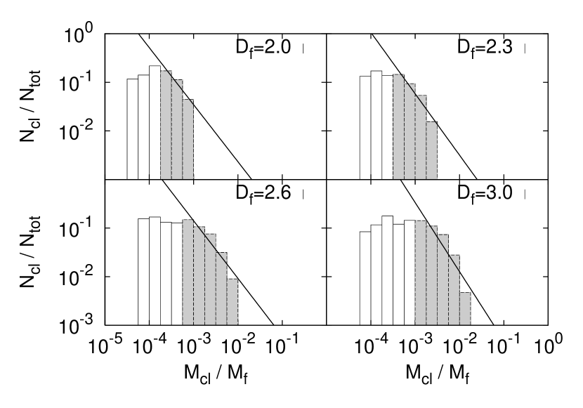
Figure 11: The same as in Figure 9, but for $\epsilon=0.1$.

The same general behavior is kept (a power law at high masses with a flattening at low masses) but the slope values changed notoriously. For example, for the case $D_{f}=2.6$ the index $\alpha_{M}$ increased from $0.54\pm 0.06$ ($\epsilon=1$) to $1.19\pm 0.20$ ($\epsilon=0.1$). We have summarized all the obtained mass spectra by plotting in Figure 12

Figure 12: The power law index $\alpha_{M}$ as a function of the fractal dimension $D_{f}$ for three different values of $\epsilon$: $1.0$ (circles), $0.25$ (squares), and $0.1$ (triangles). The bars on the data are the standard deviations of the best fits. The results for $\epsilon=0.5$ are very close to those for $\epsilon=1$ and are not shown for the sake of clarity.

the power law slope $\alpha_{M}$ as a function of the fractal dimension $D_{f}$ for three different values of $\epsilon$ ($1.0$, $0.25$, and $0.1$). The result for $\epsilon=0.5$ is so close to the result for $\epsilon=1$ that it is not shown for simplicity. As already mentioned, the general behavior is an increase of $\alpha_{M}$ (steeper slopes) as $D_{f}$ increases, but also $\alpha_{M}$ increases as $\epsilon$ decreases. In spite of the bar sizes, Figure 12 allows us to quantify approximately the dependence of $\alpha_{M}$ on both $D_{f}$ and $\epsilon$. Part of the uncertainty comes from fitting power law functions to distributions that depart from this behavior.

Concerning the clump size spectra, when $\epsilon=0.5$ the size range decreases in such a way that a clear power law behavior is not seen, mainly at low fractal dimensions. However, we have followed the objective procedure of fitting a power law for structures bigger than $\sim 10$ pixels, and we obtained flatter distributions. For example, for $D_{f}=2.6$ we have that $\alpha_{R}$ decreased from $1.42\pm 0.13$ ($\epsilon=1$) to $0.92\pm 0.20$ ($\epsilon=0.5$). The obtained power law slopes $\alpha_{R}$ as a function of the fractal dimensions $D_{f}$ for $\epsilon=1$ and $\epsilon=0.5$ are shown in Figure 13.

Figure 13: The power law index $\alpha_{R}$ as a function of the fractal dimension $D_{f}$ for two different values of $\epsilon$: $1.0$ (circles), and $0.5$ (squares). The bars on the data are the standard deviations of the best fits.

For smaller $\epsilon$ values the size ranges were so narrow that fits could not be done and/or standard deviation bars were extremely large. The power law index $\alpha_{R}$ increases as $D_{f}$ increases, but now we have that $\alpha_{R}$ also decreases when $\epsilon$ decreases, in opposite to the mass spectra.

The trend of steeper mass distributions for higher threshold densities (smaller $\epsilon$ values) was seen by Elmegreen (2002) in his model of fractal brownian motion clouds, although he only simulated clouds with constant fractal dimension ($D_{f}\simeq 2.75$ on average). It is not easy to understand the dependence of $\alpha_{M}$ and $\alpha_{R}$ on $\epsilon$, but as in the work of Elmegreen (2002) it has to do with changes in the density profiles between the smallest and largest clumps. In section 5.1 we argued that density profiles of small clumps are flatter than those in large, massive clumps (which have lesser average density). Large clumps have narrow, tall profiles with long tails at low densities (see the example in Figure 8). Then, when the threshold density is increased, both sizes and masses decrease, but in different ways. Large clumps decrease their sizes in a higher proportion than the small ones, because of the long tails. Thus, the size distribution flattens because the proportion of high radius clumps increases (relative to the small ones). On the opposite, there is not too much mass below the low density tails and then the masses of large clumps decrease in a lower proportion than for smaller clumps. Therefore, when the threshold increases the proportion of high mass clumps decreases and the mass distribution becomes steeper.

We have seen that for more realistic $\epsilon$ values (i.e., $\epsilon<1$) we get steeper mass functions and flatter size functions. The case $\epsilon=0.5$ and $D_{f}=2.6$ yields $0.7\lesssim\alpha_{R}\lesssim 1.1$, which is much flatter than the average observed in molecular clouds but remarkably similar to the size distribution recently observed for HI clouds in the LMC (Kim et al., 2005). Additionally, according to our results, molecular cloud complexes with $D_{f}=2.6$ will have mass functions $\alpha_{M}\sim 1.2\pm 0.2$ when $\epsilon=0.1$, very close to the value $1.35$ of Salpeter (1955). In fact, the observed mass spectrum of dense cores seems to have a form significantly different from molecular clumps, with the slope relatively flatter ($\alpha_{M}\simeq 0.5$) at low masses and steeper ($\alpha_{M}\simeq 1.5$) at high masses (Motte et al., 1998; Reid & Wilson, 2005). Our results reproduce this behavior, we clearly appreciate (in spite of the large standard deviation bars) a systematically steeper mass function at high masses as $\epsilon$ decreases. This is a very conspicuous result: the denser regions in the fractal cloud complex have a Salpeter-like mass function steeper than the mass function of the whole complex. An interesting point is that the mass distribution slope for $\epsilon=0.1$ is near to the Salpeter value (within the error bars) in a wide range of fractal dimension values ($2.0\lesssim D_{f}\lesssim 2.6$). It seems that the information about the fractal density structure is lost when we only see the central dense “cores”. The results we showed in this section suggest a direct link between cloud structure and star formation.

6 CONCLUSIONS

In this work we have studied the relation between the physical properties of interstellar cloud complexes and their underlying fractal structure. For a better understanding of this relationship we have used a simple algorithm that generates fractal clouds with fractal dimensions well defined in a wide range of space scales. We have not considered physical processes to generate either the fractal structure or the embedded clumps. In any case, the exact physical nature of clumps still remains uncertain; whether they are temporary density fluctuations caused by supersonic turbulence or more stable structures confined by the interclump medium (Williams et al., 2000). The simple approach given here allows us to analyze in an empirical way the dependence of the ISM properties on both the fractal dimension and the threshold density.

We observe that the number of clumps (as given by the number of relative maxima of density) depends only on the density structure of the whole cloud, which can be associated to a single parameter: the fractal dimension. However, when the whole mass of the cloud is distributed amongst the different clumps (i.e., $\epsilon=1$), the mass and size distributions are highly dependent on the clump defining criterium chosen. On the other hand, as the fraction of the total mass in the form of clumps ($\epsilon$) decreases the mass and size distributions become similar for different criteria of clump selection, i.e., when only the “cores” of the “clumps” are selected their distributions in mass and radius are not dependent on the selection criteria. This fact leads to an interesting conclusion: the “cores” mass and size distributions are only driven by the fractal dimension of the clouds. A true molecular cloud contains relatively empty voids, dense cores, as well as rarefied intercloud material (Gammie et al., 2003), which looks like more similar to the distributions of cores obtained for $\epsilon=0.1$ than the clumps distribution for $\epsilon=1$.

In general, the masses and radii of the resulting clumps do not fulfill simple power law relations of the type $M_{cl}\varpropto R_{cl}^{\gamma}$ along all the size range. We obtain that $\gamma\simeq 3$ at small sizes and $\gamma<3$ at larger sizes with the exact behavior depending on the fractal dimension. The reason for the departure from a power law has to do with the differences in the density profiles between the smallest and largest clumps: small clumps have flat density profiles whereas large clumps have narrow and tall profiles with long tails at low densities.

The number of clumps per logarithmic interval of mass (or size) can be fitted to a power law function $N_{cl}\varpropto M_{cl}^{-\alpha_{M}}$ (or $N_{cl}\varpropto R_{cl}^{-\alpha_{R}}$) in a certain range of mass (or size). The indices $\alpha_{M}$ and $\alpha_{R}$ depend both on the fractal dimension ($D_{f}$) and on the fraction of the total mass in the form of clumps ($\epsilon$). Our main results are summarized in Figures 12 and 13, and they refer to the dependence of the clump mass and size spectra on both $D_{f}$ and $\epsilon$. For the case $\epsilon=1$ we obtain that as $D_{f}$ increases from $2$ to $3$ $\alpha_{M}$ increases from $\sim 0.3$ to $\sim 0.6$ whereas $\alpha_{R}$ increases from $\sim 1.0$ to $\sim 2.1$. Rough comparison with observations suggests that $D_{f}\simeq 2.6$ is consistent with the average properties of the ISM. This value for the ISM fractal dimension is in agreement with previous results based on the fractal dimension measured on the projected images of clouds (Sánchez et al., 2005). On the other hand, as $\epsilon$ decreases $\alpha_{M}$ increases and $\alpha_{R}$ decreases. For the case $\epsilon=0.1$ (only $10\%$ of the complex mass is in the form of dense clumps) we obtain $\alpha_{M}\simeq 1.2$ for $D_{f}=2.6$, a value remarkably similar to the Salpeter (1955) value, suggesting that the stellar initial mass function could be intimately related to the internal structure of molecular cloud complexes.

In summary, we have derived the properties of fractal cloud complexes, no mattering the physical processes generating the fractal structure. It seems that $D_{f}\simeq 2.6$ is consistent with observations, but the relevance of this relatively high fractal dimension value has to be analyzed in future studies, mainly concerning the physical processes involved in the structure of the ISM.

References

- Ballesteros-Paredes (2004) Ballesteros-Paredes, J. 2004, Ap&SS, 292, 193
- Beech (1992) Beech, M. 1992, Ap&SS, 192, 103
- Bensch et al. (2001) Bensch, F., Stutzki, J., & Ossenkopf, V. 2001, A&A, 366, 636
- Beresnyak et al. (2005) Beresnyak, A., Lazarian, A., & Cho, J. 2005, ApJ, 624, L93
- Blitz & Stark (1986) Blitz, L., & Stark, A. A. 1986, ApJ, 300, L89
- Blitz & Williams (1997) Blitz, L., & Williams, J. P. 1997, ApJ, 488, L145
- Brunt & Heyer (2002a) Brunt, C. M., & Heyer, M. H. 2002a, ApJ, 566, 276
- Brunt & Heyer (2002b) Brunt, C. M., & Heyer, M. H. 2002b, ApJ, 566, 289
- Caselli & Myers (1995) Caselli, P., & Myers, P. C. 1995, ApJ, 446, 665
- de Vega et al. (1996) de Vega, H. J., Sanchez, N., & Combes, F. 1996, Nature, 383, 56
- Elmegreen (1997a) Elmegreen, B. G. 1997a, ApJ, 477, 196
- Elmegreen (1997b) Elmegreen, B. G. 1997b, ApJ, 486, 944
- Elmegreen (1999) Elmegreen, B. G. 1999, ApJ, 515, 323
- Elmegreen (2002) Elmegreen, B. G. 2002, ApJ, 564, 773
- Elmegreen & Falgarone (1996) Elmegreen, B. G., & Falgarone, E. 1996, ApJ, 471, 816
- Elmegreen & Scalo (2004) Elmegreen, B. G., & Scalo, J. 2004, ARA&A, 42, 211
- Evans (1999) Evans, N. J. II 1999, ARA&A, 37, 311
- Falgarone et al. (2004) Falgarone, E., Hily-Blant, P., & Levrier, F. 2004, Ap&SS, 292, 89
- Falgarone et al. (1991) Falgarone, E., Phillips, T. G., & Walker, C. K. 1991, ApJ, 378, 186
- Fischera & Dopita (2004) Fischera, J., & Dopita, M. A. 2004, ApJ, 611, 919
- Fleck (1996) Fleck, R. C. 1996, ApJ, 458, 739
- Gammie et al. (2003) Gammie, C. F., Lin, Y.-T., Stone, J. M., & Ostriker, E. C. ApJ, 592, 203
- Heiles & Troland (2005) Heiles, C., & Troland, T. H. 2005, ApJ, 624, 773
- Heithausen et al. (1998) Heithausen, A., Bensch, F., Stutzki, J., Falgarone, E., & Panis, J. F. 1998, A&A, 331, L65
- Henriksen (1986) Henriksen, R. N. 1986, ApJ, 310, 189
- Henriksen (1991) Henriksen, R. N. 1991, ApJ, 377, 500
- Hentschel & Procaccia (1982) Hentschel, H. G. E., & Procaccia, I. 1982, Phys. Rev. Lett., 49, 1158
- Kim et al. (2005) Kim, S., Staveley-Smith, L., Dopita, M. A., Sault, R. J., Freeman, K. C., Lee, Youngung, & Chu. Y.-H. 2005, preprint (astro-ph/0506224)
- Kramer et al. (1998) Kramer, C., Stutzki, J., Rohrig, R., & Corneliussen, U. 1998, A&A329, 249
- Larson (1981) Larson, R. B. 1981, MNRAS, 194, 809
- Larson (2003) Larson, R. B. 2003, Rep. Prog. Phys., 66, 1651
- Lee (2004) Lee, Y. 2004, JKAS, 37, 137
- Li et al. (2003) Li, Y., Klessen, R. S., & Mac Low, M.-M, 2003, ApJ, 592, 975
- Meneveau & Sreenivasan (1990) Meneveau, C.,& Sreenivasan, K. R. 1990, Phys. Rev. A, 41, 2246
- Mookerjea et al. (2004) Mookerjea, B., Kramer, C., Nielbock, M., Nyman, L.-A. 2004, A&A, 426, 119
- Motte et al. (1998) Motte, F., Andre, P., & Neri, R. 1998, A&A, 336, 150
- Nagahama et al. (1998) Nagahama, T., Mizuno, A., Ogawa, H., & Fukui, Y. 1998, ApJ, 116, 336
- Ostriker et al. (2001) Ostriker, E. C., Stone, J. M., & Gammie, C. F. 2001, ApJ, 546, 980
- Padoan et al. (2004) Padoan, P., Jimenez, R., Nordlund, A., & Boldyrev, S. 2004, Phys. Rev. Lett., 92, 191102
- Padoan & Nordlund (2002) Padoan, P., & Nordlund, A. 2002, ApJ, 576, 870
- Pagani (1998) Pagani, L. 1998, A&A, 333, 269
- Passot & Vazquez-Semadeni (1998) Passot, T. & Vazquez-Semadeni, E. 1998, Phys. Rev. E, 58, 4501
- Passot & Vazquez-Semadeni (2003) Passot, T. & Vazquez-Semadeni, E. 2003, A&A, 398, 845
- Reid & Wilson (2005) Reid, M. A., & Wilson, C. D. 2005, ApJ, 625, 891
- Salpeter (1955) Salpeter, E. E. 1955, ApJ, 121, 161
- Sánchez et al. (2005) Sánchez, N., Alfaro, E. J., & Pérez, E. 2005, ApJ, 625, 849
- Scalo (1990) Scalo, J. 1990, in Physical Processes in Fragmentation and Star Formation, ed. R. Capuzzo-Dolcetta, C. Chiosi & A. Di Fazio (Dordrecht: Kluwer), 151
- Scalo et al. (1998) Scalo, J., Vazquez-Semadeni, E., Chappell, D., & Passot, T. 1998, ApJ, 504, 835
- Schneider & Brooks (2004) Schneider, N., & Brooks, K. 2004, PASA, 21, 290
- Silvermann (1986) Silvermann B. W. 1986, Density Estimation for Statistics and Data Analysis (New York: Chapman & Hall)
- Simon et al. (2001) Simon, R., Jackson, J. M., Clemens, D. P., Bania, T. M., & Heyer, M. H. 2001, ApJ, 551, 747
- Slyz et al. (2005) Slyz, A. D., Devriendt, J. E. G., Bryan, G., & Silk, J. 2005, MNRAS, 356, 737
- Stutzki et al. (1998) Stutzki, J., Bensch, F., Heithausen, A., Ossenkopf, V., & Zielinsky, M. 1998, A&A, 336, 697
- Stutzki & Gusten (1990) Stutzki, J., & Gusten, R. 1990, ApJ, 356, 513
- Vazquez-Semadeni (1994) Vazquez-Semadeni, E. 1994, ApJ, 423, 681
- Wada & Norman (2001) Wada, K., & Norman, C. A. 2001, ApJ, 547, 172
- Williams et al. (2000) Williams, J. P., Blitz, L., & McKee, C. F. 2000, in Protostars and Planets IV, ed. V. Mannings, A. P. Boss & S. S. Russell (Tucson: University of Arizona Press), 97
- Williams et al. (1994) Williams, J. P., de Geus, E. J., & Blitz, L. 1994, ApJ, 428, 693
- Wood et al. (2005) Wood, K., Haffner, L. M., Reynolds, R. J., Mathis, J. S., & Madsen, G. 2005, ApJ, 633, 259