Cosmo-dynamics and dark energy with non-linear equation of state: a quadratic model

Abstract

We investigate the general relativistic dynamics of Robertson-Walker models with a non-linear equation of state (EoS), focusing on the quadratic case $P=P_{0}+\alpha\rho+\beta\rho^{2}$. This may be taken to represent the Taylor expansion of any arbitrary barotropic EoS, $P(\rho)$. With the right combination of $P_{0}$, $\alpha$ and $\beta$, it serves as a simple phenomenological model for dark energy, or even unified dark matter. Indeed we show that this simple model for the EoS can produce a large variety of qualitatively different dynamical behaviors that we classify using dynamical systems theory. An almost universal feature is that accelerated expansion phases are mostly natural for these non-linear EoS’s. These are often asymptotically de Sitter thanks to the appearance of an effective cosmological constant. Other interesting possibilities that arise from the quadratic EoS are closed models that can oscillate with no singularity, models that bounce between infinite contraction/expansion and models which evolve from a phantom phase, asymptotically approaching a de Sitter phase instead of evolving to a “Big Rip”. In a second paper we investigate the effects of the quadratic EoS in inhomogeneous and anisotropic models, focusing in particular on singularities.

I Introduction

Model building in cosmology requires two main ingredients: a theory of gravity and a description of the matter content of the universe. In general relativity (GR) the gravity sector of the theory is completely fixed, there are no free parameters. The matter sector is represented in the field equations by the energy-momentum tensor, and for a fluid the further specification of an equation of state (EoS) is required. Apart from scalar fields, typical cosmological fluids such as radiation or cold dark matter (CDM) are represented by a linear EoS, $P={\it w}\rho$.

The combination of cosmic microwave background radiation (CMBR) CMBR ; spergel , large scale structure (LSS) LSS and supernova type Ia (SNIa) SNI observations provides support for a flat universe presently dominated by a component, dubbed in general “dark energy”, causing an accelerated expansion. The simplest form of dark energy is an ad hoc cosmological constant $\Lambda$ term in the field equations, what Einstein called his “biggest blunder”. However, although the standard $\Lambda$CDM “concordance” model provides a rather robust framework for the interpretation of present observations (see e.g. spergel ; turner ), it requires a $\Lambda$ term that is at odds by many order of magnitudes with theoretical predictions weinberg . This has prompted theorists to explore possible dark energy sources for the acceleration that go beyond the standard but unsatisfactory $\Lambda$. With various motivations, many authors have attempted to describe dark energy as quintessence, k-essence or a ghost field, i.e. with scalar fields with various properties. There have also been attempts to describe dark energy by a fluid with a specific non-linear EoS like the Chaplygin gas KMP , generalized Chaplygin gas GCG , van der Waals fluid GK , wet dark fluid HN and other specific gas EoS’s CTTC . Recently, various “phantom models” (${\it w}=P/\rho<-1$) have also been considered RRC ; sahni . More simply, but also with a higher degree of generality, many authors have focused on phenomenological models where dark energy is parameterized by assuming a $w=P/\rho=w(a)$, where $a=a(t)$ is the expansion scale factor (see e.g. bruce ; will ).

Another possibility is to advocate a modified theory of gravity. At high energies, modification of gravity beyond general relativity could come from extra dimensions, as required in string theory. In the brane world SMS ; BMW ; DL ; RM scenario the extra dimensions produce a term quadratic in the energy density in the effective 4-dimensional energy-momentum tensor. Under the reasonable assumption of neglecting 5-dimensional Weyl tensor contributions on the brane, this quadratic term has the very interesting effect of suppressing anisotropy at early enough times. In the case of a Bianchi I brane-world cosmology containing a scalar field with a large kinetic term the initial expansion is quasi-isotropic MSS . Under the same assumptions, Bianchi I and Bianchi V brane-world cosmological models containing standard cosmological fluids with linear EoS also behave in a similar fashion CS , and the same remains true for more general homogeneous models coley1 ; coley2 and even some inhomogeneous exact solutions coley3 . Finally, within the limitations of a perturbative treatment, the quadratic-term-dominated isotropic brane-world models have been shown to be local past attractors in the larger phase space of inhomogeneous and anisotropic models DGBC ; GDCB . More precisely, again assuming that the 5-d Weyl tensor contribution to the brane can be neglected, perturbations of the isotropic models decay in the past. Thus in the brane scenario the observed high isotropy of the universe is the natural outcome of generic initial conditions, unlike in GR where in general cosmological models with a standard energy momentum tensor are highly anisotropic in the past (see e.g. LL ).

Recently it has been shown that loop quantum gravity corrections result in a modified Friedmann equation KV , with the modification appearing as a negative term which is quadratic in the energy density. Further motivation for considering a quadratic equation of state comes from recent studies of k-essence fields as unified dark matter (UDM) models GH ; RS . The general k-essence field can be described by a fluid with a closed-form barotropic equation of state. The UDM fluid discussed in GH has a non-linear EoS of the form $P\propto\rho^{2}$ at late times. More recently, it has been shown that any purely kinetic k-essence field can be interpreted as an isentropic perfect fluid with an EoS of the form $P=P(\rho)$ DTF . Also, low energy dynamics of the Higgs phase for gravity have been shown to be equivalent to the irrotational flow of a perfect fluid with equation of state $P=\rho^{2}$ ACLMW .

Given the isotropizing effect that the quadratic energy density term has at early times in the brane scenario this then prompts the question: can a term quadratic in the energy density have the same effect in general relativity. This question is non-trivial as the form of the equations in the two cases is quite different. On the brane, for a given EoS the effective 4-dimensional Friedmann and Raychaudhuri equations are modified, while the continuity equation is identical to that of GR. With the introduction of a quadratic EoS in GR, the Friedman equation remains the same, while the continuity and Raychaudhuri equations are modified.

Taking into account this question (to be explored in detail in Paper II AB ), the diverse motivations for a quadratic energy density term mentioned above and with the dark energy problem in mind, in this paper we explore the GR dynamics of homogeneous isotropic Robertson-Walker models with a quadratic EoS, $P=P_{0}+\alpha\rho+\beta\rho^{2}$. This is the simplest model we can consider without making any more specific assumptions on the EoS MV . It represents the first terms of the Taylor expansion of any EoS function $P=P(\rho)$ about $\rho=0$. It can also be taken to represent (after re-grouping of terms) the Taylor expansion about the present energy density $\rho_{0}$, see MV . In this sense therefore the out-coming dynamics is very general. Indeed it turns out that this simple model can produce a large variety of qualitatively different dynamical behaviors that we classify using dynamical systems theory WE ; AP . An outcome of our analysis is that accelerated expansion phases are mostly natural for non-linear EoS’s. These are in general asymptotically de Sitter thanks to the appearance of an effective cosmological constant. This suggests that an EoS with the right combination of $P_{0}$, $\alpha$ and $\beta$ may provide a good and simple phenomenological model for UDM, or at least for a dark energy component. Other interesting possibilities that arise from the quadratic EoS are closed models that can oscillate with no singularity, models that bounce between infinite contraction/expansion and models which evolve from a phantom phase, asymptotically approaching a de Sitter phase instead of evolving to a “big rip” or other pathological future states RRC ; BLJM ; NOT .

As mentioned before, the question of the dynamical effects the quadratic energy density term has on the anisotropy in GR is explored in Paper II AB . There we analyze Bianchi I and V models with the EoS $P=\alpha\rho+\beta\rho^{2}$, as well as perturbations of the isotropic past attractor of those models that are singular in the past. We anticipate that Bianchi I and V non-phantom models with $\beta>0$ have an isotropic singularity, i.e. they are asymptotic in the past to a certain isotropic model, and that perturbations of this model decay in the past. Phantom anisotropic models with $\beta>0$ are necessarily asymptotically de Sitter in the future, but the shear anisotropy dominates in the past. For $\beta<0$ all models are anisotropic in the past, while their specific future evolution depends on the value of $\alpha$.

The paper is organized as follows. In section II we outline the setup and the three main cases we will investigate. In section III, we study the dynamics of isotropic cosmological models in the high energy limit (neglecting the $P_{0}$ term). We find the critical points, their stability nature and the occurrence of bifurcations of the dynamical system. In section IV, we consider the low energy limit (neglecting the $\rho^{2}$ term). The full system is then analyzed in section V, showing the qualitatively different behavior with respect to the previous cases. We then finish with some concluding remarks and an outline of work in progress in section VI. Units are such that $8\pi G/c^{4}=1$.

II Cosmology with a quadratic EoS

II.1 Dynamics with non-linear EoS

The evolution of Robertson-Walker isotropic models with no cosmological constant $\Lambda$ term is given in GR by the following non-linear planar autonomous dynamical system:

$$\dot{\rho} = -3H\left(\rho+P\right),$$ (1)

$$\dot{H} = -H^{2}-\frac{1}{6}\left(\rho+3P\right),$$ (2)

where $H$ is the Hubble expansion function, related to the scale factor $a$ by $H=\dot{a}/a$. In order to close this system of equations, an EoS must be specified, relating the isotropic pressure $P$ and the energy density $\rho$. When an EoS $P=P(\rho)$ is given, the above system admits a first integral, the Friedman equation

$$H^{2}=\frac{1}{3}\rho-\frac{K}{a^{2}},$$ (3)

where $K$ is the curvature, $K=0,\pm 1$ as usual for flat, closed and open models.

Here we are interested in exploring the general dynamical features of a non-linear EoS $P=P(\rho)$. Before considering the specific case of a quadratic EoS, we note some important general points.

First, it is immediately clear from Eq. (1) that an effective cosmological constant is achieved whenever there is an energy density value $\rho_{\Lambda}$ such that $P(\rho_{\Lambda})=-\rho_{\Lambda}$. More specifically:

Remark 1. If for a given EoS function $P=P(\rho)$ there exists a $\rho_{\Lambda}$ such that $P(\rho_{\Lambda})=-\rho_{\Lambda}$, then $\rho_{\Lambda}$ has the dynamical role of an effective cosmological constant.

Remark 2. A given EoS $P(\rho)$ may admit more than one point $\rho_{\Lambda}$. If these points exist, they are fixed points of Eq. (1).

Remark 3. From Eq. (2), since $\dot{H}+H^{2}=\ddot{a}/a$, an accelerated phase is achieved whenever $P(\rho)<-\rho/3$.

Remark 4. Remark 3 is only valid in GR, and a different condition will be valid in other theories of gravity. Remarks 1 and 2, however, are only based on conservation of energy, Eq. (1). The latter is also valid (locally) in inhomogeneous models, provided that the time derivative is taken to represent the derivative along the fluid flow lines (e.g. see ellis_varenna71 ), and is a direct consequence of $T^{ab}{}_{;b}=0$. Thus Remarks 1 and 2 are valid in any gravity theory where $T^{ab}{}_{;b}=0$, as well as (locally) in inhomogeneous models.

Second, assuming expansion, $H>0$, we may rewrite Eq. (1) as:

$$\frac{d\rho}{d\tau}=-3\left[\rho+P(\rho)\right],$$ (4)

where $\tau=\ln a$. Eq. (4) is a 1-dimensional dynamical system with fixed point(s) $\rho_{\Lambda}$(s), if they exist. If $\rho+P(\rho)<0$ the fluid violates the null energy condition carroll ; visser and Eq. (1) implies what has been dubbed phantom behavior RRC (cf. LM ), i.e. the fluid behaves counter intuitively in that the energy density increases (decreases) in the future for an expanding (contracting) universe. Then:

Remark 5. Any point $\rho_{\Lambda}$ is an attractor (repeller) of the evolution during expansion (the autonomous system (4)) if $\rho+P(\rho)<0$ ($>0$) for $\rho<\rho_{\Lambda}$ and $\rho+P(\rho)>0$ ($<0$) for $\rho>\rho_{\Lambda}$.

Remark 6. Any point $\rho_{\Lambda}$ is a shunt of the autonomous system Eq. (4) if either $\rho+P(\rho)<0$ on both sides of $\rho_{\Lambda}$, or $\rho+P(\rho)>0$ on both sides of $\rho>\rho_{\Lambda}$. In this case the fluid is respectively phantom or standard on both sides.

Let’s now consider the specific case of a general quadratic EoS of the form:

$$P={P}_{o}+\alpha\rho+\beta{{\rho}^{2}}.$$ (5)

The parameter $\beta$ sets the characteristic energy scale $\rho_{c}$ of the quadratic term as well as it’s sign $\epsilon$

$$\beta=\frac{\epsilon}{{\rho}_{c}}.$$ (6)

Remark 7. Eq. (5) represents the Taylor expansion, up to ${\cal O}(3)$, of any barotropic EoS function $P=P(\rho)$ about $\rho=0$. It also represents, after re-grouping of terms, the Taylor expansion about the present energy density value $\rho_{0}$ MV . In this sense, the dynamical system (1,2) with (5) is general, i.e. it represents the late evolution, in GR, of any cosmological model with non-linear barotropic EoS approximated by Eq. (5).

The usual scenario for a cosmological fluid is a standard linear EoS ($P_{0}=\beta=0$), in which case $\alpha=w$ is usually restricted to the range $-1<\alpha<1$. For the sake of generality, we will consider values of $\alpha$ outside this range, considering dynamics only restricted by the request that $\rho\geq 0$. The first term in Eq (5) is a constant pressure term which in general becomes important in what we call the low energy regime. The second term is the standard linear term usually considered, with

$$\alpha=\frac{dP}{d\rho}\Bigg{|}_{\rho=0}.$$ (7)

If it is positive, $\alpha$ has an interpretation in terms of the speed of sound of the fluid in the limit $\rho\rightarrow 0$, $\alpha=c_{s}^{2}$. The third term is quadratic in the energy density and will be important in what we call the high energy regime.

In the following, we first split the analysis of the dynamical system Eqs. (1, 2, 5) in two parts, the high energy regime where we neglect $P_{0}$ and the low energy regime where we set $\beta=0$, then we consider the full system with EoS (5). Using only the energy conservation Eq. (1) we list the various sub-cases, also briefly anticipating the main dynamical features coming out of the analysis in Sections III, IV and V.

II.2 Quadratic EoS for the high energy regime

In the high energy regime we consider the restricted equation of state:

$$P_{HE}=\alpha\rho+\frac{\epsilon{\rho}^{2}}{\rho_{c}}.$$ (8)

The energy conservation Eq. (1) can be integrated in general to give:

$$\rho_{HE}(a) = \frac{A(\alpha+1)\rho_{c}}{a^{3(\alpha+1)}-\epsilon A},$$ (9)

$$A = \frac{\rho_{o}a_{o}^{3(\alpha+1)}}{(\alpha+1)\rho_{c}+\epsilon\rho_{o}},$$ (10)

where $\rho_{o}$, $a_{o}$ represent the energy density and scale factor at an arbitrary time $t_{o}$. This is valid for all values of $\epsilon$, $\rho_{c}$ and $\alpha$, except for $\alpha\neq-1$. In the case $\alpha=-1$ the evolution of the energy density is:

$$\rho_{HE}(a) = \left[\frac{1}{\rho_{o}}+\frac{3\epsilon}{\rho_{c}}\ln\left(\frac{a}{a_{o}}\right)\right]^{-1}.$$ (11)

The EoS with this particular choice of parameters has already been considered as a possible dark energy model NOT ; HS . We will concentrate on the broader class of models where $\alpha\neq-1$.

In Section III we will give a dynamical system analysis of the high energy regime, but it is first useful to gain some insight directly from Eq. (9).

We start by defining

$$\rho_{\Lambda}:=-\epsilon(1+\alpha)\rho_{c},$$ (12)

noticing that this is an effective positive cosmological constant point only if $\epsilon(1+\alpha)<0$. It is then convenient to rewrite Eq. (9) in three different ways, defining $a_{\star}=|A|^{1/3(\alpha+1)}$, each representing two different subcases.

A: $\epsilon(1+\alpha)>0$, $\rho_{\Lambda}<0$,

$$\rho=\frac{|1+\alpha|\rho_{c}}{\left(\frac{a}{a_{\star}}\right)^{3(1+\alpha)}-1}.$$ (13)

A1: $\epsilon>0$, $(1+\alpha)>0$. In this case $a_{\star}<a<\infty$, with $\infty>\rho>0$. Further restrictions on the actual range of values that $a$ and $\rho$ can take may come from the geometry. For a subset of appropriate initial conditions closed (positively curved) models may expand to a maximum $a$ (minimum $\rho$) and re-collapse, and for $\alpha<-1/3$ not all closed models have a past singularity at $a=a_{\star}$, having instead a bounce at a minimum $a$ (maximum $\rho$).

A2: $\epsilon<0$, $(1+\alpha)<0$. In this case $0<a<a_{\star}$, with $0<\rho<\infty$, and the fluid exhibits phantom behavior. All models have a future singularity at $a=a_{\star}$, but in general closed models contract from a past singularity, bounce at a minimum $a$ and $\rho$, then re-expand to the future singularity (we will refer to this as a phantom bounce).

B: $\rho_{\Lambda}>0$, $\rho>\rho_{\Lambda}$,

$$\rho=\frac{\rho_{\Lambda}}{1-\left(\frac{a}{a_{\star}}\right)^{3(1+\alpha)}}.$$ (14)

B1: $\epsilon>0$, $(1+\alpha)<0$, $A>0$. In this case $a_{\star}<a<\infty$, with $\infty>\rho>\rho_{\Lambda}$. As in case A1, further restrictions on the actual range of values that $a$ and $\rho$ can take may come from the geometry. For a subset of initial conditions closed models may expand to a maximum $a$ (minimum $\rho$) and re-collapse, while for another subset closed models don’t have a past singularity at $a=a_{\star}$, having instead a bounce at a minimum $a$ (maximum $\rho$).

B2: $\epsilon<0$, $(1+\alpha)>0$, $A<0$. In this case $0<a<a_{\star}$, with $\rho_{\Lambda}<\rho<\infty$. As in the case A2, the fluid has a phantom behavior. All models have a future singularity at $a=a_{\star}$, with closed models contracting from a past singularity to a minimum $a$ and $\rho$ before re-expanding.

C: $\rho_{\Lambda}>0$, $\rho<\rho_{\Lambda}$,

$$\rho=\frac{\rho_{\Lambda}}{1+\left(\frac{a}{a_{\star}}\right)^{3(1+\alpha)}}.$$ (15)

C1: $\epsilon>0$, $(1+\alpha)<0$, $A<0$. In this case $0<a<\infty$, with $0<\rho<\rho_{\Lambda}$. The fluid behaves in a phantom manner but avoids the future singularity and instead evolves to a constant energy density $\rho_{\Lambda}$. Closed models, however, typically bounce with a minimum $\rho$ at a finite $a$.

C2: $\epsilon<0$, $(1+\alpha)>0$, $A>0$. In this case $0<a<\infty$, with $\rho_{\Lambda}>\rho>0$. Again, closed models may evolve within restricted ranges of $a$ and $\rho$, even oscillating, for $\alpha\geq-1/3$, between maxima and minima of $a$ and $\rho$.

II.3 Low energy regime: affine EoS

In the low energy regime we consider the affine equation of state:

$$P_{LE}=P_{o}+\alpha\rho.$$ (16)

This particular EoS has been investigated as a possible dark energy model HN ; Babi , however, only spatially flat Friedmann models where considered. The scale factor dependence of the energy density is:

$$\rho_{LE}(a)=-\frac{P_{o}}{(\alpha+1)}+Ba^{-3(\alpha+1)},$$ (17)

$$B={\left[\frac{P_{o}}{(1+\alpha)}+\rho_{o}\right]}{a_{o}}^{3(1+\alpha)}.$$ (18)

This is valid for all values of $P_{o}$ and $\alpha$ except $\alpha\neq-1$. In the case $\alpha=-1$, the evolution of the energy density is:

$$\rho_{LE}(a) = {\rho_{o}}-3{P_{o}}\ln\left(\frac{a}{a_{o}}\right),$$ (19)

As in the high energy case, we will concentrate on the broader class of models where $\alpha\neq-1$.

In Section IV we present the dynamical system analysis of the low energy regime, but first let us gain some insight from Eq. (17). As with the high energy case, in many cases the fluid violates the null energy condition ($\rho+P<0$) and exhibit phantom behavior. Defining

$$\tilde{\rho}_{\Lambda}:=-P_{o}/(1+\alpha),$$ (20)

we see that a positive effective cosmological constant point exists, $\tilde{\rho}_{\Lambda}>0$, only if $P_{o}/(1+\alpha)<0$. Eq. (17) can be rewritten in three different ways, defining $\tilde{a}_{\star}=|B|^{1/3(\alpha+1)}$, each representing two different subcases.

D: $P_{o}/(1+\alpha)>0$, $\tilde{\rho}_{\Lambda}<0$,

$$\rho=-\frac{P_{o}}{(\alpha+1)}+\left(\frac{a}{\tilde{a}_{\star}}\right)^{-3(1+\alpha)}.$$ (21)

D1: $P_{o}>0$, $(1+\alpha)>0$. In this case $0<a<\infty$, with $\infty>\rho>-|\tilde{\rho}_{\Lambda}|$. The geometry places further restrictions on the values that $a$ and $\rho$ can take. The subset of open models (negative curvature) are all non-physical as they evolve to the $\rho<0$ region of the phase space. The spatially flat models expand to a maximum $a$ (when $\rho=0$) and recollapse. The closed (positively curved) models expand to a maximum $a$ (minimum $\rho$) and recollapse, and for $-1\leq\alpha<-1/3$ a subset of closed models oscillate between a maximum and minimum $a$ (minimum and maximum $\rho$).

D2: $P_{o}<0$, $(1+\alpha)<0$. In this case $0<a<\infty$, with $-|\tilde{\rho}_{\Lambda}|<\rho<\infty$. In this case the fluid exhibits phantom behavior. The subset of open models are all non-physical as they evolve from the $\rho<0$ region of the phase space. The spatially flat models contract, bounce at a minimum $a$ when $\rho=0$ and re-expand in the future. The closed models contract, bounce at a minimum $a$ and $\rho$, then re-expand in the future.

E: $\tilde{\rho}_{\Lambda}>0$, $\rho>\tilde{\rho}_{\Lambda}$,

$$\rho=\tilde{\rho}_{\Lambda}+\left(\frac{a}{\tilde{a}_{\star}}\right)^{-3(1+\alpha)}.$$ (22)

E1: $P_{o}>0$, $(1+\alpha)<0$, $B>0$. In this case $0<a<\infty$, with $\tilde{\rho}_{\Lambda}<\rho<\infty$. As in the case D2, the fluid behaves in a phantom manner. The flat and open models are asymptotically de Sitter in the past, when their energy density approaches a finite value ($\rho\rightarrow\tilde{\rho}_{\Lambda}$ as $a\rightarrow 0$), and when $\tilde{\rho}_{\Lambda}$ becomes negligible in Eq. (22) they evolve as standard linear phantom models, reaching a future singularity in a finite time ($\rho\rightarrow\infty$ as $a\rightarrow\infty$). The closed models contract to a minimum $a$ (minimum $\rho$), bounce and re-expand.

E2: $P_{o}<0$, $(1+\alpha)>0$, $B>0$. In this case $0<a<\infty$, with $\infty>\rho>\tilde{\rho}_{\Lambda}$. All flat and open models expand from a singularity and asymptotically evolve to a de Sitter model, with $\rho=\tilde{\rho}_{\Lambda}$. The closed models evolve from a contracting de Sitter model to minimum $a$ (maximum $\rho$), bounce and then evolve to an expanding de Sitter model.

F: $\tilde{\rho}_{\Lambda}>0$, $\rho<\tilde{\rho}_{\Lambda}$,

$$\rho=\tilde{\rho}_{\Lambda}-\left(\frac{a}{\tilde{a}_{\star}}\right)^{-3(1+\alpha)}.$$ (23)

F1: $P_{o}>0$, $(1+\alpha)<0$, $B<0$. In this case $0<a<\infty$, with $\tilde{\rho}_{\Lambda}>\rho>-\infty$. The subset of open models are all non-physical as they evolve to the $\rho<0$ region of the phase space. The flat models evolve from an expanding de Sitter phase to a contracting de Sitter phase. The closed models oscillate between a maximum and minimum $a$ (minimum and maximum $\rho$).

F2: $P_{o}<0$, $(1+\alpha)>0$, $B<0$. In this case $0<a<\infty$, with $-\infty<\rho<\tilde{\rho}_{\Lambda}$. The fluid exhibits phantom behavior. The open models are all non-physical as they evolve from the $\rho<0$ region of the phase space. The flat and closed models evolve from a contracting de Sitter phase, bounce at minimum $a$ and $\rho$, then re-expand, asymptotically approaching a expanding de Sitter phase.

II.4 The full quadratic EoS

In Section V we present the dynamical system analysis of the full quadratic EoS models given by Eq. (5), but again we first study the form of $\rho(a)$ implied by conservation of energy, Eq. (1). As with the previous cases the fluid can violate the null energy condition ($\rho+P<0$) and therefore may exhibit phantom behavior. The system may admit two (possibly negative) effective cosmological constant points:

$$\rho_{\Lambda,1} := \frac{1}{2\beta}\left[-(\alpha+1)+\sqrt{\Delta}\right],$$ (24)

$$\rho_{\Lambda,2} := \frac{1}{2\beta}\left[-(\alpha+1)-\sqrt{\Delta}\right],$$ (25)

if

$$\Delta:=(\alpha+1)^{2}-4\beta P_{o}$$ (26)

is non negative. Clearly, the existence of the effective cosmological points depends on the values of the parameters in the EoS. This in turn affects the functional form of $\rho(a)$. In order to find $\rho(a)$ the following integral must be evaluated:

$$-3\ln\left(\frac{a}{a_{o}}\right)=\int^{\rho}_{\rho_{o}}\frac{d\rho}{{P}_{o}+(\alpha+1)\rho+\beta{{\rho}^{2}}}.$$ (27)

This is done separately for the cases when no effective cosmological points exist ($\Delta<0$), when one cosmological point exist, $\rho_{\Lambda,1}=\rho_{\Lambda,2}=\bar{\rho}_{\Lambda}\neq 0$ ($\Delta=0$) and when two cosmological points exist, $\rho_{\Lambda,1}\neq\rho_{\Lambda,2}\neq 0$ ($\Delta>0$). We now consider these three separate sub-cases.

G: $(1+\alpha)^{2}<4\beta P_{o}$, $\Delta<0$,

$$\rho = \frac{\Gamma-\sqrt{|\Delta|}\tan\left(\frac{3}{2}\sqrt{|\Delta|}\ln\left(\frac{a}{a_{o}}\right)\right)}{2\beta+\frac{2\beta}{\sqrt{|\Delta|}}\Gamma\tan\left(\frac{3}{2}\sqrt{|\Delta|}\ln\left(\frac{a}{a_{o}}\right)\right)}-\frac{(\alpha+1)}{2\beta},$$

$$\Gamma = 2\beta\rho_{o}+(\alpha+1).$$ (28)

G1: $\beta>0$, $P_{o}>0$. In this case $a_{1}<a<a_{2}$ (where $a_{1}<a_{2}$), with $\infty>\rho>-\infty$. The fluid behaves in a standard manner and all models have a past singularity at $a=a_{1}$. All open models are non-physical as they evolve to the $\rho<0$ region of the phase space. The flat models expand to a maximum $a$ ($\rho=0$) and then re-collapse. The closed models can behave in a similar manner to flat models except they reach a minimum $\rho$ before re-collapsing. Some closed models oscillate between maxima and minima $a$ and $\rho$.

G2: $\beta<0$, $P_{o}<0$. In this case $a_{1}<a<a_{2}$ (where $a_{1}<a_{2}$), with $-\infty<\rho<\infty$. The fluid behaves in a phantom manner. All open models are non-physical as they evolve from the $\rho<0$ region of the phase space. The flat and closed models represent phantom bounce models, that is they evolve from a singularity at $a=a_{1}$ ($\rho=\infty$), contract to a minimum $a$ (minimum $\rho$) and then re-expand to the future singularity at $a=a_{2}$.

H: $(1+\alpha)^{2}=4\beta P_{o}$, $\Delta=0$,

$$\rho = \bar{\rho}_{\Lambda}+\frac{1}{3\beta\ln\left(\frac{a}{a_{o}}\right)+\frac{2\beta}{\Gamma}}.$$ (29)

H1: $\beta>0$, $P_{o}>0$, $\rho<\bar{\rho}_{\Lambda}$. In this case $0<a<a_{1}$ with $\bar{\rho}_{\Lambda}>\rho>-\infty$. The fluid behaves in a standard manner. The subset of open models are all non-physical as they evolve to the $\rho<0$ region of the phase space. The flat models evolve from an expanding de Sitter phase to a contracting de Sitter phase. The closed models oscillate between maxima and minima $a$ and $\rho$.

H2: $\beta>0$, $P_{o}>0$, $\rho>\bar{\rho}_{\Lambda}$. In this case $a_{1}<a<\infty$ with $\infty>\rho>\bar{\rho}_{\Lambda}$ and the fluid behaves in a standard manner. If $\bar{\rho}_{\Lambda}>0$, the open and flat models evolve from a past singularity ($a=a_{1}$) and evolve to a expanding de Sitter phase. For a subset of initial conditions closed models may expand to a maximum $a$ (minimum $\rho$) and re-collapse, while for another subset closed models avoid a past singularity, instead having a bounce at a minimum $a$ (maximum $\rho$). If $\bar{\rho}_{\Lambda}<0$, the open models are non-physical, while flat and closed models represent recollapse models.

H3: $\beta<0$, $P_{o}<0$, $\rho<\bar{\rho}_{\Lambda}$. In this case $a_{1}<a<\infty$ with $-\infty<\rho<\bar{\rho}_{\Lambda}$. The fluid behaves in a phantom manner. The open models are all non-physical as they evolve from the $\rho<0$ region of the phase space. The flat and closed models evolve from a contracting de Sitter phase, bounce at minimum $a$ and $\rho$, then re-expand, asymptotically approaching an expanding de Sitter phase.

H4: $\beta<0$, $P_{o}<0$, $\rho>\bar{\rho}_{\Lambda}$. In this case $0<a<a_{1}$ with $\bar{\rho}_{\Lambda}<\rho<\infty$ and the fluid behaves in a phantom manner. All models have a future singularity at $a=a_{1}$. If $\bar{\rho}_{\Lambda}>0$, closed models contract from a past singularity to a minimum $a$ and $\rho$ before re-expanding (phantom bounce), while flat and open models are asymptotic to generalized de Sitter models in the past. If $\bar{\rho}_{\Lambda}<0$, open models are non-physical, while flat and closed models contract from a past singularity to a minimum $a$ and $\rho$ before re-expanding.

I: $(1+\alpha)^{2}>4\beta P_{o}$, $\Delta>0$,

$$\rho = \frac{\rho_{\Lambda,2}\left(\frac{a}{a_{o}}\right)^{-3\sqrt{\Delta}}-\rho_{\Lambda,1}C}{\left(\frac{a}{a_{o}}\right)^{-3\sqrt{\Delta}}-C},$$ (30)

$$C = \frac{\rho_{o}-\rho_{\Lambda,2}}{\rho_{o}-\rho_{\Lambda,1}}.$$ (31)

Note that $\beta>0$ ($<0$) implies $\rho_{\Lambda,2}<\rho_{\Lambda,1}$ ($\rho_{\Lambda,1}<\rho_{\Lambda,2}$), and $C<0$ implies $\rho_{\Lambda,2}<\rho_{o}<\rho_{\Lambda,1}$ for $\beta>0$ ($\rho_{\Lambda,1}<\rho_{o}<\rho_{\Lambda,2}$ for $\beta<0$).

I1: $\beta>0$, $P_{o}>0$, $\rho<\rho_{\Lambda,2}$, hence we consider $\rho_{\Lambda,2}>0$. In this case $0<a<a_{1}$ with $\rho_{\Lambda,2}>\rho>-\infty$ and the fluid behaves in a standard manner. The open models are all non-physical as they evolve to the $\rho<0$ region of the phase space. The flat models evolve from an expanding de Sitter phase to a contracting de Sitter phase. The closed model region contains a generalized Einstein static fixed point and models which oscillate indefinitely (between minima and maxima $a$ and $\rho$).

I2: $\beta>0$, $P_{o}>0$, $\rho_{\Lambda,2}<\rho<\rho_{\Lambda,1}$. In this case $0<a<\infty$ with $\rho_{\Lambda,2}<\rho<\rho_{\Lambda,1}$ and the fluid behaves in a phantom manner. The open models evolve from one expanding de Sitter phase ($\rho=\rho_{\Lambda,2}$) to more rapid (greater $\rho$ and $H$) de Sitter phase ($\rho=\rho_{\Lambda,1}$), however the spatial curvature is negative in the past and asymptotically approaches zero in the future. The flat models behave in a similar manner except that the curvature remains zero. The closed models undergo a phantom bounce with asymptotic de Sitter behavior, that is they evolve from a contracting de Sitter phase, reach a minimum $a$, minimum $\rho$ and then evolve to a expanding de Sitter phase.

I3: $\beta>0$, $P_{o}>0$, $\rho>\rho_{\Lambda,1}$. In this case $a_{1}<a<\infty$ with $\infty>\rho>\rho_{\Lambda,1}$ and the fluid behaves in a standard manner. All flat and open models expand from a singularity at $a=a_{1}$ and asymptotically evolve to a expanding de Sitter phase ($\rho=\rho_{\Lambda,1}$). A subset of closed models evolve from a contracting de Sitter phase to minimum $a$ (maximum $\rho$), bounce and then evolve to an expanding de Sitter phase. Another subset of closed models expand from a singularity at $a=a_{1}$, reach a maximum $a$ and minimum $\rho$, only to re-collapse.

I4: $\beta<0$, $P_{o}<0$, $\rho<\rho_{\Lambda,1}$. In this case $a_{1}<a<\infty$, with $-\infty<\rho<\rho_{\Lambda,1}$ and the fluid behaves in a phantom manner. The open models are all non-physical as they evolve from the $\rho<0$ region of the phase space. The flat and closed models evolve from a contracting de Sitter phase, bounce at minimum $a$ and $\rho$, then re-expand, asymptotically approaching a expanding de Sitter phase.

I5: $\beta<0$, $P_{o}<0$, $\rho_{\Lambda,1}<\rho<\rho_{\Lambda,2}$ (where $\rho_{\Lambda,1}<\rho_{\Lambda,2}$). In this case $0<a<\infty$ with $\rho_{\Lambda,2}>\rho>\rho_{\Lambda,1}$ and the fluid behaves in a standard manner. The open models evolve from a expanding de Sitter phase ($\rho=\rho_{\Lambda,2}$) to less rapid (lower $\rho$ and $H$) de Sitter phase ($\rho=\rho_{\Lambda,1}$) with the spatial curvature being negative in the past and zero asymptotically in the future. The flat models behave in a similar manner, except that the curvature remains zero throughout the evolution. The closed models can undergo a phantom bounce with asymptotic de Sitter behavior in the future and past, a subset of these models enter a loitering phase both before and after the bounce. There are a subset of closed models which oscillate indefinitely.

I6: $\beta<0$, $P_{o}<0$, $\rho>\rho_{\Lambda,2}$. In this case $0<a<a_{1}$ with $\rho_{\Lambda,2}<\rho<\infty$ and the fluid behaves in a phantom manner. All models have a future singularity at $a=a_{1}$, with closed models contracting from a past singularity to a minimum $a$ and $\rho$ before re-expanding (phantom bounce).

II.5 The Singularities

In general, singularities may behave in qualitatively different ways. The singularities present for the non linear EoS are quite different from the standard “Big Bang”/“Big Crunch” singularity. The standard singularities are such that:

• “Big Bang”/“Big Crunch” : For $a\to 0$, $\rho\to\infty$.

If the singularity occurs in the past (future) we refer to it as a “Big Bang” (“Big Crunch”). In order to differentiate between various types of singularities, we will use the following classification system for future singularities NOT (cf. also barrow ):

• Type I (“Big Rip”) : For $t\to t_{\star}$, $a\to\infty$, $\rho\to\infty$ and $|P|\to\infty$.

• Type II (“sudden”) : For $t\to t_{\star}$, $a\to a_{\star}$, $\rho\to\rho_{\star}$ or $0$ and $|P|\to\infty$.

• Type III : For $t\to t_{\star}$, $a\to a_{\star}$, $\rho\to\infty$ and $|P|\to\infty$.

• Type IV : For $t\to t_{\star}$, $a\to a_{\star}$, $\rho\to\rho_{\star}$ or $0$, $|P|\to|P_{\star}|$ or $0$ and derivatives of $H$ diverge.

Here $t_{\star}$, $a_{\star}$, $\rho_{\star}$ and $|P_{\star}|$ are constants with $a_{\star}\neq 0$. The main difference in our case is that the various types of singularities may occur in the past or the future. The future singularity described in case A2 falls into the category of Type III, however, the past singularity mentioned in case A1 is also a Type III singularity. In the case of the full quadratic EoS, all singularities which occur for a finite scale factor ($a=a_{1}$) are of Type III.

III High energy regime Dynamics

III.1 The dimensionless dynamical system

It is convenient to describe the dynamics in terms of dimensionless variables. In the high energy regime these are:

$$x=\frac{\rho}{|\rho_{c}|}\;,~{}~{}y=\frac{H}{\sqrt{|\rho_{c}|}}\;,~{}~{}\eta=\sqrt{|\rho_{c}|}t\;.$$ (32)

The system of equations (1)-(2) then changes into:

$$x^{\prime} = -3y\left((\alpha+1)x+\epsilon x^{2}\right),$$

$$y^{\prime} = -y^{2}-\frac{1}{6}\left((3\alpha+1)x+3\epsilon x^{2}\right),$$ (33)

and the Friedman equation (3) gives

$$y^{2} = \frac{x}{3}-\frac{K}{|\rho_{c}|a^{2}}.$$ (34)

The discrete parameter $\epsilon$ denotes the sign of the quadratic term, $\epsilon\in\{-1,1\}$. The primes denote differentiation with respect to $\eta$, the normalized time variable. The variable $x$ is the normalized energy density and $y$ the normalized Hubble function. We will only consider the region of the phase space for which the energy density remains positive ($x\geq 0$). The system of equations above is of the form $u^{\prime}_{i}=f_{i}(u_{j})$. Since this system is autonomous, trajectories in phase space connect the fixed/equilibrium points of the system ($u_{j,o}$), which satisfy the system of equations $f_{i}(u_{j,0})=0$. The fixed points of the high energy system and their existence conditions (the conditions for which $x\geq 0$ and $x,y\in\mathbb{R}$) are given in Table 1.

Table 1: Location and existence conditions ($x\geq 0$ and $x,y\in\mathbb{R}$) of the fixed points of the high energy regime system.

Name	$x$	$y$	Existence
$M$	$0$	$0$	$-\infty<\alpha<\infty$
$E$	$-\frac{\epsilon(3\alpha+1)}{3}$	$0$	$\epsilon(3\alpha+1)<0$
$dS_{+}$	$-\epsilon(\alpha+1)$	$+\sqrt{\frac{-\epsilon(\alpha+1)}{3}}$	$\epsilon(\alpha+1)<0$
$dS_{-}$	$-\epsilon(\alpha+1)$	$-\sqrt{\frac{-\epsilon(\alpha+1)}{3}}$	$\epsilon(\alpha+1)<0$

The first fixed point (M) represents an empty flat (Minkowski) model. The parabola $y^{2}=x/3$ is the union of trajectories representing flat models, $K=0$ in Eq. (34) (see Figs. 1 and 3-7). The trajectories below the parabola represent open models ($K=-1$), while trajectories above the parabola represent closed models ($K=+1$). The second fixed point (E) represents a generalized static Einstein universe. This requires some form of inflationary matter and therefore may only exists when $\alpha<-1/3$ if $\epsilon=+1$ and when $\alpha>-1/3$ if $\epsilon=-1$. The last two points represent expanding and contracting spatially flat de Sitter models ($dS_{\pm}$). These points exist when the fluid permits an effective cosmological constant point, $x_{\Lambda}:=\rho_{\Lambda}/\rho_{c}=-\epsilon(\alpha+1)$; in addition $x_{\Lambda}>0$ must be true for the fixed points to be in the physical region of the phase space. There are further fixed points at infinity, these can be found by studying the corresponding compactified phase space. The first additional fixed point is at $x=y=\infty$ and represents a singularity with infinite expansion and infinite energy density. The second point is at $x=\infty$, $y=-\infty$ and represents a singularity with infinite contraction and infinite energy density.

III.2 Generalities of stability analysis

The stability nature of the fixed points can be found by carrying out a linear stability analysis. In brief (see e.g. AP for details), this involves analyzing the behavior of linear perturbations $u_{j}=u_{j,o}+v_{j}$ around the fixed points, which obey the equations $v^{\prime}_{i}={\bf M}v_{j}$. The matrix ${\bf M}$ is the Jacobian matrix of the dynamical system and is of the form:

$${\bf M}_{ij}=\frac{\partial f_{i}}{\partial u_{j}}\Bigg{|}_{u_{k}=u_{k,o}}.$$ (35)

The eigenvalues $\lambda_{i}$ of the Jacobian matrix evaluated at the fixed points tell us the linear stability character of the fixed points. The fixed point is said to be hyperbolic if the real part of the eigenvalues is non-zero ($\mathbb{R}(\lambda_{i})\neq 0$). If all the real parts of the eigenvalues are positive ($\mathbb{R}(\lambda_{i})>0$) the point is said to be a repeller. Any small deviations from this point will cause the system to move away from this state. If all the real parts are negative ($\mathbb{R}(\lambda_{i})<0$), the point is said to be an attractor. This is because if the system is perturbed away from this state, it will rapidly return to the equilibrium state. If some of the values are positive, while others are negative then the point is said to be a saddle point. If the eigenvalues of the fixed point are purely imaginary then the point is a center. If the center nature of the fixed point is confirmed by some non-linear analysis, then the trajectories will form a set of concentric closed loops around the point. If the eigenvalues do not fall into these categories, we will resort to numerical methods to determine their stability.

The eigenvalues for the fixed points of the system (Eq.’s (33)) are given in Table 2 and the linear stability character is given in Table 3.

Table 2: Eigenvalues for the fixed points of the high energy regime system.

Name	$\lambda_{1}$	$\lambda_{2}$
$M$	$0$	$0$
$E$	$\sqrt{\epsilon}\frac{(3\alpha+1)}{3}$	$-\sqrt{\epsilon}\frac{(3\alpha+1)}{3}$
$dS_{+}$	$(\alpha+1)\sqrt{-3\epsilon(\alpha+1)}$	$-\frac{2}{3}\sqrt{-3\epsilon(\alpha+1)}$
$dS_{-}$	$-(\alpha+1)\sqrt{-3\epsilon(\alpha+1)}$	$\frac{2}{3}\sqrt{-3\epsilon(\alpha+1)}$

Table 3: The linear stability of the fixed points for the high energy regime system.

Name	$\epsilon=+1$	$\epsilon=-1$
$M$	undefined	undefined
$E$	Saddle ($\alpha\neq-1/3$)	Center ($\alpha\neq-1/3$)
$dS_{+}$	Attractor ($\alpha<-1$)	Saddle ($\alpha>-1$)
$dS_{-}$	Repeller ($\alpha<-1$)	Saddle ($\alpha>-1$)

III.3 The $\epsilon=+1$ case

We first consider the system when we have a positive quadratic energy density term ($\epsilon=+1$) in the high energy regime EoS. We will concentrate on the region around the origin as this is where the finite energy density fixed points are all located. The plots have been created using the symbolic mathematics application Maple 9.5. The individual plots are made up by three layers, the first is a directional (represented by grey arrows) field plot of the state space. The second layer represents the separatrices and fixed points of the state space . A separatrix (black lines) is a union of trajectories that marks a boundary between subsets of trajectories with different properties and can not be crossed. The fixed points are represented by black dots. The final layer represents some example trajectories (grey lines) which have been calculated by numerically integrating the system of equations for a set of initial conditions. The character of the fixed point M is undefined and so is determined numerically. The fixed point representing the generalized Einstein static solution is a saddle point. The fixed points representing the generalized expanding (contracting) de Sitter points are attractor (repeller) points. The trajectories or fixed points in the $y>0$ ($y<0$) region represent expanding (contracting) models. We will mainly discuss the right hand side of the state space (expanding models) as in general the corresponding trajectory on the left hand side is identical under time reversal.

III.3.1 The $\alpha<-1$ sub-case

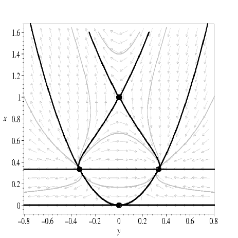
Figure 1: The phase space for the high energy regime system with $\epsilon=+1$ and $\alpha<-1$. The upper (lower) region corresponds to the case B1 (C1).

The phase space of the system is considered when $\alpha<-1$ and is shown in Fig. 1. The lowest horizontal line ($x=0$) is the separatrix for open models ($K=-1$) and will be referred to as the open Friedmann separatrix (OFS). The trajectories on the separatrix represent Milne models ($x=0$, $K=-1$ and $a(\eta)\propto\eta$) which are equivalent to a Minkowski space-time in a hyperbolic co-ordinate system. The second higher horizontal line ($x_{\Lambda}=-(\alpha+1)$) is the separatrix which is the dividing line between regions of phantom ($x<x_{\Lambda}$) and non-phantom/standard behavior($x>x_{\Lambda}$), we will call this the phantom separatrix (PS). The standard region corresponds to the case B1, while the phantom region corresponds to the case C1. In the phantom region the fluid violates the Null Energy Condition ($\rho+P<0$). This means the energy density is increasing (decreasing) in the future for an expanding (contracting) universe. In the standard case of the linear EoS in GR, this occurs when ${\it w}<-1$ and ultimately leads to a Type I singularity BLJM ; CKW . The parabola ($y^{2}=x/3$) represents the separatrix for flat Friedmann models ($K=0$), we will call this the flat Friedmann separatrix (FFS). The inner most thick curve is the separatrix for closed Friedmann models ($K=+1$) and will be called the closed Friedmann separatrix (CFS). The separatrix has the form:

$$y^{2}=\frac{x}{3}-\left[\frac{A(\alpha+1)x}{(\alpha+1)+\epsilon x}\right]^{\frac{2}{3(\alpha+1)}}.$$ (36)

The constant $A$ is fixed by ensuring that the saddle fixed point coincides with the fixed point representing the generalized Einstein static model ($E$). The constant is given in terms of the EoS parameters and has the form:

$$A=-\frac{2}{\epsilon(3\alpha+1)(\alpha+1)}\left(-\frac{\epsilon(3\alpha+1)}{9}\right)^{\frac{3(\alpha+1)}{2}}.$$ (37)

The Minkowski fixed point is located at the intersection of the OFS and FFS. The generalized flat de Sitter fixed points are located at the intersection of the PS and FFS. The generalized Einstein static fixed point is located on the CFS. The trajectories between the OFS and the PS ($0<x<x_{\Lambda}$) represent models which exhibit phantom behavior (the case C1). The open models in the phantom region are asymptotic to a Milne model in the past and to a generalized flat de Sitter model ($dS_{+}$) in the future. The closed models in the phantom region evolve from a contracting de Sitter phase, through a phantom phase to an expanding de Sitter phase (phantom bounce). It is interesting to note that unlike the standard GR case the phantom behavior does not result in a Type I singularity but asymptotically evolves to a expanding de Sitter phase. This is similar to the behavior seen in the phantom generalized Chaplygin gas case BLJM . The trajectories on the PS all represent generalized de Sitter models ($x^{\prime}=0$). The fixed points represent generalized flat de Sitter models ($K=0$). The open model on the PS represent generalized open de Sitter models ($K=-1$) in hyperbolic co-ordinates. The closed models on the PS evolve from a contracting phase to an expanding phase and represent generalized closed de Sitter models ($K=+1$). The Friedmann equation can be solved for such models to give:

$$\begin{array}[]{ll}a(\eta)=\sqrt{\frac{3}{x_{o}}}\cosh\left[\sqrt{\frac{x_{o}}{3}}(\eta-\eta_{o})\right]{}{}&\mbox{for $k=1$}\,,\\ \\ a(\eta)=\mbox{e}^{\sqrt{\frac{x_{o}}{3}}(\eta-\eta_{o})}&\mbox{for $k=0$}\,,\\ \\ a(\eta)=\sqrt{\frac{3}{x_{o}}}\sinh\left[\sqrt{\frac{x_{o}}{3}}(\eta-\eta_{o})\right]&\mbox{for $k=-1$}\,,\end{array}$$ (38)

The region above the PS represents models which evolve in a non-phantom/standard manner (the case B1). The trajectories in the expanding region ($y>0$) of the phase space are asymptotic to a Type III singularity in the past. The trajectories outside the FFS represent open models which evolve from a Type III singularity to a flat de Sitter phase, as do the trajectories on the FFS. The trajectories in between the CFS and the FFS evolve from a Type III singularity to a flat expanding de Sitter phase but may enter a phase of loitering. Loitering is characterized by the Hubble parameter dipping to a low value over a narrow red-shift range, followed by a rise again. In order to see this more clearly, we have plotted the normalized Hubble parameter ($y$) as a function of scale factor for three different trajectories in Fig. 2.

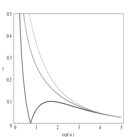
Figure 2: The normalized Hubble parameter, $y$ for models with differing curvature. Starting from the top we have open, flat and the closed models.

The top two curves represent the open and flat models, with the Hubble parameter dropping off quicker for the flat Friedmann model. The lower most curve is the Hubble parameter for the closed model. The plot shows that the closed model evolves to a loitering phase. Loitering cosmological models in standard cosmology were first found for closed FLRW models with a cosmological constant. More recently, brane-world models which loiter have been found  SS , these models are spatially flat but can behave dynamically like a standard FLRW closed model. The interesting point here is that the models mentioned above loiter without the need of a cosmological constant (due to the appearance of an effective cosmological constant), the topology is asymptotically closed in the past and flat in the future. The trajectories inside the CFS can have two distinct types of behavior corresponding to the central regions above and below the generalized Einstein static fixed point. Trajectories in the lower region represent closed models which evolve from a contracting de Sitter phase, bounce and then evolve to a expanding de Sitter phase. The trajectories in the upper region evolve from a Type III Singularity, expand to a maximum $a$ (minimum $x$) and then re-collapse to a Type III singularity (we will refer to such re-collapsing models as turn-around models).

III.3.2 The $-1<\alpha<-1/3$ sub-case

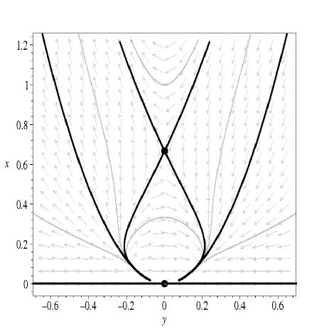
Figure 3: The phase space for the high energy regime system with $\epsilon=+1$ and $-1<\alpha<-1/3$. The entire region corresponds to the case A1.

The phase space for the system when $-1<\alpha<-1/3$ is shown in Fig. 3. The fixed points representing the flat generalized de Sitter models are no longer in the physical region ($x>0$) of the phase space. The open, flat and closed Friedmann separatrices (OFS, FFS and CFS) remains the same. The phantom separatrix (PS) is no longer present and all trajectories represent models with non-phantom/standard fluids (this corresponds to the case A1). The main difference is that the generic future attractor is now the Minkowski model. The trajectories between the OFS and FFS now evolve from a Type III singularity to a Minkowski model, as do the flat Friedmann models. The models between the FFS and CFS now evolve from a Type III singularity to a Minkowski with the possibility of entering a loitering phase (as before the model is asymptotically flat in the future). The trajectories inside the CFS and above the Einstein static fixed point still represent turn-around models. The trajectories inside the OFS and below the Einstein static model now represent standard bounce models, that is they evolve from a Minkowski model, contract to a finite size, bounce and then expand to a Minkowski model.

III.3.3 The $\alpha\geq-1/3$ sub-case

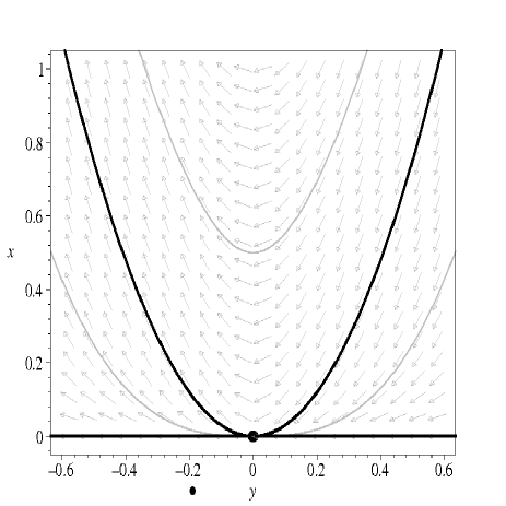
Figure 4: The phase space for the high energy regime system with $\epsilon=+1$ and $\alpha\geq-1/3$. The entire region corresponds to the case A1.

Next we consider the system when $\alpha\geq-1/3$, the phase space is shown in Fig. 4. The fixed point representing the Einstein static models is now located in the $x<0$ region of the phase space. The fluid in the entire physical region behaves in a non-phantom manner and corresponds to the case A1. The OFS and FFS remain the same and the CFS is no longer present. The trajectories between the OFS and FFS evolve from a Type III singularity to a Minkowski model. All trajectories above the FFS now represent turn-around models which start and terminate at a Type III singularity. The behavior of the models is qualitatively the same as that of the standard FLRW model with a linear EoS where ${\it w}=\alpha$, in the linear EoS case the Type III singularity is replaced by a standard “Big Bang”.

III.4 The $\epsilon=-1$ case

We now consider the system when we have a negative quadratic energy density term ($\epsilon=-1$) in the high energy regime EoS. The character of the fixed point M is still undefined. The fixed point representing the generalized Einstein static model is now a center. The fixed points representing the expanding/contracting flat de Sitter points now have saddle stability. As before, the trajectories or fixed points in the $y>0$ ($y<0$) region represent expanding models (contracting models), the black lines represent separatrix, grey lines represent example trajectories and fixed points are represented by black dots.

III.4.1 The $\alpha<-1$ sub-case

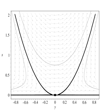
Figure 5: The phase space for the high energy regime system with $\epsilon=-1$ and $\alpha<-1$. The entire region corresponds to the case A2.

The phase space of the system when $\alpha<-1$ is shown in Fig. 5. The horizontal line ($x=0$) is still the open Friedman separatrix (OFS). The parabola is the flat Friedmann separatrix (FFS). The intersection of the OFS and FFS coincides with the Minkowski fixed point. All the trajectories in the physical region of the phase space exhibit phantom behavior (corresponding to the case A2), the energy density increases in an expanding model. The trajectories in the expanding (contracting) region in general evolve to a Type III singularity in the future (past). The trajectories between the OFS and the FFS are asymptotic to a Milne model in the past and are asymptotic to a Type III singularity in the future. The trajectories on the FFS start from a Minkowski model and enter a phase of super-inflationary expansion and evolve to a Type III singularity. Trajectories that start in a contracting phase during which the energy density decreases, reach a minimum $a$ (minimum $x$) and then expand where the energy density increases represent phantom bounce models. The trajectories above the FFS represent closed models which evolve through a phantom bounce, but start and terminate in a Type III singularity. The behavior of the models is qualitatively the same as that of the FLRW models with a phantom linear EoS (${\it w}<-1$) except that the Type III singularity is replaced by a Type I (“Big Rip”) singularity.

III.4.2 The $-1<\alpha<-1/3$ sub-case

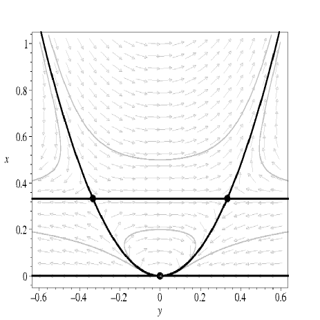
Figure 6: The phase space for the high energy regime system with $\epsilon=-1$ and $-1<\alpha<-1/3$. The upper (lower) region corresponds to the case B2 (C2).

The phase space for the system when $-1<\alpha<-1/3$ is shown in Fig. 6. The lowest horizontal line ($x=0$) is the OFS. The second higher horizontal line, $x_{\Lambda}=(\alpha+1)$ is the phantom separatrix (PS), this divides the state space into regions of phantom ($x>x_{\Lambda}$) and non-phantom/standard behavior ($x<x_{\Lambda}$). The phantom region corresponds to the case B2 and the standard region corresponds to the case C2. The flat de Sitter ($dS_{\pm}$) points are located at the intersection of the FFS and the PS. The open models in the standard matter region ($0<x<x_{\Lambda}$) are past asymptotic to open expanding de Sitter models in the past and evolve to Minkowski models in the future. The closed models in the region represent the standard bounce models, that is they evolve from a Minkowski model, contract to a minimum $a$ (maximum $x$) and then expand to a Minkowski model. The trajectories above the PS ($x>(\alpha+1)$) all exhibit phantom behavior. The open models in this region are past asymptotic to open de Sitter models in the past and evolve to a Type III singularity in the future. The closed models in the region all represent models which undergo a phantom bounce but start and terminate in a Type III singularity.

III.4.3 The $\alpha\geq-1/3$ sub-case

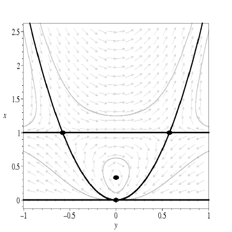
Figure 7: The phase space for the high energy regime system with $\epsilon=-1$ and $\alpha\geq-1/3$. The upper (lower) region corresponds to the case B2 (C2).

We now consider the system when $\alpha\geq-1/3$, the phase space is shown in Fig. 7. The OFS, FFS and the PS are all still present, the phantom regions still corresponds to the case B2 and the standard region to the case C2. The trajectories in the phantom region ($x>x_{\Lambda}$) behave in a similar manner to the previous case, as do the open models in the standard matter region ($0<x<x_{\Lambda}$). The main difference is in the region representing closed models ($K=1$) with non-phantom behavior. There is now a new fixed point which represents a generalized Einstein static model ($E$). The closed models in the region now represent oscillating models. This is represented by closed concentric loops centered on the Einstein static fixed point. These oscillating models also appear in the low energy system and will be discussed in more detail later.

IV Low energy regime Dynamics

IV.1 The dimensionless dynamical system

We now consider the system of equations for the low energy regime EoS, which can be simplified and expressed in terms of the following dimensionless variables:

$$x=\frac{\rho}{|P_{o}|}\;,~{}~{}y=\frac{H}{\sqrt{|P_{o}|}}\;,~{}~{}\eta=\sqrt{|P_{o}|}t\;.$$ (39)

The system of equations is then:

$$y^{2} = \frac{x}{3}-\frac{K}{|P_{o}|a^{2}},$$ (40)

$$y^{\prime} = -y^{2}-\frac{1}{6}\left(3\epsilon_{p}+(3\alpha+1)x\right),$$ (41)

$$x^{\prime} = -3y\left(\epsilon_{p}+(\alpha+1)x\right).$$ (42)

The discrete parameter $\epsilon_{p}$ denotes the sign of the pressure term, $\epsilon_{p}\in\{-1,1\}$. The primes denote differentiation with respect to the new $\eta$. The variables $x$ and $y$ are the new normalized energy density and Hubble parameter. As before only the positive energy density region of the phase space will be considered. The fixed points of the system and the existence conditions are given in Table 4. As before, by existence we mean the conditions on the parameters to insure $x\geq 0$ and $x,y\in\mathbb{R}$.

Table 4: Location and existence conditions of the fixed points of the low energy regime system.

Name	$x$	$y$	Existence
$E$	$-\frac{3\epsilon_{p}}{(3\alpha+1)}$	$0$	$\frac{\epsilon_{p}}{(3\alpha+1)}<0$
$dS_{+}$	$-\frac{\epsilon_{p}}{(\alpha+1)}$	$+\sqrt{\frac{-\epsilon_{p}}{3(\alpha+1)}}$	$\frac{\epsilon_{p}}{(\alpha+1)}<0$
$dS_{-}$	$-\frac{\epsilon_{p}}{(\alpha+1)}$	$-\sqrt{\frac{-\epsilon_{p}}{3(\alpha+1)}}$	$\frac{\epsilon_{p}}{(\alpha+1)}<0$

The Minkowski model ($x=y=0$) is no longer a fixed point of the system. The first fixed point (E) represents a generalized static Einstein model. This requires the overall effective equation of state to be that of inflationary matter and therefore only exists when $\epsilon_{p}/(3\alpha+1)<0$. The last two points represent generalized expanding and contracting flat de Sitter models. These points only exist if the fluid permits an effective cosmological constant point $\tilde{x}_{\Lambda}=\tilde{\rho}_{\Lambda}/{|P_{o}|}=-\epsilon_{p}/(\alpha+1)$, also $\tilde{x}_{\Lambda}\geq 0$ for the points to be in the physical region of the phase space. The eigenvalues of the equilibrium points are given in Table 5, while the linear stability character is given in Table 6.

Table 5: Eigenvalues of the fixed points of the low energy regime system.

Name	$\lambda_{1}$	$\lambda_{2}$
$E$	$\sqrt{-\epsilon_{p}}$	$-\sqrt{-\epsilon_{p}}$
$dS_{+}$	$\sqrt{\frac{-3(\alpha+1)}{\epsilon_{p}}}$	$-\frac{2}{\sqrt{-3\epsilon_{p}(\alpha+1)}}$
$dS_{-}$	$-\sqrt{\frac{-3(\alpha+1)}{\epsilon_{p}}}$	$\frac{2}{\sqrt{-3\epsilon_{p}(\alpha+1)}}$

Table 6: The linear stability of the fixed points for the low energy regime system.

Name	$\epsilon_{p}=+1$	$\epsilon_{p}=-1$
$E$	Center ($\alpha\neq-1/3$)	Saddle ($\alpha\neq-1/3$)
$dS_{+}$	Saddle ($\alpha<-1$)	Attractor ($\alpha>-1$)
$dS_{-}$	Saddle ($\alpha<-1$)	Repeller ($\alpha>-1$)

IV.2 The $\epsilon_{p}=+1$ case

We start by considering the system when we have a positive constant pressure term ($\epsilon_{p}=+1$) in the low energy regime EoS. The Minkowski ($x=y=0$) point is no longer present and the Einstein static solution has the stability character of a center. The fixed points representing the generalized expanding/contracting de Sitter points ($dS_{\pm}$) now have saddle stability. As before black lines represent separatrix, grey lines represent example trajectories and black dots represent fixed points of the system.

IV.2.1 The $\alpha<-1$ sub-case

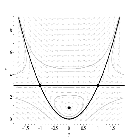
Figure 8: The phase space for the low energy regime system with $\epsilon_{p}=+1$ and $\alpha<-1$. The upper (lower) region corresponds to the case E1 (F1).

The phase space for the system when $\alpha<-1$ is shown in Fig. 8. The open Friedmann separatrix ($x=0$) is no longer present, and the $x=y=0$ point is no longer a fixed point of the system. The horizontal line ($\tilde{x}_{\Lambda}=-(\alpha+1)^{-1}$) is the phantom separatrix (PS), dividing the state space into regions with phantom ($x>\tilde{x}_{\Lambda}$) and standard ($x<\tilde{x}_{\Lambda}$) behavior. The phantom region corresponds to the case E1 and the standard region corresponds to the case F1. The parabola $y^{2}=x/3$ is the separatrix representing the flat Friedmann models (FFS), this divides the remaining trajectories into open and closed models. The intersection of the PS and FFS coincides with the fixed points of the generalized flat de Sitter models.

The trajectories in the upper region that start in a contracting phase (during which the energy density decreases), reach a minimum $a$ (minimum $x$) and then expand, representing phantom bounce models which terminate in a Type I singularity. The closed models in the phantom region ($x>\tilde{x}_{\Lambda}$) represent phantom bounce models which start and terminate in a Type I singularity . The open models in the phantom region are asymptotic to open de Sitter models in the past and evolve to a Type I singularity in the future. The trajectories below the PS ($x<\tilde{x}_{\Lambda}$) represent models which all behave in a standard manner (the F1 case). The open models in this region are all non-physical as they all evolve to the $x<0$ region of the phase space. The region corresponding to closed models (above the FFS) contain a fixed point which represents the generalized Einstein static (E) model. The region is filled by a infinite set of concentric closed loops centered on the Einstein static fixed point, the closed loops represent oscillating models. The Friedmann equation for such models is given by:

$$y^{2}=\frac{x}{3}-K\left[\frac{\epsilon_{p}+(\alpha+1)x}{B(\alpha+1)}\right]^{\frac{2}{3(\alpha+1)}}.$$ (43)

The constant $B$ is fixed by the location of the Einstein fixed point ($E$). The constant is given in terms of $\alpha$ and $\epsilon_{p}$:

$$B=\frac{-2\epsilon_{p}}{(\alpha+1)(3\alpha+1)}\left(\frac{3\alpha+1}{-\epsilon_{p}}\right)^{\frac{3(\alpha+1)}{2}}.$$ (44)

These oscillating models appear for $-\infty<\alpha<-1/3$ when $\epsilon_{p}=+1$ and are qualitatively similar to the oscillating models seen in the high energy case. The exact behavior of the variables for these models can be calculated by fixing the EoS parameter $\alpha$. The qualitative behavior remains the same for the models, however the maximum and minimum values of the variables change. In the case of $\alpha=-2/3$ the equations are greatly simplified, the scale factor oscillates such that:

$$a(\eta)=a_{o}\left(1+\sqrt{{1-K}}\sin(\eta_{o}-\eta)\right)$$ (45)

The maximum and minimum scale factor is then:

$$a_{max}=a_{o}(1+\sqrt{{1-K}})\;,~{}~{}a_{min}=a_{o}(1-\sqrt{{1-K}})\;.$$ (46)

The normalized hubble parameter ($y$) is:

$$y=y_{o}\frac{\sqrt{{1-K}}\cos(\eta_{o}-\eta)}{1+\sqrt{{1-K}}\sin(\eta_{o}-\eta)}.$$ (47)

The maximum and minimum $y$ is given by:

$$y_{max}=y_{o}\sqrt{\frac{1-K}{K}}\;,~{}~{}y_{min}=-y_{o}\sqrt{\frac{1-K}{K}}\;.$$ (48)

The normalized energy density ($x$) is given by:

$$x=x_{o}\left(\frac{1-\sqrt{{1-K}}\sin(\eta_{o}-\eta)}{1+\sqrt{{1-K}}\sin(\eta_{o}-\eta)}\right).$$ (49)

The maximum and minimum $x$ are:

$$x_{max}=x_{o}\left(\frac{1+\sqrt{{1-K}}}{1-\sqrt{{1-K}}}\right)\;,~{}~{}x_{min}=x_{o}\left(\frac{1-\sqrt{{1-K}}}{1+\sqrt{{1-K}}}\right)\;.$$ (50)

IV.2.2 The $-1<\alpha<-1/3$ sub-case

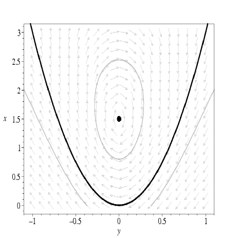
Figure 9: The phase space for the low energy regime system with $\epsilon_{p}=+1$ and $-1\leq\alpha<-1/3$. The entire region corresponds to the case D1.

We now consider the case when $-1<\alpha<-1/3$, the phase space is shown in Fig. 9. All trajectories in the physical region of the phase space exhibit standard behavior and correspond to the case D1. There is only one fixed point in the $x\geq 0$ region of the phase space, this point represents the generalized Einstein static model ($E$). The FFS represent models which evolve from a standard “Big Bang”, evolve to a Minkowski model and then to a standard “Big Crunch” (turn around model). The open models (below the FFS) are non-physical as the evolve into the $x<0$ region. The trajectories above the separatrix represent closed models ($K>0$) which oscillate indefinitely between a maximum and minimum $a$ (minimum and maximum $x$), as seen in the previous case.

IV.2.3 The $-1/3\leq\alpha$ sub-case

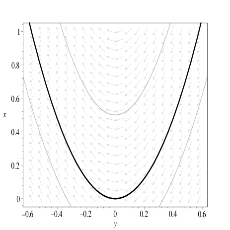
Figure 10: The phase space for the low energy regime system with $\epsilon_{p}=+1$ and $-1/3\leq\alpha$. The entire region corresponds to the case D1.

The phase space for the system when $-1/3\leq\alpha$ is shown in Fig. 10. As in the previous sub-case the fluid behaves in a standard manner and corresponds to the case D1. There are no fixed points in the physical region of the phase space. The parabola is the FFS and represents flat model which evolve from a “Big Bang”, approach a Minkowski model and then re-collapse (turn-around models) to a “Big Crunch”. The open models (below the FFS) are all non-physical as they evolve to the negative energy density region ($x<0$) of the phase space. The closed models evolve from a “Big Bang”, reach a maximum $a$ (minimum $x$) and re-collapse to a “Big Crunch”.

IV.3 The $\epsilon_{p}=-1$ case

We now consider the system when we have a negative constant pressure term ($\epsilon_{p}=-1$) in the low energy regime EoS. As before,the Minkowski ($x=y=0$) point is no longer a fixed point of the system and the OFS is not present. The fixed point representing the generalized Einstein static model ($E$) has the stability character of a saddle. The fixed points representing the generalized expanding (contracting) flat de Sitter points now have attractor (repeller) stability.

IV.3.1 The $\alpha<-1$ sub-case

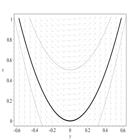
Figure 11: The phase space for the low energy regime system with $\epsilon_{p}=-1$ and $\alpha<-1$. The entire region corresponds to the case D2.

The phase space for the low energy system when $\alpha<-1$ is shown in Fig. 11. All the trajectories in the $x>0$ region of the phase space now exhibit phantom behavior and correspond to the case D2. The open models are all non-physical as they all evolve from the negative energy density region of the phase space. The flat and closed models represent phantom bounce models which start and end in a Type I singularity. They evolve from a Type I singularity, contract, bounce at a minimum $a$ (minimum $x$) and expand to a Type I singularity.

IV.3.2 The $-1<\alpha<-1/3$ sub-case

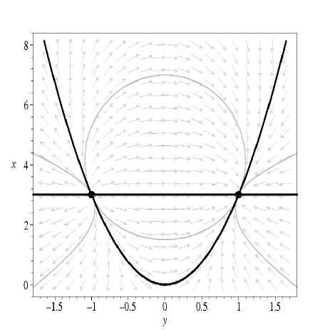
Figure 12: The phase space for the low energy regime system with $\epsilon_{p}=-1$ and $-1\leq\alpha<-1/3$. The upper (lower) region corresponds to the case E2 (F2).

The phase space for the system when $-1<\alpha<-1/3$ is shown in Fig. 12. The horizontal line, $\tilde{x}_{\Lambda}=(\alpha+1)^{-1}$ is the phantom separatrix (PS), dividing the state space into regions with phantom ($x<\tilde{x}_{\Lambda}$) and standard behavior ($x>\tilde{x}_{\Lambda}$). The standard region corresponds to the case E2 and the phantom region corresponds to the case F2. The intersection of the PS and FFS coincides with the fixed points of the generalized flat de Sitter models ($dS_{\pm}$). The flat expanding (contracting) de Sitter model is the generic future attractor (repeller). The open models in the standard matter region ($x>\tilde{x}_{\Lambda}$) evolve from a standard “Big Bang” to a flat expanding de Sitter phase. The closed models in this region evolve from a contracting flat de Sitter phase, reach a minimum $a$ (maximum $x$), bounce and then evolve to expanding flat de Sitter phase. These models represent standard bounce models with asymptotic de Sitter behavior. The open models in the phantom region ($x<\tilde{x}_{\Lambda}$) are all non-physical. The flat and closed models in this region represent models exhibiting phantom bounce behavior which avoid the “Big Rip” and instead evolve to an expanding flat de Sitter phase.

IV.3.3 The $-1/3\leq\alpha$ sub-case

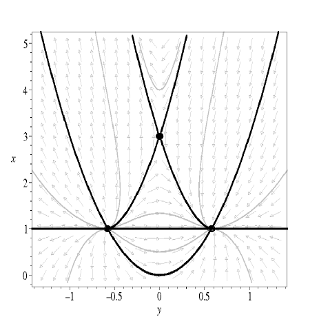
Figure 13: The phase space for the low energy regime system with $\epsilon_{p}=-1$ and $-1/3\leq\alpha$. The upper (lower) region corresponds to the case E2 (F2).

We now consider the system in the parameter range $-1/3\leq\alpha$, the phase space is shown in Fig. 13. The PS ($\tilde{x}_{\Lambda}=(\alpha+1)^{-1}$), FFS ($y^{2}=x/3$) and generalized flat de Sitter points ($dS_{\pm}$) still remain. The flat expanding (contracting) de Sitter model is the generic future attractor (repeller). The inner most black curve is the closed Friedmann separatrix (CFS) and coincides with the generalized Einstein static fixed point ($E$), which has saddle stability. The CFS is given by:

$$y^{2}=\frac{x}{3}-D\left[\frac{(\alpha+1)x-1}{2}\right]^{\frac{2}{3(\alpha+1)}}.$$ (51)

The constant $D$ is a constant of integration and can be fixed by the location of the fixed point $E$. The constant is given in terms of $\alpha$ and has the form:

$$D=\left({3\alpha+1}\right)^{-\frac{(3\alpha+1)}{3(\alpha+1)}}.$$ (52)

The region below the PS ($x<\tilde{x}_{\Lambda}$) remains qualitatively the same. The open models in the standard matter region ($x>\tilde{x}_{\Lambda}$) all evolve from a “Big Bang” to a expanding flat de Sitter phase. The trajectories between the FFS and the CFS also evolve from a “Big Bang” to a generalized expanding flat de Sitter model with the possibility of entering a loitering phase. The models inside the CFS can behave in one of two ways. The trajectories above the generalized Einstein static point represent turn-around models which evolve from a “Big Bang”, reach a maximum $a$ (minimum $x$) and then re-collapse to a “Big Crunch”. The trajectories below evolve from a contracting de Sitter phase to an expanding de Sitter phase and represent bounce models.

V The Full system

Table 7: The locations of the fixed points of the full system. The existence conditions are also given, that is $x,y,\in\mathbb{R}$ and $x\geq 0$. To simplify the expressions special values of $\nu$ are used which can be expressed in terms of $\alpha$, these values are $\nu_{1}=\frac{(3\alpha+1)^{2}}{36}$ and $\nu_{2}=\frac{(\alpha+1)^{2}}{4}$.

Name	$x$	$y$	Existence ($\epsilon=+1$)	Existence ($\epsilon=-1$)
$M$	$0$	$0$	$\nu=0$	$\nu=0$
$E_{1}$	$-\frac{(3\alpha+1)}{6\epsilon}+\frac{\sqrt{(3\alpha+1)^{2}-36\epsilon\nu}}{6\epsilon}$	$0$	$\nu\leq\nu_{1}$, $\alpha<-1/3$	$-\nu_{1}<\nu<0$, $\alpha>-1/3$
			$\nu<0$, $\alpha>-1/3$
$E_{2}$	$-\frac{(3\alpha+1)}{6\epsilon}-\frac{\sqrt{(3\alpha+1)^{2}-36\epsilon\nu}}{6\epsilon}$	$0$	$0<\nu<\nu_{1}$, $\alpha<-1/3$	$\nu>0$ , $\alpha<-1/3$
				$\nu\geq-\nu_{1}$, $\alpha>-1/3$
$dS_{1,\pm}$	$-\frac{(\alpha+1)}{2\epsilon}+\frac{\sqrt{(\alpha+1)^{2}-4\epsilon\nu}}{2\epsilon}$	$\pm\left(-\frac{(\alpha+1)}{6\epsilon}+\frac{\sqrt{(\alpha+1)^{2}-4\epsilon\nu}}{6\epsilon}\right)^{\frac{1}{2}}$	$\nu\leq\nu_{2}$, $\alpha<-1$	$-\nu_{2}<\nu<0$, $\alpha>-1$
			$\nu<0$, $\alpha>-1$
$dS_{2,\pm}$	$-\frac{(\alpha+1)}{2\epsilon}-\frac{\sqrt{(\alpha+1)^{2}-4\epsilon\nu}}{2\epsilon}$	$\pm\left(-\frac{(\alpha+1)}{6\epsilon}-\frac{\sqrt{(\alpha+1)^{2}-4\epsilon\nu}}{6\epsilon}\right)^{\frac{1}{2}}$	$0<\nu<\nu_{2}$, $\alpha<-1$	$\nu>0$, $\alpha<-1$
				$-\nu_{2}\leq\nu$, $\alpha>-1$

V.1 The dimensionless dynamical system

We now consider the system of equations with the full quadratic EoS, this can be simplified in a similar fashion to the previous case by introducing a new set variables:

$$x=\frac{\rho}{|\rho_{c}|}\;,~{}~{}y=\frac{H}{\sqrt{|\rho_{c}|}}\;,~{}~{}\eta=\sqrt{|\rho_{c}|}t\;,~{}~{}\nu=\frac{P_{o}}{\sqrt{|\rho_{c}|}}\;.$$ (53)

The system of equations then become:

$$y^{2} = \frac{x}{3}-\frac{K}{|\rho_{c}|a^{2}},$$ (54)

$$y^{\prime} = -y^{2}-\frac{1}{6}\left(3\nu+(3\alpha+1)x+3\epsilon x^{2}\right),$$ (55)

$$x^{\prime} = -3y\left(\nu+(\alpha+1)x+\epsilon x^{2}\right).$$ (56)

The parameter $\epsilon$ denotes the sign of the quadratic term, $\epsilon\in\{-1,1\}$. The parameter $\nu$ is the normalized constant pressure term. The primes denote differentiation with respect to the new normalized time variable $\eta$ and only the physical region of the phase space is considered ($x\geq 0$). The fixed points and their existence conditions are given in Table 7. The phase space undergo’s a topological change for special values of the $\nu$ parameter, these values can be expressed in terms of $\alpha$ and are:

$$\nu_{1}=\frac{(3\alpha+1)^{2}}{36},\qquad\nu_{2}=\frac{(\alpha+1)^{2}}{4}.$$ (57)

Table 8: The linear stability character of the fixed points for the full system. The stability character is only valid for choices of parameters which are consistent with the existence conditions and constraints given below.

Name	$\epsilon=\pm 1$	Exceptions
$M$	Undefined	-
$E_{1}$	Saddle	$36\epsilon\nu\neq(3\alpha+1)^{2}$
$E_{2}$	Center	$36\epsilon\nu\neq(3\alpha+1)^{2}$
$\,dS_{1,+}\,$	Attractor	$4\epsilon\nu\neq(\alpha+1)^{2}$
$\,dS_{1,-}\,$	Repeller	$4\epsilon\nu\neq(\alpha+1)^{2}$
$\,dS_{2,+}\,$	Saddle	$4\epsilon\nu\neq(\alpha+1)^{2}$
$\,dS_{2,-}\,$	Saddle	$4\epsilon\nu\neq(\alpha+1)^{2}$

Table 9: The Eigenvalues derived from the linear stability analysis of the fixed points for the full system. In order to simplify the form of the eigenvalues we introduce the following variables, $\gamma_{1}=(3\alpha+1)$, $\gamma_{2}=(\alpha+1)$ and $\delta=\sqrt{(\alpha+1)^{2}-4\epsilon\nu}$. These eigenvalues are only valid for the choice of parameters consistent with the existence conditions.

Name	$\lambda_{1}$	$\lambda_{2}$
$M$	$0$	$0$
$E_{1}$	$+\left(\frac{\gamma_{1}^{2}-\gamma_{1}\sqrt{\gamma_{1}^{2}-36\epsilon\nu}-36\epsilon\nu}{18\epsilon}\right)^{\frac{1}{2}}$	$-\left(\frac{\gamma_{1}^{2}-\gamma_{1}\sqrt{\gamma_{1}^{2}-36\epsilon\nu}-36\epsilon\nu}{18\epsilon}\right)^{\frac{1}{2}}$
$E_{2}$	$+\left(\frac{\gamma_{1}^{2}+\gamma_{1}\sqrt{\gamma_{1}^{2}-36\epsilon\nu}-36\epsilon\nu}{18\epsilon}\right)^{\frac{1}{2}}$	$-\left(\frac{\gamma_{1}^{2}+\gamma_{1}\sqrt{\gamma_{1}^{2}-36\epsilon\nu}-36\epsilon\nu}{18\epsilon}\right)^{\frac{1}{2}}$
$dS_{1,\pm}$	$\mp\sqrt{\frac{\delta-\gamma_{2}}{6\epsilon}}\left(1+\frac{3\delta}{2}\right)+\left(\frac{{6\delta^{2}}(3\delta-3\gamma_{2}-4)+8(\gamma_{2}(3\delta-1)+\delta)}{48\epsilon}\right)^{\frac{1}{2}}$	$\mp\sqrt{\frac{\delta-\gamma_{2}}{6\epsilon}}\left(1+\frac{3\delta}{2}\right)-\left(\frac{{6\delta^{2}}(3\delta-3\gamma_{2}-4)+8(\gamma_{2}(3\delta-1)+\delta)}{48\epsilon}\right)^{\frac{1}{2}}$
$dS_{2,\pm}$	$\pm\sqrt{\frac{-(\delta+\gamma_{2})}{6\epsilon}}\left(\frac{3\delta}{2}-1\right)+\left(-\frac{{6\delta^{2}}(3\delta+3\gamma_{2}+4)+8(\gamma_{2}(3\delta+1)+\delta)}{48\epsilon}\right)^{\frac{1}{2}}$	$\pm\sqrt{\frac{-(\delta+\gamma_{2})}{6\epsilon}}\left(\frac{3\delta}{2}-1\right)-\left(-\frac{{6\delta^{2}}(3\delta+3\gamma_{2}+4)+8(\gamma_{2}(3\delta+1)+\delta)}{48\epsilon}\right)^{\frac{1}{2}}$

As in the previous case, by existence we mean $x\geq 0$ and $x,y\in\mathbb{R}$. The general eigenvalues derived from the linear stability analysis are given in Table 9. The linear stability character of the fixed points is given in Table 8.

The system has six fixed points and the sign of $\epsilon$ no longer effects the linear stability character of the fixed point (but changes it’s position in the $x-y$ plane). The first fixed point $M$ represents a Minkowski model and is only present if $\nu=0$, the linear stability character is undefined. The second fixed point $E_{1}$ represents an Einstein static model and has the linear stability character of a saddle. The third fixed point $E_{2}$ represents an Einstein static model with the linear stability character of a center. In general, this fixed point is surrounded by a set of closed concentric loops representing oscillating models. The next pair of fixed points $dS_{1,\pm}$ represents a set of generalized flat de Sitter models, the expanding (contracting) model has attractor (repeller) stability. The next pair of fixed points $dS_{2,\pm}$ also represents a set of generalized flat de Sitter models, but now they have saddle stability. The separatrix for open Friedmann models (OFS) is only present if $\nu=0$. The parabola $y^{2}=x/3$ (FFS) still separates the open and closed models. The separatrix for the closed Friedmann models (CFS) is present for a narrow range of the parameters and always coincides with the fixed points representing the generalized Einstein static model, $E_{1}$. The fluid permits two possible effective cosmological constants points, they are given by:

$$x_{\Lambda,1} = \frac{\rho_{\Lambda,1}}{|\rho_{c}|}=-\frac{(\alpha+1)}{2\epsilon}+\frac{\sqrt{\delta}}{2\epsilon},$$ (58)

$$x_{\Lambda,2} = \frac{\rho_{\Lambda,2}}{|\rho_{c}|}=-\frac{(\alpha+1)}{2\epsilon}-\frac{\sqrt{\delta}}{2\epsilon}.$$ (59)

Where $\delta=(\alpha+1)^{2}-4\epsilon\nu$. There is also a separatrix associated with each of the effective cosmological points, which divide the regions of phantom and non-phantom behavior. The separatrices will be referred to as the phantom separatrix ($PS_{i}$ which corresponds to the line $x=x_{\Lambda,i}$), with the appropriate subscript. For special choices of parameters the separatrices coincide. The discussion of the system will be split into the two categories, $\epsilon=+1$ and $\epsilon=-1$.

V.2 The $\epsilon=+1$ case

We first consider the system when we have a positive quadratic energy density term ($\epsilon=+1$). The dynamical system can be further sub-divided into sub-cases with different values of the parameters $\alpha$ and $\nu$. The various subcases have been highlighted in Table 10.

Table 10: The various sub-cases of the full system when $\epsilon=+1$. The figure numbers given in bold, indicate the choice of variables for which the state space is qualitatively different to previously discussed cases.

	$\alpha<-1$	$-1\leq\alpha<-1/3$	$-1/3\leq\alpha$
$\nu>\nu_{1}$	FIG.10	FIG.10	FIG.10
$\nu=\nu_{1}$	FIG.14	FIG.14	FIG.10
$\nu_{2}<\nu<\nu_{1}$	FIG.15	FIG.15	FIG.10
$\nu=\nu_{2}$	FIG.16	FIG.15	FIG.10
$0<\nu<\nu_{2}$	FIG.17	FIG.15	FIG.10
$\nu=0$	FIG.1	FIG.3	FIG.4
$\nu<0$	FIG.13	FIG.13	FIG.13

The majority of sub-cases result in a phase space diagram which is qualitatively similar to cases discussed in previous sections. That is the qualitative behavior of trajectories is the same even though the functional form of $\rho(a)$ is different. The figure numbers not in bold (standard text) indicate choices of variable for which the phase space is qualitatively similar to a previous case, with the following differences:

• The regions which corresponded to different types of behavior of the fluid now change (replaced by new $\rho(a)$ behavior):

  • The case D1 $\to$ G1,

  • The case E2 $\to$ I3,

  • The case F2 $\to$ I2,

• The Type I singularities are now replaced by Type III singularities.

There is a narrow range of the parameters for which the state space is qualitatively different. The figure numbers given in bold in Table 10, indicate the choice of variables for which the state space is qualitatively different to previously discussed cases. We will now discuss the four sub-cases which are different to those discussed in previous sections.

V.2.1 The $\alpha<-1$, $\nu=\nu_{1}$ sub-case

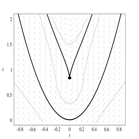
Figure 14: The phase space for the full system with $\epsilon=+1$, $\alpha<-1$ and $\nu=\nu_{1}$ (additionally when $\alpha<-1/3$ and $\nu=\nu_{1}$). The entire region corresponds to the case G1.

The phase space of the system when $\alpha<-1$ and $\nu=\nu_{1}$ is shown in Fig. 14. As before the black lines represent separatrix, grey lines represent example trajectories and fixed points are represented by black dots. The fluid behaves in a standard manner and corresponds to the case G1. This choice of parameters results in the two Einstein points ($E_{i}$) coinciding. The resulting fixed point is highly non-linear and cannot be classified into the standard linear stability categories as in previous cases. The fixed point coincides with the CFS and the parabola is the FFS. The open models are all non-physical as they evolve to the $x<0$ region of the phase space. The models between the FFS and the CFS represent turn-around models which evolve from a Type III singularity, evolve to a maximum $a$ (minimum $x$) and then re-collapse. The trajectories above the CFS also represent similar turn-around models.

V.2.2 The $\alpha<-1$, $\nu_{2}<\nu<\nu_{1}$ sub-case

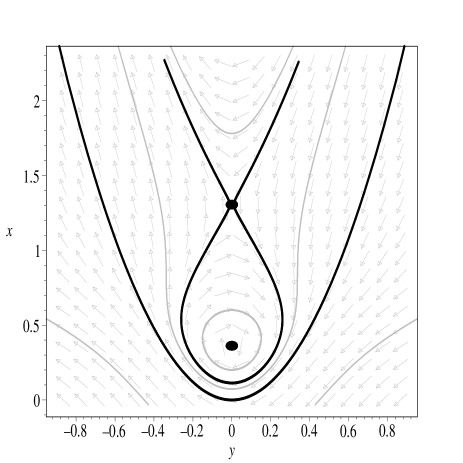
Figure 15: The phase space for the full system with $\epsilon=+1$, $\alpha<-1$ and $\nu_{2}<\nu<\nu_{1}$ (additionally when $-1<\alpha<-1/3$ and $0<\nu<\nu_{1}$). The entire region corresponds to the case G1.

The phase space of the system when $\alpha<-1$ and $\nu_{2}<\nu<\nu_{1}$ is shown in Fig. 15. The fluid behaves in a standard manner and corresponds to the case G1. The Einstein fixed point of the previous case splits into two individual Einstein fixed points ($E_{i}$) via bifurcation. The first Einstein fixed point ($E_{1}$) coincides with the CFS, while the second Einstein fixed point ($E_{2}$) is located inside the lower region enclosed by the CFS. Only the trajectories above the FFS differ from the previous case. The trajectories between the CFS and FFS still represent turn-around models which evolve from a Type III singularity but may now enter a loitering phase. The trajectories inside the CFS and above the Einstein fixed point ($E_{1}$), evolve from a Type III singularity, reach a maximum $a$ and then re-collapse to a Type III singularity. The trajectories below $E_{1}$ represent closed oscillating models, the closed loops are centered on the second Einstein fixed point ($E_{2}$).

V.2.3 The $\alpha<-1$, $\nu=\nu_{2}$ sub-case

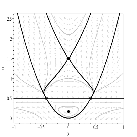
Figure 16: The phase space for the full system with $\epsilon=+1$, $\alpha<-1$ and $\nu=\nu_{2}$. The upper (lower) region corresponds to the case H2 (H1).

The phase space of the system when $\alpha<-1$ and $\nu=\nu_{2}$ is shown in Fig. 16. The fluid behaves in a standard manner in both regions and the upper (lower) region corresponds to the case H2 (H1). This choice of parameters results in the two sets of generalized de Sitter points ($dS_{i,\pm}$) coinciding. The fixed points coincide with $PS_{i}$ ($x=x_{\Lambda,i}$) and the FFS. The resulting fixed points are highly non-linear, the points have shunt stability along the FFS direction and the generalized expanding (contracting) de Sitter point has attractor (repeller) stability along the $PS_{i}$ direction. The two Einstein points ($E_{i}$) and the CFS are still present. In the $x<x_{\Lambda,i}$ region, the open models are all non-physical as they evolve to the $x<0$ region and the closed models represent oscillating models which are centered on the Einstein point ($E_{2}$) with center linear stability. In the $x>x_{\Lambda,i}$ region, the open models are asymptotic to a Type III singularity in the past and a expanding flat de Sitter phase ($dS_{i,+}$) in the future. The trajectories between the FFS and the CFS evolve from a Type III singularity to $dS_{i,+}$ with the possibility of entering a loitering phase. The models inside the CFS and above the $E_{1}$ point represent turn-around models which asymptotically approach a Type III singularity. The closed models inside the CFS and below the $E_{2}$ point are asymptotic to a contracting de Sitter model phase ($dS_{i,-}$) in the past and a expanding de Sitter phase ($dS_{i,+}$) in the future. The generic attractor in the $x>x_{\Lambda,i}$ region is the $dS_{i,+}$ fixed point.

V.2.4 The $\alpha<-1$, $0<\nu<\nu_{2}$ sub-case

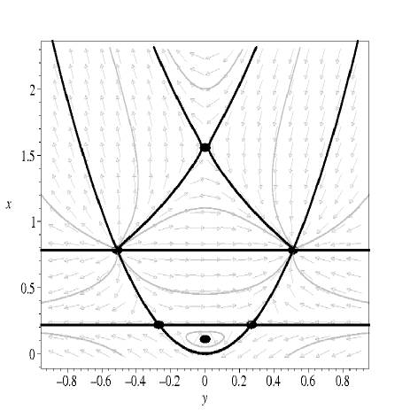
Figure 17: The phase space for the full system with $\epsilon=+1$, $\alpha<-1$ and $0<\nu<\nu_{2}$. The upper, middle and lower regions correspond to the cases I3, I2 and I1 respectively.

The phase space of the system when $\alpha<-1$ and $0<\nu<\nu_{2}$ is shown in Fig. 17. The upper (lower) horizontal line is the $PS_{1}$ ($PS_{2}$). The region above $PS_{1}$ corresponds to the case I3 and is qualitatively similar to the H2 region in the previous sub-case. The region below $PS_{2}$ corresponds to the case I1 and is qualitatively similar to the H1 region in the previous sub-case. The set of generalized flat de Sitter fixed points ($dS_{i,\pm}$) of the previous case split into two sets of generalized flat de Sitter fixed points via bifurcation. The upper (lower) set of generalized de Sitter points, $dS_{1,\pm}$ ($dS_{2,\pm}$) have attractor/repeller (saddle) stability. The region between $PS_{1}$ and $PS_{2}$ corresponds to the case I2 and the fluid behaves in a phantom manner. The open models in this region are asymptotic to open de Sitter models in the past and flat de Sitter models in the future. The closed models in the phantom region represent phantom bounce models which asymptotically approach a expanding (contracting) de Sitter phases in the future (past).

V.3 The $\epsilon=-1$ case

We now consider the system when we have a negative quadratic energy density term ($\epsilon=-1$). As before the system can be sub-divided into various sub-cases with different values of parameters of $\alpha$ and $\nu$. The various sub-cases have been highlighted in Table 11

Table 11: The various sub-cases of the $\epsilon=-1$ full system. The figure numbers given in bold, indicate the choice of variables for which the phase space is qualitatively different to previous cases.

	$\alpha<-1$	$-1\leq\alpha<-1/3$	$-1/3\leq\alpha$
$\nu>0$	FIG.8	FIG.8	FIG.8
$\nu=0$	FIG.5	FIG.6	FIG.7
$-\nu_{1}<\nu<0$	FIG.11	FIG.20	FIG.18
$\nu=-\nu_{1}$	FIG.11	FIG.20	FIG.19
$-\nu_{2}<\nu<-\nu_{1}$	FIG.11	FIG.20	FIG.20
$\nu=-\nu_{2}$	FIG.11	FIG.21	FIG.21
$\nu<-\nu_{2}$	FIG.11	FIG.11	FIG.11

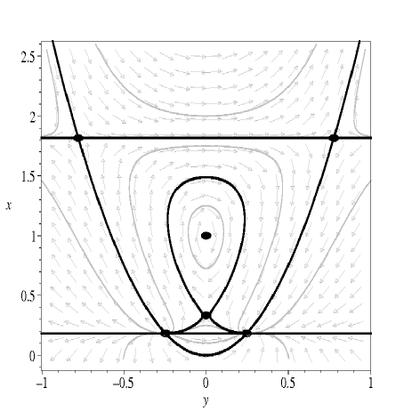
Figure 18: The phase space for the full system with $\epsilon=-1$, $\alpha>-1/3$ and $-\nu_{1}<\nu<0$. The upper, middle and lower regions correspond to the cases I6, I5 and I4 respectively.

As before, the figure numbers not in bold (standard text) indicate choices of variable for which the phase space is qualitatively similar to a previous case, with the following differences:

• The regions which corresponded to different types of behavior of the fluid now change (replaced by new form of $\rho(a)$):

  • The case D2 $\to$ G2,

  • The case E1 $\to$ I6,

  • The case F1 $\to$ I5,

• The Type I singularities are now replaced by Type III singularities.

There are choices of parameters for which the phase space is different (figure numbers in bold in Table 11) and these four sub-cases will be discussed in the following sections.

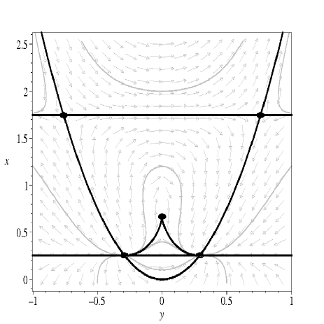
Figure 19: The phase space for the full system with $\epsilon=-1$, $\alpha>-1/3$ and $\nu=-\nu_{1}$. The upper, middle and lower regions correspond to the cases I6, I5 and I4 respectively.

V.3.1 The $\alpha>-1/3$, $-\nu_{1}<\nu<0$ sub-case

The phase space of the system when $\alpha>-1/3$ and $-\nu_{1}<\nu<0$ is shown in Fig. 18. The upper (lower) horizontal line at $x=x_{\Lambda,2}$ ($x=x_{\Lambda,1}$) is the $PS_{2}$ ($PS_{1}$) (they have swapped position with respect to the $\epsilon=+1$ case). The region above $PS_{2}$ corresponds to the case I6, the region below $PS_{1}$ corresponds to the case I4 and the fluid behaves in a phantom manner in both regions. The region between $PS_{1}$ and $PS_{2}$ corresponds to the case I5 and the fluid behaves in a standard manner. The lower set of generalized de Sitter points ($dS_{1,\pm}$ - at the intersection of $PS_{1}$ and FFS) have attractor/repeller stability, while the upper set ($dS_{2,\pm}$ - at the intersection of $PS_{2}$ and FFS) have saddle stability. The CFS is located in between $PS_{1}$ and $PS_{2}$ and coincides with the Einstein point ($E_{1}$). The open models in the $x<x_{\Lambda,1}$ region (the case I4) are all non-physical as they evolve from the $x<0$ region of the phase space. The closed models in this region represent phantom bounce models which evolve from a contracting de Sitter phase ($dS_{1,-}$) to a expanding de Sitter phase ($dS_{1,+}$). The open models in the standard region ($x_{\Lambda,1}<x<x_{\Lambda,2}$ corresponding to the case I5 ) are asymptotic to a generalized open de Sitter model in the past and generalized flat de Sitter model in the future (the future attractor has lower $x$ and $y$). The models between the CFS and the FFS in this region represent bounce models which evolve from a contracting de Sitter phase to a expanding de Sitter phase with the possibility of entering a loitering phase. The models enclosed by the CFS can be split into two groups. The models above the fixed point, $E_{1}$ represent oscillating models, the closed loops are centered on the fixed point $E_{2}$. The models below the fixed point, $E_{1}$ represent bounce models which evolve from $dS_{1,-}$ to $dS_{1,+}$. In the $x>x_{\Lambda,2}$ region (the case I6) the open models are asymptotic to generalized open de Sitter models in the past and a Type III singularity in the future. The closed models in this region represent phantom bounce models which evolve from a Type III singularity, reach a minimum $a$ (minimum $x$) and then evolve to a Type III singularity. The generalized expanding flat de Sitter model, $dS_{1,+}$ (Type III singularity) is the generic future attractor in the region $x<x_{\Lambda,2}$ ($x>x_{\Lambda,2}$). The trajectories in the regions, $x<x_{\Lambda,1}$ and $x>x_{\Lambda,2}$ remain qualitatively similar in the following two cases (Fig.19, 20).

V.3.2 The $\alpha>-1/3$, $\nu=-\nu_{1}$ sub-case

The phase space of the system when $\alpha>-1/3$ and $\nu=-\nu_{1}$ is shown in Fig. 19. The phase space is equivalent to the previous sub-case, except for the region $x_{\Lambda,1}<x<x_{\Lambda,2}$ (the case I5). The open models in this region are still asymptotic to generalized open (flat) de Sitter models in the past (future). The behavior of the closed models has now changed, there are no longer trajectories representing oscillating models. The two generalized Einstein fixed points ($E_{i}$) have now coalesced to form one fixed point via bifurcation. The closed models above $E_{i}$ represent bounce models which evolve from $dS_{1,-}$ to $dS_{1,+}$, with the possibility of entering a loitering phase. The closed models below $E_{i}$ represent bounce models which evolve from $dS_{1,-}$ to $dS_{1,+}$ without entering a loitering phase.

V.3.3 The $\alpha>-1/3$, $-\nu_{2}<\nu<-\nu_{1}$ sub-case

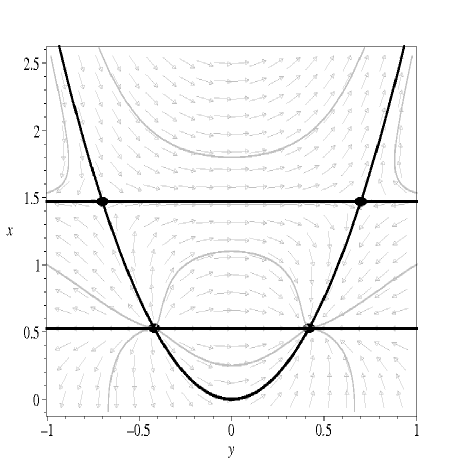
Figure 20: The phase space for the full system with $\epsilon=-1$, $\alpha>-1/3$ and $-\nu_{2}<\nu<-\nu_{1}$ (additionally when $-1<\alpha<-1/3$ and $-\nu_{2}<\nu<0$). The upper, middle and lower regions correspond to the cases I6, I5 and I4 respectively.

The phase space of the system when $\alpha>-1/3$ and $-\nu_{2}<\nu<-\nu_{1}$ is shown in Fig. 20. The phase space is qualitatively similar to the previous sub-cases except for the $x_{\Lambda,1}<x<x_{\Lambda,2}$ region. There are no longer any fixed points representing generalized Einstein static models and the CFS is no longer present. The open models in the region behave as in previous sub-cases. The closed models in the region represent bounce model, which evolve to a expanding (collapsing) de Sitter phase in the future (past) without the possibility of entering a loitering phase.

V.3.4 The $\alpha>-1/3$, $\nu=-\nu_{2}$ sub-case

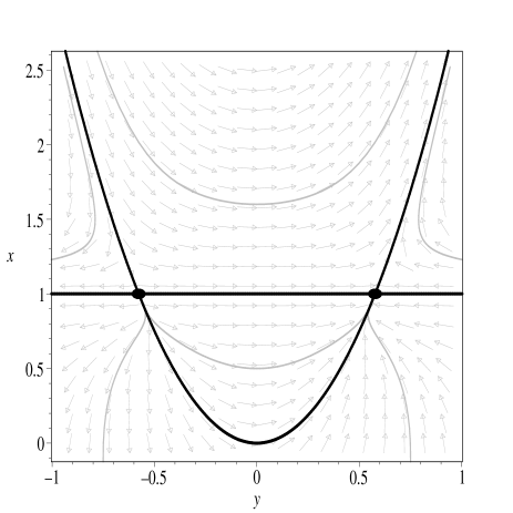
Figure 21: The phase space for the full system with $\epsilon=-1$, $\alpha>-1/3$ and $\nu=-\nu_{2}$ (additionally when $-1<\alpha<-1/3$ and $\nu=-\nu_{2}$). The upper (lower) region corresponds to the case H4 (H3).

The next case is the phase space of the system when $\alpha>-1/3$ and $\nu=-\nu_{2}$ and is shown in Fig. 21. The fluid behaves in a phantom manner in both regions and the upper (lower) region corresponds to the case H4 (H3). The two sets of generalized de Sitter points ($dS_{i,\pm}$) have now coalesced into a single set of generalized de Sitter points ($dS_{\pm}$) which are located at the intersection of the FFS and the $PS_{i}$ which have also coalesced to form a single separatrix ($x_{\Lambda,1}=x_{\Lambda,2}$). The resulting fixed points are highly non-linear, the points have shunt stability along the FFS direction and the generalized expanding (contracting) de Sitter point has attractor (repeller) stability along the $PS_{i}$ direction. The Type III singularity is the generic attractor in the upper region ($x>x_{\Lambda,i}$) and the $dS_{i,+}$ is the generic attractor in the lower region ($x<x_{\Lambda,i}$).

VI Discussion and Conclusions

In this paper we have systematically studied the dynamics of homogeneous and isotropic cosmological models containing a fluid with a quadratic EoS. This has it’s own specific interest (see Section I for a variety of motivations) and serves as a simple example of more general EoS’s. It can also be taken to represent the truncated Taylor expansion of any barotropic EoS, and as such it serves (with the right choice of parameters) as a useful phenomenological model for dark energy, or even UDM. Indeed, we have shown the dynamics to be very different and much richer than the standard linear EoS case, finding that an almost generic feature of the evolution is the existence of an accelerated phase, most often asymptotically de Sitter, thanks to the appearance of an effective cosmological constant. Of course to properly build physical cosmological models would require to consider the quadratic EoS for dark energy or UDM together with standard matter and radiation. Our analysis was aimed instead to derive and classify the large variety of different dynamical effects that the quadratic EoS fluid has when is the dominant component. In this respect, it should be noticed that a positive quadratic term in the EoS allows, in presence of another fluid such as radiation, equi-density between the two fluid to occur twice, i.e. the quadratic EoS fluid can be dominant at early and late times, and subdominant in an intermediate era.

In Section II we have made some general remarks, mostly based on conservation of energy only and as such valid independently of any specific theory of gravity. We have also given the various possible functional forms of the energy density as a function of the scale factor, $\rho(a)$, and listed the many subcases, grouped in three main cases, what we call: i) the high energy models (no constant $P_{o}$ term); ii) the low energy affine EoS with no quadratic term; iii) the complete quadratic EoS.

The quadratic term in the EoS affects the high energy behavior as expected but can additionally affect the dynamics at relatively low energies. First, in Section III, we have concentrated on the high energy models. The specific choice of parameters fixes the behavior of the fluid, it can behave in a phantom or standard manner. In the case of phantom behavior, $\rho$ can tend to zero at early times and either tend to an effective cosmological constant (C1) or a Type III singularity (A2) at late times. Alternatively $\rho$ can also tend to an effective cosmological constant in the past (B2) and a Type III singularity at late times. When the fluid behaves in a standard manner, it can tend to a Type III singularity at early times, with $\rho$ either tending to zero (A1) or to an effective cosmological constant (B1) at late times. The fluid can also behave as an effective cosmological constant at early times with $\rho$ decaying away at late times (C2). The effective cosmological constant allows for the existence of generalized Einstein static ($E$) and flat de Sitter fixed ($dS_{\pm}$) points which modify the late time behavior. The main new feature is the existence of models which evolve from a Type III singularity and asymptotically approach a flat de Sitter model ($dS_{+}$). Of specific interest are the closed models of this type, which can also evolve through an intermediate loitering phase.

Neglecting the quadratic term, in Section IV we have considered the low energy models with affine EoS. As expected, the constant term in the quadratic EoS affects the relatively low energy behavior. It can result in a variety of qualitatively different dynamics with respect to those of the linear EoS case. Again, the fluid can have a phantom or standard behavior. When the fluid behaves in a phantom manner, $\rho$ can tend to an effective cosmological constant (F2), or can tend to a Type I (“Big Rip”) singularity (D2) at late times. Alternatively, $\rho$ can also tend to an effective cosmological constant in the past and a Big Rip in the future(E1). When the fluid behaves in a standard manner, we recover the linear EoS at early times and $\rho$ can either tend to zero (D1) or to an effective cosmological constant (E2) at late times. The fluid can also behave as an effective cosmological constant at early times, with $\rho$ decaying away at late times (F1). The effective cosmological constant allows for the existence of new fixed points($E$ and $dS_{\pm}$). Comparing with standard linear EoS cosmology, the most interesting differences are new closed models which oscillate indefinitely and new closed models which exhibit phantom behavior which do not terminate in a “Big Rip”, but asymptotically approach an expanding flat de Sitter model (flat and closed models where the fluid behaves as case F2).

When we study the dynamics of the system with the complete quadratic EoS, Section V, we see the appearance of new fixed points representing generalized Einstein and de Sitter models which are not present in the high/low energy systems. The various models of the simplified systems are present in the full system (but with differing $\rho(a)$), but there are also models with qualitatively new behavior. As with the previous cases, in the case of phantom behavior, $\rho$ can tend to zero at early times and either tend to an effective cosmological constant (H3 and I4) or a Type III singularity (G2) at late times. Alternatively $\rho$ can also tend to an effective cosmological constant in the past (H4 and I6) and a Type III singularity at late times. Finally, in the phantom case $\rho$ can also tend to an effective cosmological constant both in the past and future (I2). In the case of standard behavior the fluid can tend to a Type III singularity at early times, with $\rho$ either tending to zero (G1) or to an effective cosmological constant (H2 and I3) at late times. The fluid can also behave as an effective cosmological constant at early times with $\rho$ decaying away at late times (H1 and I1). Finally, in the standard fluid case $\rho$ can also tend to an effective cosmological constant both in the past and future (I5). There are models which evolve from a Type III singularity, reach a maximum $a$ (minimum $x$) and then evolve to Type III singularity. These also enter a loitering phase before and after the turn around point. We also see bounce models which enter a loitering phase and asymptotically tend to generalized expanding (contracting) de Sitter models at late (early) times.

Of specific interest are models which evolve from a Type III singularity as opposed to the standard “Big Bang” (A1, B1). The simplest models of this type correspond to the high energy EoS with a positive quadratic term (is possible to recover standard behavior at late times). For these models the positive quadratic energy density term has the potential to force the initial singularity to be isotropic. The effects of such a fluid on anisotropic Bianchi I and V models is investigated in Paper II AB . This is achieved by carrying out a dynamical systems analysis of these models. Additionally, using a linearized perturbative treatment we study the behavior of inhomogeneous and anisotropic perturbations at the singularity. The singularity is itself represented by an isotropic model and, If the perturbations of the latter decay in the past, this model represents the local past attractor in the larger phase space of inhomogeneous and anisotropic models (within the validity of the perturbative treatment). This would mean that in inhomogeneous anisotropic models with a positive non-linear term (at least quadratic) in the EoS isotropy is a natural outcome of generic initial conditions, unlike in the standard linear EoS case where generic cosmological models are, in GR, highly anisotropic in the past.

- (1) C.L. Bennett et al., Astrophys. J. Suppl. 148 1 (2003) ; L. Page et al., Astrophys. J. Suppl. 148 233 (2003).
- (2) D.N. Spergel et al., Astrophys. J. Suppl. 148, 175 (2003).
- (3) R. Scranton et al., astro-ph/0307335; M. Tegmark et al., Phys. Rev. D 69, 103501 (2004).
- (4) A.G. Riess et al., Astron. J. 116, 1009 (1998); S. Perlmutter et al., Astrophys. J. 517, 565 (1999); A.G. Riess et al., Astrophys. J. 607, 665 (2004).
- (5) W. L. Freedman and M. S. Turner, Rev. Mod. Phys. 75, 1433 (2003).
- (6) S. Weinberg, Rev. Mod. Phys. 61, 1 (1989).
- (7) A. Kamenshchik, U. Moschella and V. Pasquier, Phys. Lett. B 511, 265-268 (2001).
- (8) M.C. Bento, O. Bertolami and A.A. Sen, Phys. Rev. D 66, 043507 (2002); M.C. Bento, O. Bertolami and A.A. Sen, Phys. Rev. D 67, 063003 (2003); L. Amendola, F. Finelli, G. Burigana and D. Carturan, JCAP 0307, 005 (2003); M.C. Bento, O. Bertolami and A.A. Sen, Phys. Lett. B 575, 172 (2003); H.B. Sandvik, M. Tegmark, M. Zaldarriaga and I. Waga, Phys. Rev. D 69, 123524 (2004).
- (9) G.M. Kremer, [gr-qc/0401060] (2004); S. Capozzielllo, V. F. Cardone, S. Carloni, S. De Martino, M. Falanga and M. Bruni, JCAP 04, 005 (2005).
- (10) V. F. Cardone, C. Tortora, A. Troisi and S. Capozziello, [astro-ph/0511528] (2005).
- (11) R. Holman and S. Naidu, [astro-ph/0408102] (2004).
- (12) E. Babichev, V. Dokuchaev and Y. Eroshenko, Class. Quant. Grav. 22, 143-154 (2005).
- (13) R.R. Caldwell, Phys. Lett. B 545, 23 (2002).
- (14) V. Sahni, in The Physics of the Early Universe, ed. E. Papantonopoulos (Springer 2005).
- (15) B. A. Bassett, P. S. Corasaniti and M. Kunz, Astrophys. J. 617, L1-L4 (2004).
- (16) W. J. Percival, [astro-ph/0508156] (2005).
- (17) T. Shiromizu, K. Maeda and M. Sasaki, Phys. Rev. D 62, 024012 (2000).
- (18) H. A. Bridgman, K. Malik and D. Wands, Phys. Rev. D 65, 043502 (2002).
- (19) D. Langois, Astrophys. Space Sci. 283, 469-479 (2003).
- (20) R. Maartens, 2004, Living. Rev. Rel. 7, 7 (2004).
- (21) R. Maartens, V. Sahni and T.D. Saini, Phys. Rev. D 63, 063509 (2001).
- (22) J.K. Erickson, D.H. Wesley, P.J. Steinhardt and N. Turok, Phys. Rev. D 69, 063514 (2004).
- (23) A. Campos and C. Sopuerta, Phys. Rev. D 63, 104012 (2001).
- (24) A. Coley, Phys. Rev. D 66, 023512 (2002).
- (25) R. J. van den Hoogen, A. A. Coley and Y. He, Phys. Rev. D 68, 023502 (2003).
- (26) A. A. Coley, Y. He and W. C. Lim, Class. Quant. Grav. 21, 1311 (2004).
- (27) P.K.S Dunsby, N. Goheer, M. Bruni and A. Coley, 2004, Phys. Rev. D 69, 101303(R) (2004).
- (28) N. Goheer, P.K.S Dunsby, A. Coley and M. Bruni, Phys. Rev. D 70, 123517 (2004).
- (29) L. D. Landau and E. M. Lifshitz, The Classical Theory of Fields (Pergamon, Oxford, 1975).
- (30) K. Vandersloot, Phys. Rev. D 71, 103506 (2005).
- (31) D. Giannakis and W. Hu, [astro-ph/0501423] (2005).
- (32) R.J. Scherrer, Phys. Rev. Lett. 93, 011301 (2004).
- (33) A. Diez-Tejedor and A. Feinstein, [gr-qc/0501101] (2005).
- (34) N. Arkani-Hamed, H. Cheng, M.A. Luty, S. Mukohyama and T. Wiseman, [hep-ph/0507120] (2005).
- (35) M. Visser, Class. Quantum Grav. 21, 2603 (2004).
- (36) J. Wainwright and G. F. R. Ellis, Dynamical systems in cosmology (Cambridge University Press, Cambridge, 1997).
- (37) D. K. Arrowsmith and C. M. Place, Dynamical systems: differential equations, maps and chaotic behaviour (Chapman and Hall, London, 1992).
- (38) S. Nojiri, S.D. Odintsov and S. Tsujikawa, Phys. Rev. D 71, 063004 (2005).
- (39) M. Bouhmadi-Lopez and J. A. Jimenez Madrid, JCAP 05, 005 (2005).
- (40) G. F. R. Ellis, Relativistic Cosmology, in General Relativity and Cosmology, Proceedings of the XLVII Enrico Fermi Summer School, Ed. R. K. Sachs (Academic Press 1971).
- (41) S. Carroll, Spacetime and Geometry: Introduction to General Relativity (Addison Wesley, Boston, 2003).
- (42) M. Visser, Science 276, 88 (1997); M. Visser, Phys. Rev. D 56, 7578 (1997).
- (43) F. Lucchin, S. Matarrese, Phys. Rev. Lett. B, 164, 282 (1985).
- (44) H. Stefancic, Phys. Rev. D 71, 084024 (2005); H. Stefancic, Phys. Rev. D 71, 124036 (2005).
- (45) J. D. Barrow, Class. Quant. Grav. 21, 5619 (2004); J. D. Barrow,:Class. Quant. Grav. 21, L79 (2004).
- (46) R.R. Caldwell, M. Kamionkowski and N.N. Weinberg, Phys. Rev. Lett. 91, 071301 (2003).
- (47) V. Sahni and Y. Shtanov, 2005, Phys. Rev. D 71, 084018 (2005).
- (48) K. Ananda, M. Bruni, in preparation.