The nature of turbulence in OMC1 at the scale of star formation: observations and simulations

Abstract

Aims. To study turbulence in the Orion Molecular Cloud (OMC1) by comparing observed and simulated characteristics of the gas motions.

Methods. Using a dataset of vibrationally excited H₂ emission in OMC1 containing radial velocity and brightness which covers scales from 70 AU to 30000 AU, we present the transversal structure functions and the scaling of the structure functions with their order. These are compared with the predictions of two-dimensional projections of simulations of supersonic hydrodynamic turbulence.

Results. The structure functions of OMC1 are not well represented by power laws, but show clear deviations below 2000 AU. However, using the technique of extended self-similarity, power laws are recovered at scales down to 160 AU. The scaling of the higher order structure functions with order deviates from the standard scaling for supersonic turbulence. This is explained as a selection effect of preferentially observing the shocked part of the gas and the scaling can be reproduced using line-of-sight integrated velocity data from subsets of supersonic turbulence simulations. These subsets select regions of strong flow convergence and high density associated with shock structure. Deviations of the structure functions in OMC1 from power laws cannot however be reproduced in simulations and remains an outstanding issue.

1 Introduction

Turbulence plays a central role in star-forming molecular clouds, acting both to support the clouds globally and to create local clumps and density enhancements that can undergo gravitational collapse. Simulations have shown that this latter process, known as turbulent fragmentation, may directly determine the initial mass function (IMF). Insight into the effects of turbulence on molecular clouds is thus essential for understanding the mechanisms of star formation. Such insight can only be gained by a close interplay between observations and simulations.

The characterization of turbulence may be achieved by statistical methods. Several techniques, such as the size-linewidth relation (Larson, 1981; Goodman et al., 1998; Ossenkopf & Mac Low, 2002; Gustafsson et al., 2006), probability distribution functions (Falgarone & Phillips, 1990; Falgarone et al., 1994; Miesch et al., 1999; Ossenkopf & Mac Low, 2002; Pety & Falgarone, 2003; Gustafsson et al., 2006), structure functions (Falgarone & Phillips, 1990; Miesch & Bally, 1994; Ossenkopf & Mac Low, 2002; Gustafsson et al., 2006) and $\Delta$-variance (Bensch et al., 2001; Ossenkopf & Mac Low, 2002), have previously been used to characterize the structure of brightness or velocity in molecular clouds. Comparisons between observations and models have earlier been made by Falgarone et al. (1994, 1995); Lis et al. (1998); Joulain et al. (1998); Padoan et al. (1998, 1999); Pety & Falgarone (2000); Klessen (2000); Ossenkopf & Mac Low (2002); Padoan et al. (2003); Gustafsson et al. (2006); see also the review by Elmegreen & Scalo (2004). These earlier comparisons (save those in Gustafsson et al., 2006) are based on CO observations, tracing relatively cool and low density gas. Data are limited in spatial resolution and can only be used to address the physics at scales larger than roughly 0.03 pc (6000 AU).

In the present work we use IR K-band observations of vibrationally excited H₂ in the Orion Molecular Cloud (OMC1) to make a first comparison between observations and hydrodynamical simulations at the scales where individual stars are forming. In the region observed the H₂ emission is optically thin in the sense that it is not self-absorbed. There will be some obscuration by dust (Rosenthal et al., 2000), whose spatially differential nature is not known and is ignored here. The observations cover scales from 70 AU to 3$\cdot 10^{4}$AU. OMC1 is the archetypal massive star-forming region and the best studied region in the sky. OMC1 is highly active with widespread on-going star formation, exemplified by the presence of protostars, outflows and larger scale flows (see Nissen et al., 2005, and references therein). In a previous paper (Gustafsson et al., 2006), using the same observational data as in the present work, we quantified the nature of turbulence in OMC1 by calculating size-linewidth relations, probability distribution functions and structure functions. It was shown that the turbulence at the small scales covered in these data generally follows the trends observed in CO data at larger scales. However, analysis also showed clear deviations from the fractal scaling observed at larger scales. These deviations could be ascribed to the presence of star formation and associated structures such as circumstellar disks. Here we use the structure functions of the radial velocities and the scaling of the structure function exponents from our observational data to compare with a numerical simulation of supersonic, compressible, hydrodynamic turbulence. The scaling of structure functions has earlier been analysed in Padoan et al. (2003) where the column densities of ¹³CO were used.

The structure function of order $p$ of the velocity vector $\@vec{u}$ is defined here as

$$S_{p}(r)=\langle\left|[\@vec{u}(\@vec{x})-\@vec{u}(\@vec{x}-\@vec{r})]\cdot\@vec{e}\right|^{p}\rangle\propto r^{\zeta_{p}}$$ (1)

where $\@vec{e}$ is a unit vector parallel (longitudinal structure function) or perpendicular (transversal structure function) to the vector $\@vec{r}$, and $r=|\@vec{r}|$. The average is taken over all spatial positions $x$. The modulus sign in our definition (1) is adopted to improve the statistics for odd moments. In our case the data consist of projected radial velocities. We measure differences in radial velocity across the plane of the sky and we are therefore dealing with transversal structure functions. The structure functions of fully developed turbulent fields are known to follow power laws in the inertial range, $\eta\ll r\ll L$, where $\eta$ is the dissipation scale and $L$ is the integral scale. The set of scaling exponents, $\zeta_{p}$ in Eq. (1), can therefore be determined (Frisch, 1995). The scaling exponents are expected to be characteristic of the turbulence involved and universal for all scales and Reynolds numbers. The transversal and longitudinal structure functions are anticipated to have the same scaling in the infinite Reynolds number limit. This may not however be the case at moderate Reynolds numbers, where it has been found that $\zeta_{p,{\rm long}}>\zeta_{p,{\rm trans}}$ for $p>$ 3 in incompressible hydrodynamical experiments and simulations (Kerr et al., 2001, and references therein).

Kolmogorov (1941) found from the energy conservation law in incompressible, isotropic and homogeneous turbulence that $\zeta_{3}$=1. However, Dubrulle (1994) suggested that ratios of scaling exponents, say $\zeta_{p}/\zeta_{3}$, are inherently universal, while the individual scaling exponents may not be universal themselves. In this connection Frick et al. (1995) showed in the context of cascade models that one may have $\zeta_{3}\neq 1$ and yet recover scaling laws for the structure functions in good agreement with the She-Leveque model (see below) for the ratio $\zeta_{p}/\zeta_{3}$.

She & Leveque (1994) described the scaling of velocity structure functions in incompressible turbulence by:

$$\zeta_{p}/\zeta_{3}={p\over 9}+2\left[1-\left(\frac{2}{3}\right)^{p/3}\right],$$ (2)

which is confirmed by simulations of nearly incompressible turbulence (Padoan et al., 2004; Haugen et al., 2004a) and by experiments (Anselmet et al., 1984; Benzi et al., 1993). For supersonic turbulence Boldyrev (2002) obtained, as an extension to the She-Leveque model, the scaling:

$$\zeta_{p}/\zeta_{3}={p\over 9}+1-\left(\frac{1}{3}\right)^{p/3},$$ (3)

which is confirmed by observations in the Perseus and Taurus molecular clouds (Padoan et al., 2003) and simulations (Boldyrev et al., 2002a, b; Padoan et al., 2004). This type of scaling was originally proposed by Politano & Pouquet (1995) for magnetohydrodynamic turbulence, where the dissipative structures are thought to be two-dimensional current sheets.

In Sect. 2 we describe the observations and calculate the structure functions from the observed velocities. We then use the method of extended self-similarity (ESS) of Benzi et al. (1993) to find the structure function exponents and show that the scaling of these does not represent any known theoretical scaling as represented by Eqs. (2) and (3). In Sect. 3 we describe the simulation. In Sect. 3.1 we calculate the longitudinal and transversal structure functions of the 3D simulation and show that the scaling of the structure function exponents is similar to that of Boldyrev (2002) in contrast to the observations. In Sect. 3.2 we choose subsets of the simulations which select the shocked gas seen in the observations, project the data onto 2D maps and calculate the structure functions. We show that if only strong shocks are included in the subset the scaling of the exponents is now similar to the scaling found in the observations. In Sect. 4 we discuss our results.

2 Observations

2.1 Data

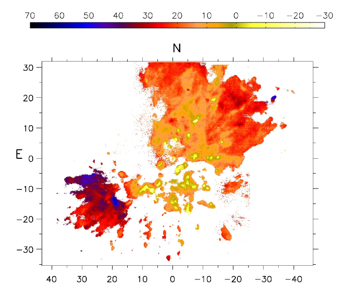
Figure 1: The velocity field for the full observed region of OMC1. (0,0) is the position of the Becklin-Neugebauer object (BN) 05^h35^m14$\aas@@fstack{s}$12, $-05\degr 22^{\prime}22\aas@@fstack{\prime\prime}9$ (J2000). Axes are labelled in arcseconds and colours represent radial velocities in $\,{\rm km\,s}^{-1}$. For the white regions no data are available.

We use the radial velocity map of the BN/KL region of the Orion Molecular Cloud (OMC1) of Gustafsson et al. (2003, 2006); Nissen et al. (2005). The data contain both brightness and velocity information and were obtained at the CFHT with a Fabry-Perot interferometer in conjunction with adaptive optics using the so-called GriF instrument (Clénet et al., 2002). Observations were performed in the NIR K-band by scanning the $v$=1-0 S(1) H₂ emission line at 2.121$\mu$m. The field of view is 36″$\times$ 36″and the pixel scale is 0$\aas@@fstack{\prime\prime}$035 where 1″$=460\,$AU. The dataset consists of four spatial and velocity resolved images, which are amalgamated into one field of 89″$\times$67″or 0.2$\times$0.15 pc for a distance of Orion of 460 pc (Bally et al., 2000). The field is centered approximately on the Becklin-Neugebauer (BN) object (05^h35^m14$\aas@@fstack{s}$1, $-05\degr 22\arcmin 22\aas@@fstack{\prime\prime}9$), see Fig. 1. The spatial resolution is 0$\aas@@fstack{\prime\prime}$15 (70 AU). The radial velocity at each spatial position was determined by the peak position in a lorentzian fit to the velocity profile provided by the Fabry-Perot. Relative velocities are determined with an accuracy of between $1\,{\rm km\,s}^{-1}$ (3$\sigma$) in the brightest regions and $8$–$9\,{\rm km\,s}^{-1}$ in the weakest regions considered here. Systematic errors due to mechanical instabilities in the Fabry-Perot may occur in establishing velocity differences between distant regions. As discussed in Gustafsson et al. (2006), tests have been performed to show that such systematic errors are not present in the data to any significant extent.

The emission of vibrationally excited H₂ observed here does not trace the bulk of the gas. Rather it traces hot, dense gas, where excitation occurs largely through shock excitation. Detailed models (Störzer & Hollenbach, 1999) show that the maximum brightness in the H₂ $v$=1–0 s(1) line from fluorescence in this region of OMC1 does not exceed 10–15% of the total brightness observed (Kristensen et al., 2003). Thus photon excitation is a minor contributor to the total brightness.

2.2 Results from observations

Since observational data provide only radial velocities in the plane of the sky in a 2D projection of the gas motions, we obtain only the transversal structure functions, as described earlier. Furthermore the accuracy of the velocity data in any pixel depends on the brightness in that pixel. Gustafsson et al. (2006) showed that more robust structure functions are obtained when the velocity differences are weighted by the brightness. On this basis we use a modified definition of the structure functions:

$$S_{p}(r)=\langle B(\@vec{x})B(\@vec{x}-\@vec{r})\,|v(\@vec{x})-v(\@vec{x}-\@vec{r})|^{p}\rangle.$$ (4)

Here $v$ is the line of sight velocity and the average is extended over all spatial positions $\@vec{x}$ and all lags $\@vec{r}$ where $r=|\@vec{r}|$. $B(\@vec{x})$ is the brightness at position $\@vec{x}$. We thus weight each velocity difference by the product of the brightness of the two spatial positions involved, thereby giving more weight to the brightest regions which exhibit the highest accuracy in the radial velocity.

The third order structure function of OMC1, $S_{3}(r)$, is displayed in Fig. 2a. It is not well represented by a single power law showing a clear deviation around 10³AU. This is also evident from the large variations in the local logarithmic derivatives of $S_{p}(r)$, shown in Fig. 2b for $p=1$–$5$, where the derivatives are evaluated numerically using a three-point formula. However, Benzi et al. (1993) discovered that the structure functions can be represented as functions of, say, the third order structure function, namely

$$S_{p}(r)\propto S_{3}(r)^{(\zeta_{p}/\zeta_{3})_{\rm ESS}}.$$ (5)

This is now known as extended self-similarity (ESS). Even if the structure functions of Eq. (1) are not power laws over any given range, the functions represented by Eq. (5) nevertheless exhibit good power law behaviour. The scaling in Eq. (5) is generally found to extend over a much larger range than for the structure functions of Eq. (1). As emphasized before, self-similarity, as expressed by Eq. (5), is believed to be more fundamental than the self-similar scaling with respect to $r$ (Benzi et al., 1993). In Fig. 2c we have plotted the ratio of the logarithmic slopes of $S_{p}$ and $S_{3}$, $d\ln S_{p}(r)/d\ln S_{3}(r)$, for $p=1$–$5$. If a range in which good power law scaling is present is encountered in the various structure functions, the ratio of logarithmic slopes should display plateaus in that range at values of $(\zeta_{p}/\zeta_{3})_{\rm ESS}$. From Fig. 2c we find that the structure functions for $p=1$–$5$ exhibit a reasonably good scaling range from $r=160\,$AU to $r=7000\,$AU. This range is marked by the dotted vertical lines in Fig. 2c. The scaling exponents are found by fits to Eq. (5) in this range. As an example we show in Fig. 2d the extended self-similarity plot of $S_{5}(r)$ vs. $S_{3}(r)$ together with the best fit yielding the slope $(\zeta_{p}/\zeta_{3})_{\rm ESS}=1.06$. The dotted lines mark the range of the fit. It is however clear from Fig. 2c that the scaling gets poorer when the order $p$ is increased. At $p=5$ the plateau is rather poorly defined (see also Fig. 2d) and therefore we cannot determine a scaling at higher orders than $p=5$. In Fig. 2e we show the scaling exponents $(\zeta_{p}/\zeta_{3})_{\rm ESS}$ vs. $p$ (+ signs) compared to the values predicted by the She-Leveque model of incompressible turbulence, Eq. (2) (dotted line) and the Boldyrev model of supersonic turbulence, Eq. (3) (dashed line). The scaling exponents derived from the velocity in OMC1 clearly deviate from both the She-Leveque and the Boldyrev scaling at $p\geq 4$. The OMC1 scaling exponents show signs of becoming constant at $(\zeta_{p}/\zeta_{3})_{\rm ESS}\sim 1$ or even slightly decreasing for $p>4$, in contrast to the theoretical scalings, which are monotonically increasing.

This result for velocities of hot, shocked gas in OMC1 at scales $70\,$AU – 3$\cdot 10^{4}$AU (3.4$\cdot 10^{-4}$pc to $0.15\,$ pc) differs from the findings of Padoan et al. (2003). They found that the density fields in the Perseus and Taurus molecular clouds as observed in CO follow Boldyrev scaling at scales larger than $0.08\,$pc.

Below we will show that the unusual scaling found here can be reproduced by numerical simulations of supersonic turbulence when only subsets of the simulations representing the shocked regions are considered.

Figure 2: a) Third order structure function of the velocities in OMC1. b) Logarithmic derivatives of $S_{p}(r)$ for $p=1$–$5$ c) Ratios of the differential slopes of $S_{P}(r)$ to the slope of the third order structure function for $p=1$–$5$. The vertical dotted lines mark the interval in which the scaling exponents have been fitted. d) $S_{5}(r)$ vs. $S_{3}(r)$. The dotted lines mark the range of the fit and the solid line is the best fit within that range yielding the logarithmic slope, $(\zeta_{p}/\zeta_{3})_{\rm ESS}=1.06$. e) The ESS scaling exponents (+) OMC1, (dotted line) She-Leveque scaling, (dashed line) Boldyrev scaling.

3 Simulations

In order to understand some of the peculiar scalings found in the observations we now consider data of supersonic isothermal compressible turbulence simulations. Such simulations have been performed by a number of different groups (Passot & Pouquet, 1987; Vazquez-Semadeni et al., 1995; Padoan et al., 1998; Klessen, 2000; Vázquez-Semadeni et al., 2003; Cho & Lazarian, 2003; Kritsuk & Norman, 2004). Here we consider simulations that are most closely related to those of Haugen et al. (2004b), except that magnetic fields are neglected here. The governing equations are

$${\partial\@vec{u}\over\partial t}+\@vec{u}\cdot\@vec{\nabla}\@vec{u}=-c_{\rm s}^{2}\@vec{\nabla}\ln\rho+\@vec{f}+{1\over\rho}\@vec{\nabla}\cdot\@vec{\tau},$$ (6)

$${\partial\ln\rho\over\partial t}+\@vec{u}\cdot\@vec{\nabla}\ln\rho=-\@vec{\nabla}\cdot\@vec{u},$$ (7)

where $\tau_{ij}=2\rho\nu{\sf S}_{ij}+\rho\mu\delta_{ij}\@vec{\nabla}\cdot\@vec{u}$ is the stress tensor and ${\sf S}_{ij}={1\over 2}(u_{i,j}+u_{j,i})-{1\over 3}\delta_{ij}u_{k,k}$ is the rate of strain matrix and commas denote partial differentiation. Following Nordlund & Galsgaard (1995), we assume $\mu$ to be proportional to the smoothed and broadened positive part of the negative divergence of the velocity, i.e.

$$\mu=c_{\rm shock}\left<\max_{5}[(-\@vec{\nabla}\@vec{u})_{+}]\right>,$$ (8)

where $c_{\rm shock}$ is the artificial viscosity parameter and the 5 underneath the $\max$ operator indicates that the maximum is taken over 5 by 5 by 5 mesh widths (or  ”pixels”). This is also the technique used by Padoan & Nordlund (2002) and Haugen et al. (2004b). The function $\@vec{f}$ denotes a random forcing function that consists of plane waves, normalized by a dimensionless amplitude factor $f_{0}$ that will be varied in the different simulations discussed below (see Appendix A).

The equations are solved on a periodic mesh of size $L^{3}$, where $L=2\pi/k_{1}$ is the length of the side of the box and $k_{1}$ is the smallest wave number in the domain. We use the Pencil Code, which is a high-order finite-difference code (sixth order in space and third order in time) for solving the compressible hydrodynamic equations.

We consider runs with different forcing amplitudes, $f_{0}$, leading to different root mean square Mach numbers, $\mbox{Ma}_{\rm rms}=u_{\rm rms}/c_{\rm s}$ where $c_{\rm s}$ is the speed of sound, see Table 1. The high resolution runs, in rows 2 and 3 of Table 1, have been evolved for about 40 sound travel times, $\tau_{\rm sound}=(c_{s}k_{1})^{-1}$, while the low resolution run has been conducted for about $90\,\tau_{\rm sound}$. The sound travel time can be associated with the turnover time by noting that $\tau_{\rm turn}=(u_{\rm rms}k_{1})^{-1}=\tau_{\rm sound}/\mbox{Ma}_{\rm rms}$.

Table 1: Parameters of the numerical simulations. Resolution, shock viscosity, forcing amplitude, Mach number, run time $\Delta t_{\rm run}$ in terms of turnover times $\tau_{\rm turn}$.

run	resolution	$c_{\rm shock}$	$f_{0}$	${\rm Ma}_{\rm rms}$	$\Delta t_{\rm run}/\tau_{\rm turn}$
1	$256^{3}$	2	2	3	270
2	$512^{3}$	3	10	7–9	320
3	$512^{3}$	2	10	8–10	360

3.1 Results from full 3D simulation

First, we show that the structure functions of the full 3D simulation follow the theoretical scaling of Boldyrev (2002). For a snapshot of Run 1 at $t=70\,\tau_{\rm sound}$ (corresponding to $t=210\,\tau_{\rm turn}$) we have calculated the longitudinal and transversal structure functions of the 3D simulation using

$$S_{p,\rm long}(l) = \langle|u_{x}(x+l,y,z)-u_{x}(x,y,z)|^{p}\rangle,$$ (9)

$$S_{p,\rm trans}(l) = \langle|u_{y}(x+l,y,z)-u_{y}(x,y,z)|^{p}\rangle$$ (10)

$$+ \langle|u_{z}(x+l,y,z)-u_{z}(x,y,z)|^{p}\rangle,$$

as in Eq. (1).

Figure 3: a) The third order transversal structure function of Run 1. b) logarithmic derivatives of $S_{p}(r)$ for $p=1$–$5$ (in ascending order). c) Ratios of the differential slopes of the transversal structure functions of order 1-5 to the slope of the third order structure function. d) The ESS scaling exponents of the transversal structure function (+) and the longitudinal structure function (diamonds) compared to the She-Leveque scaling (dotted line) and the Boldyrev scaling (dashed line).

In Fig. 3a the third order transversal structure function is shown. The logarithmic derivatives of $S_{p,\rm trans}(l)$ (Fig. 3b) show no range of scales where plateaus (good power law scaling) are present. Note, however, that in these simulations $\zeta_{2}$ is closer to unity than $\zeta_{3}$. In Fig. 3c we have plotted the logarithmic slope of $S_{p,\rm trans}(l)$ vs. $S_{3,\rm trans}(l)$ for $p=1$–$5$, i.e. again using the method of extended self-similarity (ESS). A range of good scaling is now seen to be present over most of the dynamical range from 10–80 mesh widths. The longitudinal structure functions are nearly identical to the transversal and are not shown here. The scaling exponents found from fits to the structure functions in the interval of 10–80 are plotted in Fig. 3d for both the transversal structure functions (+) and the longitudinal structure functions (diamonds). Both the transversal and the longitudinal structure functions follow the velocity scaling for supersonic turbulence of Boldyrev (2002).

3.2 Scaling of subsets of the simulations

We now study structure functions of subsets of the simulations and select subsets that resemble best the physical properties of the observational data, that is being composed of preferentially shocked gas. Similar work has already been carried out by Kritsuk & Norman (2004). First, in order to compare the simulations to the observations, we need to project the simulated 3D velocity components onto a 2D map of only radial velocity. The radial velocity in each spatial position is found by averaging the density weighed $z$-component (say) of the velocity over the $z$-range. That is,

$$\overline{u}_{z}(x,y)=\left.\int_{z}\rho u_{z}\,{\rm d}z\right/\int_{z}\rho\,{\rm d}z.$$ (11)

We have checked that this expression yields the same values of velocities as the method adopted in the reduction of the observational data obtained with GriF. In the observations, the true H₂ line profile is convolved with the very much broader instrumental Lorentzian profile of the Fabry-Perot interferometer and the radial velocity is found from a Lorentzian fit. The same procedure has been used on simulated velocity profiles through convolution and fitting and it has been found in numerous tests that the velocities derived are essentially the same as the centroid velocities obtained via Eq. (11). In Fig. 4 (top left, marked ”all”) the resulting 2D map is shown for Run 1 at $t=50\,\tau_{\rm sound}$, corresponding to $t=150\,\tau_{\rm turn}$.

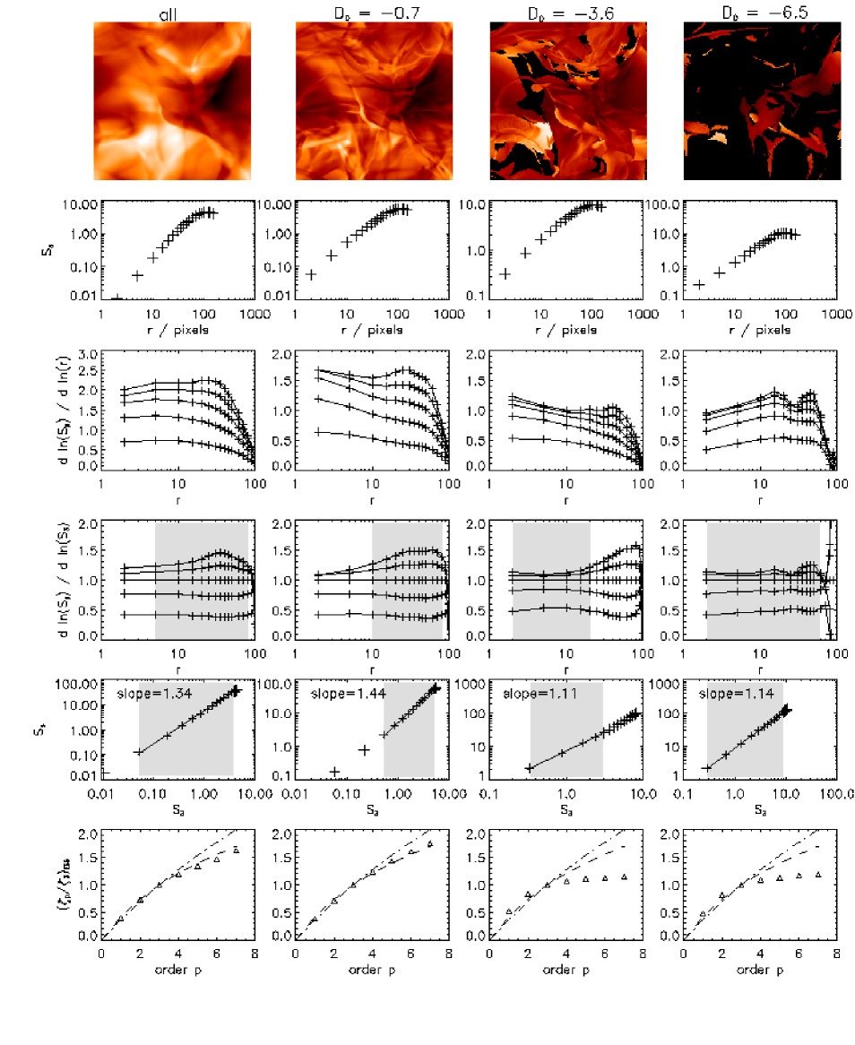
Figure 4: Run 1, $t=50\,\tau_{\rm sound}$. Results for projected maps including all points (1st column) and for subsets with $D_{0}=-0.7$, $-3.6$, and $-6.5$ (as marked), using $w=0.7$. Top row: radial velocity maps projected in the $z$-direction. Second row: third order structure functions averaged over 50 projection angles (see text). Third row: logarithmic derivatives of $S_{p}(r)$ for $p=1$–$5$ (in ascending order). Fourth row: ratios of differential slopes to $\zeta_{3}$ for order $p=1$–$5$. The grey shades indicate the ranges over which average values of $(\zeta_{p}/\zeta_{3})_{\rm ESS}$ are determined. Fifth row: $S_{5}(r)$ vs. $S_{3}(r)$. The ranges of grey shades correspond to those in the fourth row. Solid lines are best fits within the indicated ranges yielding the logarithmic slope, $(\zeta_{p}/\zeta_{3})_{\rm ESS}$. Bottom row: the radial velocity scaling compared to the She-Leveque scaling (dotted line) and the Boldyrev scaling (dashed line).

If the turbulence is homogeneous and isotropic the projected map should be independent of the projection angle. However, since the simulations have limited spatial extent, they turn out to show residual anisotropy, in the sense that independence of projection angle is not assured. Thus the projection map and subsequently the structure functions could depend on the projection angle. To minimize such effects we have calculated the structure functions for a number of random projection angles. An average of 50 angles was taken for Run 1. The higher resolution of Runs 2 and 3 should alleviate the problem of projection angle and averages over only 3 angles were taken in these cases. In the following all structure functions of projected maps refer to an average of structure functions. There could also be projection effects in the observations, but we have no choice but to ignore these.

The average third order structure function [Eq. (4) with $p=3$], the logarithmic derivatives of $S_{p}(r)$ for $p=1$–$5$, the ratio of the logarithmic slopes of $S_{p}(r)$ and $S_{3}(r)$, the extended self-similarity plot of $S_{5}(r)$ vs. $S_{3}(r)$, and the velocity scaling exponents are also shown in Fig. 4, passing down the left column, for the projected simulation of Run 1. In calculating the structure functions of the simulations we use $B=1$, that is, no brightness weighting in Eq. (4) since the velocities in the simulations are free of ‘observational’ errors. It is found that the scaling of the structure functions of the projected radial velocity follows that of Boldyrev, as did the transversal and longitudinal structure functions of the full 3D simulation (Fig. 3).

The problem is to identify the subset of structures in the simulations which corresponds to the structures represented in our observations. As mentioned above we observe a subset of the gas in OMC1 consisting very largely of shocked gas. In order to make comparison between observations and simulations it is therefore necessary to extract regions in the simulations where shocks occur. Shocks are generated where fast material attempts to overtake slower moving material and material shows rapid deceleration, that is, where a negative velocity gradient is present. In simulations, shocked regions can thus be distinguished as regions with suitably strong negative divergence ($\@vec{\nabla}\cdot\@vec{u}<0$), that is, convergence.

Thus, in order to compare with the observations, we choose different subsets of the simulations consisting of regions with shocks stronger than a certain degree. Kritsuk & Norman (2004) accomplished this by selecting regions where the density exceeds a certain threshold value. Here, on the other hand, we consider only regions that have stronger convergence than a given cut-off value, $D_{0}<$0. This is achieved by defining

$$D=\@vec{\nabla}\cdot\@vec{u}/\langle(\@vec{\nabla}\cdot\@vec{u})^{2}\rangle^{1/2}$$ (12)

as the relative velocity divergence, and the selection function $s$:

$$s(x,y,z)=\left\{\begin{array}[]{lllll}0&&\xi&\leq-1&\\ \textstyle{1\over 2}+\textstyle{1\over 4}\xi(3-\xi^{2})&\quad-1<&\xi&<1&\\ 1&&\xi&\geq 1,&\end{array}\right.$$ (16)

where $\xi=(D_{0}-D)/w$, and $w$ is the width of the selection function. All points with $D>D_{0}+w$, which we seek to exclude, have $s=0$. The selection function is chosen for its smooth variation between 0 and 1. We have used other somewhat different forms of the selection function and found that the results do not significantly depend on the specific form. Figure 5 shows an example of a local velocity field where shocks are present. The figure shows velocity vectors ($u_{x},u_{y}$) in an $xy$-plane and contours of shocked regions where $s>0$ for $D_{0}=-6.5$ and $w=0.7$ in Run 1.

The shock structure in an $xy$-slice of Run 3 is shown in Fig. 6, where regions with large negative values of $\@vec{\nabla}\cdot\@vec{u}$ (darker regions) represent shocks. The profiles of $u_{x}$, $u_{y}$, and $u_{z}$ are shown along a horizontal line on which the presence of a shock for example at $x=290$ is evident through large velocity changes in $u_{x}$, $u_{y}$, and $u_{z}$ over a range of only $\sim 5$ mesh widths. The higher Mach number of these simulations leads to larger velocity differences and stronger shocks compared to the simulations of Run 1.

The radial velocity in each spatial position $(x,y)$ is now found by a modified form of Eq. (11):

$$\overline{u}_{z}(x,y)=\left.\int_{z}s\rho u_{z}\,{\rm d}z\right/\int_{z}s\rho\,{\rm d}z.$$ (17)

Returning to Fig. 4, for a snapshot of Run 1 at $t=50\,\tau_{\rm sound}$ this shows maps projected in the $z$-direction as examples of subsets with $w=0.7$ and $D_{0}=-0.7$, $-3.6$, and $-6.5$. The value of $D$ in a region depends on how the velocity changes in the vicinity of that region. Large differences in velocity over a limited region lead to high values of $D$. Thus the restrictions on $D$ can be associated with typical minimum values of the velocity change that must occur in a shocked region for that region to be included in the structure function analysis. For example the physical interpretation of the restriction $D_{0}=-3.6$ is that in order for a pixel to be included there must be a velocity gradient in the immediate vicinity of that pixel, such that $|\Delta\@vec{u}|\sim 3\,{\rm km\,s}^{-1}$ over $\Delta r=10$ pixels. An estimate of the value of the gradient in physical units can be given by observing that the size of shocks in the simulations is typically 5 pixels. Assuming a physical shock width of C-shocks of 50 AU (Lacombe et al., 2004), the value of the required velocity gradient is $\sim 0.03\,{\rm km\,s}^{-1}\,{\rm AU}^{-1}$. When $D_{0}=-6.5$, typical values are $|\Delta\@vec{u}|\sim 5\,{\rm km\,s}^{-1}$ again over $\Delta r=10$ pixels. These values are estimated for Run 1 and are found to be higher in the runs with stronger forcing and higher Mach numbers for the same value of $D$.

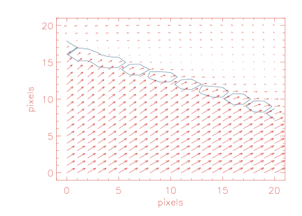
Figure 5: Vectorplot of ($u_{x},u_{y}$) in a section of an $xy$-plane in Run 1. Contours outline shocked regions where $s>0$ for the cut-off value $D_{0}=-6.5$, $w=0.7$, that is, regions where $D<-5.8$.

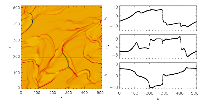
Figure 6: Left panel: $xy$-slice of $\@vec{\nabla}\cdot\@vec{u}$ through the box of Run 3 at some arbitrarily chosen value of $z$. The horizontal line indicates the location along which the profiles of $u_{x}$, $u_{y}$, and $u_{z}$ (in $\,{\rm km\,s}^{-1}$) are shown in the three panels on the right hand side. A strong shock is seen at $x=290$.

The map of $D_{0}=-0.7$, that is, including all shocked regions, displays sharp filamentary structure, compared with the map of all points in the simulation, which has smoother contours (see top row of Fig. 4). Excluding the weakest shocks, that is, for $D_{0}=-3.6$, leads to a more broken up appearance, and the filaments are clearly visible. When only the strongest shocks are considered, $D_{0}=-6.5$, the radial velocity map consists mostly of sheets and filaments.

Figure 4 also displays the third order structure functions for the three subsets as defined by values of $D_{0}$, as well as the logarithmic derivatives of $S_{p}(r)$, the ratio of the logarithmic slopes of $S_{p}(r)$ and $S_{3}(r)$, the extended self-similarity plot of $S_{5}(r)$ and $S_{3}(r)$, as well as the scaling exponents of the structure functions of the radial velocity. The structure functions are averages of 50 projected maps as described above. The third order structure function for the full simulation and the three subsets all display good power laws. The leveling off of the power laws at lags around 100 mesh widths is an artifact due to the finite size of the simulation of size 256. No bumps in the structure functions are seen. This is in marked contrast to the structure functions of the observations where clear bumps are present (see the first panel of Fig. 2).

The ratios of logarithmic slopes show plateaus over about an order of magnitude in scale, especially in the lower order structure functions, $p=1$, $2$. The scaling exponents $\zeta_{p}/\zeta_{3}$ are found by fits to Eq. (5) in the interval of $r$ where $d\ln S_{p}(r)/d\ln S_{3}(r)$ shows the best plateau. The plateau is found at $r=5$ to 80 mesh widths for the full simulation, at $r=10$ to 80 mesh widths for $D_{0}=-0.7$, at $r=2$ to 20 for $D_{0}=-3.6$ and at $r=2$ to 60 for $D_{0}=-6.5$. The ranges used for fitting are indicated in Fig. 4 with grey shading. The best power law fits to $S_{5}(r)$ vs. $S_{3}(r)$ in the indicated ranges are shown in the fifth row of Fig. 4. The value of the slope is indicated. The velocity scaling is close to following that of Boldyrev when all points in the simulation are included and when only shocked regions with $D<0$ ($D_{0}=-0.7$) are included. There is, however, a dramatic change in the scaling when the restrictions on the strength of the shocks are made tighter. For both $D_{0}=-3.6$ and $D_{0}=-6.5$ the scaling deviates strongly from both She-Leveque and Boldyrev scalings. This change in behaviour is associated with a shift in the range for which a plateau can be seen. Especially in the last column of Fig. 4 the scaling is seen to extend all the way from the resolution limit (2 mesh widths) to 60 mesh widths. This cannot be regarded as regular inertial range scaling because the usual dissipative subrange, always present in turbulence simulations, cannot be distinguished. We associate the apparent shift of the ranges with the presence of shock structures which become more strongly pronounced as the cutoff value, $D_{0}$, is moved to more negative values. Thus we are beginning to see effects due to the use of artificial viscosity when $D$ becomes sufficiently negative. These artificially smoothed shocks may resemble C-type shocks that occur in the magnetized interstellar medium and are known to be a common feature in OMC1 (Gustafsson et al., 2003; Nissen et al., 2005). We also note that the nominal dissipation scale without artificial viscosity is just 1–2 mesh widths, which is still below the artificial dissipation scale of the shocks of $\sim$ 5 or more mesh widths. The scaling is seen to remain nearly constant for $p\geq 3$, resembling the scaling found in the observations of OMC1. This is qualitatively similar to the results of Kritsuk & Norman (2004), who found systematically smaller scaling exponents for $p>3$ when only high density regions are considered. This shows that the unusual scaling observed in OMC1 can be the effect of observing only the hot, shocked gas, and that hydrodynamical turbulence simulations without self-gravity or magnetic fields are able to reproduce this.

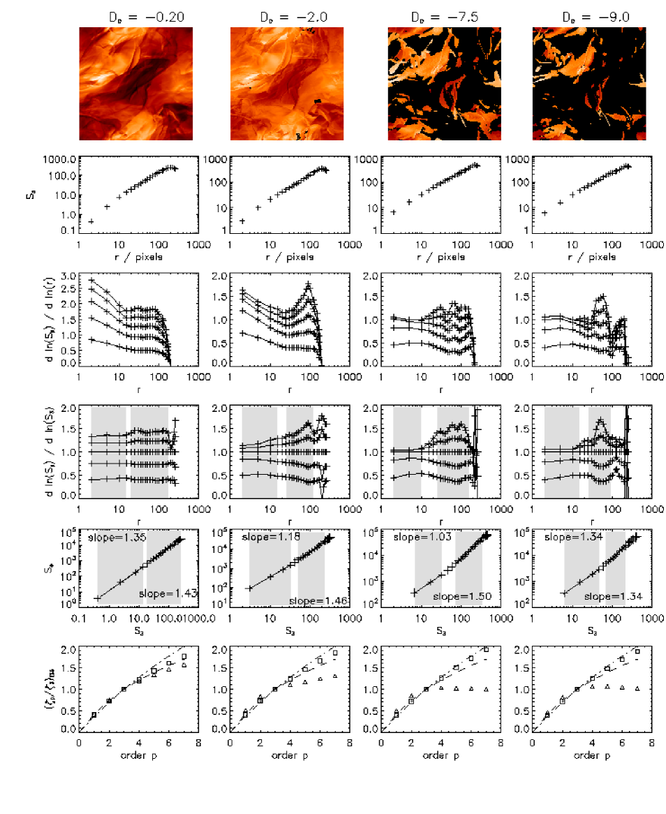
Figure 7: Run 3, $t=39\,\tau_{\rm sound}$. Results for projected maps for subsets with $w=0.20$ and $D_{0}=-0.20$, $-2.0$, $-7.5$ and $-9.0$. Top row: radial velocity maps projected in the $z$-direction. Second row: third order structure functions averaged over 3 projection angles (see text). Third row: logarithmic derivatives of $S_{p}(r)$ for $p=1$–$5$ (in ascending order). Fourth row: ratios of differential slopes to $\zeta_{3}$ for order $p=1$–$5$. The grey shades indicate the ranges over which average values of $(\zeta_{p}/\zeta_{3})_{\rm ESS}$ are determined. Fifth row: $S_{5}(r)$ vs. $S_{3}(r)$. The ranges of grey shades correspond to those in the fourth row. Solid lines are best fits within the indicated ranges yielding the logarithmic slope, $(\zeta_{p}/\zeta_{3})_{\rm ESS}$. Bottom row: the radial velocity scaling compared to the She-Leveque scaling (dotted line) and the Boldyrev scaling (dashed line). $\triangle$: large scales, $\Box$: small scales.

Figure 7 shows similar results to Fig. 4 but for a snapshot of Run 3 at $t=39\,\tau_{\rm sound}$. The subsets corresponding to $D_{0}=-0.20$, $-2.0$, $-7.5$, and $-9.0$ show the same trends as seen in Fig. 4. The tighter the restrictions on the strength of the shocks, the sharper and more broken up the filamentary structures become. The radial velocity scaling flattens strongly when $D_{0}=-7.5$ and $-9.0$ (bottom row in Fig. 7).

The grey-shaded areas in the fourth row of Fig. 7 indicate two different regions where scaling can tentatively be noted, in contrast to the single regions identified in Fig. 4. As noted earlier, the dissipation scale for low velocity gradients is essentially given by 1–2 mesh widths. This is equivalent to the case in which no artificial viscosity is introduced; see Eq. (8). The dissipation scale rises to 5 or more mesh widths in locations where large velocity gradients are encountered. The two different scales identified in Fig. 7 (rows 4 and 5) have dimensions of 2 to $>$10 mesh widths and 30 to $>$100 meshwidths. The smaller of these ranges covers that associated with artificial viscosity. The scaling at the lower range will thus be affected by the presence of shocks. This may take place through the locally enhanced viscosity embodied in Eq. (8).

We now consider the scaling associated with the two different regions separately. In Fig. 7, open triangles refer to the larger regions and open squares to the smaller regions. For the data in the left column for $D_{0}=-0.20$, where all regions with a positive value of the convergence are included, that is, all shocks, it is seen that both scaling regions (small scales, 2–15 mesh widths, and large scales, 20–170 mesh widths) show scaling behaviour roughly compatible with Boldyrev scaling. When we introduce more restrictive thresholds for $D_{0}$ different behaviour is found. The large scales then begin to follow more closely the standard She-Leveque scaling. At the same time, the small scales, associated with shocks, show the levelling off discussed in connection with Fig. 4 for strongly shocked regions, and as seen in the observations, Fig. 2e. We therefore are able to explain the unexpected scaling found in the observations through an inherent selection of shocked regions.

We note that with the greater energy dissipation associated with Run 2, slopes for small and large scales differ as for Run 3 but less markedly.

Figure 8: Run 2, $t=37\,\tau_{\rm sound}$. Third order structure functions of projected maps with $w=0.2$ and $D_{0}=-5.1$ and $D_{0}=-7.5$.

3.3 Non-power law behaviour in structure functions

The structure functions of Run 3 (second row in Fig. 7) are all well represented by power laws in contrast to the behaviour found in the structure functions of OMC1 (Fig. 2). In one snapshot of Run 2, however, similar bumps to those in the observations are detected; see Fig. 8. The deviations from power laws of the structure functions in Run 2 are found in subsets with high values of the threshold, $D_{0}$, in the snapshot at $t=37\,\tau_{\rm sound}$. Examples are seen in Fig. 8 for $D_{0}=-5.1$ and $D_{0}=-7.5$ where it is clear that the third order structure functions displays bumps around 20 and 60 mesh widths. Other snapshots of Run 2 however do not show this feature. The bumps in the structure functions indicate the presence of preferred scale sizes in the simulation. This means that even if the starting point is a fully isotropic hydrodynamic solution of supersonic turbulence, then preferred scales can be encountered by selecting shocked regions that have a typical filamentary length of some hundred mesh widths (see Fig. 6).

4 Conclusion

We have used observational data of shocked H₂ emission in OMC1 to show that structure functions at scales 70 – 3$\cdot 10^{4}\,$AU (3.4$\cdot 10^{-4}$ – 0.15 pc) exhibit unusual scaling exponents for $p>3$. The scaling exponents are nearly constant for $p>3$ and smaller than predicted by both She & Leveque (1994) and Boldyrev (2002).

In three simulations we have selected shocked regions by imposing requirements on the value of the velocity divergence, $\@vec{\nabla}\cdot\@vec{u}$. In certain important respects the simulations presented here are then remarkably successful in reproducing the statistical behaviour observed in OMC1. In other equally important areas, they fail. Let us first reiterate the success.

We have found that by only including shocks that are relatively strong ($D_{0}<-1.5$), the unusual scaling exponents of the observations are reproduced in the simulations. By contrast, a scaling following that of She & Leveque (1994) or Boldyrev (2002) is found when all points in the simulations are included in the data. An explanation for this behaviour is as follows. Enhanced energy content at small scales, relative to larger scales, implies smaller slopes, that is, smaller values of $\zeta_{p}$. Both the observational data of OMC1, and some of those subsets of the simulations selected only to include shocks, show that the values of $\zeta_{p}$ are reduced for $p\geq 4$. Since structure functions of high order $p$ are dominated by regions of strong velocity differences, it follows that the observed excess of small scale energy is associated with regions of large velocity differences. These are likely to be the regions of strong shocks, as is evidenced by the fact that reduced values of $\zeta_{p}$ are most clearly seen in subsets of the simulations that select the most strongly convergent high density regions.

The present work does not however furnish any explanation of why departure from the She-Leveque or Boldyrev scaling occurs at the specific value of $p\geq 4$. It is possible that the critical value of $p$ is in some way connected with the physical nature of the shocks, for example the fact that they are smoothed in the simulations, mimicking the structure of continuous (C-) type shocks, rather than jump (J-) type shocks (Flower et al., 2003, and references therein).

We now turn to the failure of the simulations. The structure functions of the observations in OMC1 all deviate from power laws and exhibit clear bumps around $10^{3}$AU, exemplified by the third order structure function in Fig. 2. This cannot in general be reproduced by the simulations. There appears to be two possible explanations for this observed behaviour. The first is that the deviation from power laws is due to protostar formation and associated outflows at a preferred scale. The second is that the behaviour is in some way inherent in the nature of the turbulence as opposed to the presence of protostars.

Turning to the first suggestion, the process of star formation pulls structure of a certain size out of the cascade and creates outflows, injecting energy into a turbulent background. Gravitational energy and angular momentum is spewed out of the star via such outflows and turned into local turbulence, hence increasing the overall turbulent content of the gas – and restarting the whole cascade process. Such outflows are of course not present in the simulations.

The second suggestion, that the deviation from power law is somehow inherent in the nature of the turbulence, requires that there is some non-statistical element in this medium which is otherwise governed by statistical considerations. This may arise through our selection of strong shocks as a subset of the whole. We have seen in Fig.8 that traces of bumps in the structure functions are found in one snapshot of Run 2 when highly shocked material is selected. The deviations of the structure functions from power laws are not as pronounced in the simulation as in the observations of OMC1. However this finding provides some evidence that part of the explanation for the deviations from power laws of the structure functions in OMC1 arises from the fact that we observe preferentially shocked gas. As departures from power law behaviour are only evident in a single snapshot and not throughout the simulation at other times, this suggestion remains tentative.

In order to explore the reasons for the departure from power law behaviour, more advanced simulations are necessary. These should include self-gravity and energy feedback from protostellar zones through outflows and should ultimately incorporate ionization and magnetic fields.

Appendix A The forcing function

For completeness we specify here the forcing function used in the present paper. It is defined as (Brandenburg, 2001)

$$\@vec{f}(\@vec{x},t)={\rm Re}\{N\@vec{f}_{\@vec{k}(t)}\exp[{\rm i}\@vec{k}(t)\cdot\@vec{x}+{\rm i}\phi(t)]\},$$ (18)

where $\@vec{x}$ is the position vector. The wavevector $\@vec{k}(t)$ and the random phase $-\pi<\phi(t)\leq\pi$ change at every time step, so $\@vec{f}(\@vec{x},t)$ is $\delta$-correlated in time. For the time-integrated forcing function to be independent of the length of the time step $\delta t$, the normalization factor $N$ has to be proportional to $\delta t^{-1/2}$. On dimensional grounds it is chosen to be $N=f_{0}c_{\rm s}(|\@vec{k}|c_{\rm s}/\delta t)^{1/2}$, where $f_{0}$ is a nondimensional forcing amplitude. At each timestep we select randomly one of many possible wavevectors with length between 1 and 2 times the minimum wavenumber in the box, $k_{1}$. The average wavenumber is $k_{\rm f}=1.5k_{1}$. We force the system with transverse non-helical waves,

$$\@vec{f}_{\@vec{k}}=\left(\@vec{k}\times\@vec{e}\right)/\sqrt{\@vec{k}^{2}-(\@vec{k}\cdot\@vec{e})^{2}},$$ (19)

where $\@vec{e}$ is an arbitrary unit vector not aligned with $\@vec{k}$; note that $|\@vec{f}_{\@vec{k}}|^{2}=1$.

References

- Anselmet et al. (1984) Anselmet, F., Gagne, Y., Hopfinger, E. J., & Antonia, R. A. 1984, J. Fluid Mech., 140, 63
- Bally et al. (2000) Bally, J., O’Dell, C. R., & McCaughrean, M. J. 2000, AJ, 119, 2919
- Bensch et al. (2001) Bensch, F., Stutzki, J., & Ossenkopf, V. 2001, A&A, 366, 636
- Benzi et al. (1993) Benzi, R., Ciliberto, S., Tripiccione, R., et al. 1993, Phys. Rev. E, 48, 29
- Boldyrev (2002) Boldyrev, S. 2002, ApJ, 569, 841
- Boldyrev et al. (2002a) Boldyrev, S., Nordlund, Å., & Padoan, P. 2002a, ApJ, 573, 678
- Boldyrev et al. (2002b) Boldyrev, S., Nordlund, Å., & Padoan, P. 2002b, Phys. Rev. Lett., 89, 031102
- Brandenburg (2001) Brandenburg, A. 2001, ApJ, 550, 824
- Cho & Lazarian (2003) Cho, J. & Lazarian, A. 2003, MNRAS, 345, 325
- Clénet et al. (2002) Clénet, Y., Le Coarer, E., Joncas, G., et al. 2002, PASP, 114, 563
- Dubrulle (1994) Dubrulle, B. 1994, Phys. Rev. Lett., 73, 959
- Elmegreen & Scalo (2004) Elmegreen, B. G. & Scalo, J. 2004, ARA&A, 42, 211
- Falgarone et al. (1994) Falgarone, E., Lis, D. C., Phillips, T. G., et al. 1994, ApJ, 436, 728
- Falgarone & Phillips (1990) Falgarone, E. & Phillips, T. G. 1990, ApJ, 359, 344
- Falgarone et al. (1995) Falgarone, E., Pineau des Forets, G., & Roueff, E. 1995, A&A, 300, 870
- Flower et al. (2003) Flower, D. R., Le Bourlot, J., Pineau des Forêts, G., & Cabrit, S. 2003, MNRAS, 341, 70
- Frick et al. (1995) Frick, P., Dubrulle, B., & Babiano, A. 1995, Phys. Rev. E, 51, 5582
- Frisch (1995) Frisch, U. 1995, Turbulence. The legacy of A.N. Kolmogorov (Cambridge: Cambridge University Press)
- Goodman et al. (1998) Goodman, A. A., Barranco, J. A., Wilner, D. J., & Heyer, M. H. 1998, ApJ, 504, 223
- Gustafsson et al. (2006) Gustafsson, M., Field, D., Lemaire, J. L., & Pijpers, F. P. 2006, A&A, 445, 601
- Gustafsson et al. (2003) Gustafsson, M., Kristensen, L. E., Clénet, Y., et al. 2003, A&A, 411, 437
- Haugen et al. (2004a) Haugen, N. E., Brandenburg, A., & Dobler, W. 2004a, Phys. Rev. E, 70, 016308
- Haugen et al. (2004b) Haugen, N. E. L., Brandenburg, A., & Mee, A. J. 2004b, MNRAS, 353, 947
- Joulain et al. (1998) Joulain, K., Falgarone, E., Des Forets, G. P., & Flower, D. 1998, A&A, 340, 241
- Kerr et al. (2001) Kerr, R. M., Meneguzzi, M., & Gotoh, T. 2001, Physics of Fluids, 13, 1985
- Klessen (2000) Klessen, R. S. 2000, ApJ, 535, 869
- Kolmogorov (1941) Kolmogorov, A. N. 1941, Dokl. Akad. Nauk, 30, 301
- Kristensen et al. (2003) Kristensen, L. E., Gustafsson, M., Field, D., et al. 2003, A&A, 512, 727
- Kritsuk & Norman (2004) Kritsuk, A. G. & Norman, M. L. 2004, ApJ, 601, L55
- Lacombe et al. (2004) Lacombe, F., Gendron, E., Rouan, D., et al. 2004, A&A, 417, L5
- Larson (1981) Larson, R. B. 1981, MNRAS, 194, 809
- Lis et al. (1998) Lis, D. C., Keene, J., Li, Y., Phillips, T. G., & Pety, J. 1998, ApJ, 504, 889
- Miesch & Bally (1994) Miesch, M. S. & Bally, J. 1994, ApJ, 429, 645
- Miesch et al. (1999) Miesch, M. S., Scalo, J., & Bally, J. 1999, ApJ, 524, 895
- Nissen et al. (2005) Nissen, H., Gustafsson, M., Lemaire, J., et al. 2005, to appear in A&A, astro-ph/0511226
- Nordlund & Galsgaard (1995) Nordlund, Å. & Galsgaard, K. 1995, a 3D MHD code for Parallel Computers; http://www.astro.ku.dk/~aake/NumericalAstro/papers/kg/mhd.ps.gz
- Ossenkopf & Mac Low (2002) Ossenkopf, V. & Mac Low, M.-M. 2002, A&A, 390, 307
- Padoan et al. (1999) Padoan, P., Bally, J., Billawala, Y., Juvela, M., & Nordlund, Å. 1999, ApJ, 525, 318
- Padoan et al. (2003) Padoan, P., Boldyrev, S., Langer, W., & Nordlund, Å. 2003, ApJ, 583, 308
- Padoan et al. (2004) Padoan, P., Jimenez, R., Nordlund, Å., & Boldyrev, S. 2004, Phys. Rev. Lett., 92, 191102
- Padoan et al. (1998) Padoan, P., Juvela, M., Bally, J., & Nordlund, A. 1998, ApJ, 504, 300
- Padoan & Nordlund (2002) Padoan, P. & Nordlund, Å. 2002, ApJ, 576, 870
- Passot & Pouquet (1987) Passot, T. & Pouquet, A. 1987, J. Fluid Mech., 181, 441
- Pety & Falgarone (2000) Pety, J. & Falgarone, É. 2000, A&A, 356, 279
- Pety & Falgarone (2003) Pety, J. & Falgarone, E. 2003, A&A, 412, 417
- Politano & Pouquet (1995) Politano, H. & Pouquet, A. 1995, Phys. Rev. E, 52, 636
- Rosenthal et al. (2000) Rosenthal, D., Bertoldi, F., & Drapatz, S. 2000, A&A, 356, 705
- She & Leveque (1994) She, Z. & Leveque, E. 1994, Phys. Rev. Lett., 72, 336
- Störzer & Hollenbach (1999) Störzer, H. & Hollenbach, D. 1999, ApJ, 515, 669
- Vázquez-Semadeni et al. (2003) Vázquez-Semadeni, E., Ballesteros-Paredes, J., & Klessen, R. S. 2003, ApJ, 585, L131
- Vazquez-Semadeni et al. (1995) Vazquez-Semadeni, E., Passot, T., & Pouquet, A. 1995, ApJ, 441, 702