Simulating Cosmic Reionization at Large Scales I: the Geometry of Reionization

Abstract

We present the first large-scale radiative transfer simulations of cosmic reionization, in a simulation volume of $(100\,h^{-1}\rm Mpc)^{3}$. This is more than a 2 orders of magnitude improvement over previous simulations. We achieve this by combining the results from extremely large, cosmological, N-body simulations with a new, fast and efficient code for 3D radiative transfer, $\rm C^{2}$-Ray, which we have recently developed. These simulations allow us to do the first numerical studies of the large-scale structure of reionization which at the same time, and crucially, properly take account of the dwarf galaxy ionizing sources which are primarily responsible for reionization. In our realization, reionization starts around $z\sim 21$, and final overlap occurs by $z\sim 11$. The resulting electron-scattering optical depth is in good agreement with the first-year WMAP polarization data. We show that reionization clearly proceeded in an inside-out fashion, with the high-density regions being ionized earlier, on average, than the voids. Ionization histories of smaller-size (5 to 10 comoving Mpc) subregions exabit a large scatter about the mean and do not describe the global reionization history well. This is true even when these subregions are at the mean density of the universe, which shows that small-box simulations of reionization have little predictive power for the evolution of the mean ionized fraction. The minimum reliable volume size for such predictions is $\sim 30$ Mpc. We derive the power-spectra of the neutral, ionized and total gas density fields and show that there is a significant boost of the density fluctuations in both the neutral and the ionized components relative to the total at arcminute and larger scales. We find two populations of H II regions according to their size, numerous, mid-sized ($\sim 10$ Mpc) regions and a few, rare, very large regions tens of Mpc in size. Thus, local overlap on fairly large scales of tens of Mpc is reached by $z\sim 13$, when our volume is only about 50% ionized, and well before the global overlap. We derive the statistical distributions of the ionized fraction and ionized gas density at various scales and for the first time show that both distributions are clearly non-Gaussian. All these quantities are critical for predicting and interpreting the observational signals from reionization from a variety of observations like 21-cm emission, Ly-$\alpha$ emitter statistics, Gunn-Peterson optical depth and small-scale CMB secondary anisotropies due to patchy reionization.

1 Introduction

Understanding the large-scale geometry of reionization (sometimes also referred to as topology of reionization), i.e. the size- and spatial distribution of the ionized and neutral patches, and their evolution in time is one of the most important problems in this fast-developing field. Better understanding of this geometry is crucial for making detailed and realistic predictions for the observational features of reionization. Detecting these features is the goal of a number of upcoming meter-wavelength radio synthesis telescopes, such as PAST, LOFAR, MWA, and SKA. Also being planned are observations of small-scale CMB anisotropies created by ionized patches (e.g. Santos et al. 2003), and direct observations of high-redshift Ly-$\alpha$ emitters and their clustering using either James Webb Space Telescope or ground-based telescopes (e.g. Malhotra & Rhoads 2004; Stern et al. 2005). Such observations can in principle map the complete progress of reionization through time and space.

In the last few years a variety of different cosmological radiative transfer methods have been developed. These generally fall into two basic groups, moment methods (Gnedin & Abel 2001; Cen 2002; Hayes & Norman 2003), and ray-tracing methods (Mellema et al. 1998; Razoumov & Scott 1999; Abel et al. 1999; Ciardi et al. 2000; Nakamoto et al. 2001; Sokasian et al. 2001; Razoumov et al. 2002; Lim & Mellema 2003; Maselli et al. 2003; Shapiro et al. 2004; Bolton et al. 2004; Iliev et al. 2005b; Mellema et al. 2006a). Several simulations of reionization have been performed using some of these codes, most often as a post-processing step (i.e. the “static limit” which neglects the gasdynamical response to photoionization and heating) to cosmological N-body simulations with and without gas (Nakamoto et al. 2001; Sokasian et al. 2001; Razoumov et al. 2002; Maselli et al. 2003), while others directly coupled the radiative transfer to the gas evolution and followed the evolution self-consistently (Gnedin & Abel 2001). Despite these significant advances, all current reionization simulations are limited to fairly small volumes, with computational box sizes not exceeding $20\,h^{-1}$ comoving Mpc, and usually much smaller than that. The main reason for this limitation is that the ionizing photon output during reionization is dominated by dwarf galaxies, which at early times are far more numerous than the larger galaxies, while the ionizing photon consumption (ionizations and recombinations) is dominated by even smaller structures, due to the hierarchical nature of $\Lambda$CDM structure formation. The need to resolve such small galaxies imposes a severe limit on the computational box size. On the other hand, these ionizing sources were strongly clustered at high redshift and, as a consequence, the H II regions they created are expected to quickly overlap and grow to very large sizes, reaching up to tens of Mpc (e.g. Barkana & Loeb 2004; Furlanetto & Oh 2005; Cen 2005; Iliev et al. 2005c). The many orders of magnitude of difference between these scales demand extremely high resolution from any simulations designed to study early structure formation from the point of view of reionization. Further limitations are imposed by the low efficiency of the used radiative transfer methods. Most methods are based on ray-tracing and thus are quite accurate, but their computational expense grows roughly proportionally to the number of ionizing sources present. This generally renders them impractical when more than a few thousand ionizing sources are involved, severely limiting the computational volume that can be simulated effectively.

Over the years many analytical approaches to modelling reionization have been proposed (e.g. Shapiro et al. 1994; Haiman & Holder 2003; Wyithe & Loeb 2003; Furlanetto et al. 2004; Iliev et al. 2005a). However, these models are all statistically-averaged ones and can thus only make statistical predictions. Moreover, they have not been checked against simulations or observations and hence their level of reliability is currently unclear. In general, semi-analytical models are inevitably simplified in order to render the problem tractable and their prediction power depends on how well they can represent the relevant features of reionization. They could be quite useful in situations when simulations are too expensive, e.g. for exploring the parameter space, or studying very rare objects which requires huge volumes, well beyond the reach of current simulations. However, the correctness, reliability, and limitations of any semi-analytical model should still be established first by comparison with simulations.

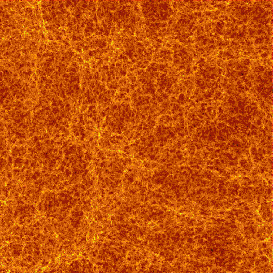
Figure 1: Early structure formation in $\Lambda$CDM, at $z=10$, from our N-body simulation: projection of the cloud-in-cell densities on the fine simulation grid ($3248\times 3248$ pixels) in a 20 comoving Mpc slice ($\sim 6\times 10^{8}$ particles in the slice) of the $(100\,h^{-1})^{3}$ Mpc³ simulation volume. (See $\tt http://www.cita.utoronto.ca/\!\sim\!iliev/research.html$ for the full-resolution images and some movies of our simulations).

The current development of novel, more efficient codes for both cosmological N-body and hydrodynamical simulations and for numerical radiative transfer finally allows reionization simulations in large volumes. In this work we present the first large-scale, in a volume of $(100\,h^{-1}\rm Mpc)^{3}$, radiative transfer simulations of this process. We achieve this by combining the results from an extremely large N-body simulation performed with the code PMFAST (Merz et al. 2005) with a very fast and efficient cosmological radiative transfer code called $C^{2}$-Ray which we have recently developed (Mellema et al. 2006a). Our underlying N-body simulation has a sufficient mass resolution to resolve all halos down to dwarf galaxies inside our volume reliably, as well as their clustering and the relevant large-scale fluctuations of the density field. Our new ray-tracing radiative transfer method is based on explicit photon conservation in space and time which allows us to use large time steps and fairly coarse grids without loss of accuracy. Ionization fronts (I-fronts) are correctly tracked even for very optically-thick cells. These features make our code far more efficient than previous ones, allowing for faithful treatment (using parallel machines) of tens, even hundreds of thousands of ionizing sources on much larger grids than before.

We also note the very recent results of Kohler et al. (2005b, a) which simulate extremely large cosmological volumes, up to $\sim 1$ Gpc in size. However, these simulations have very coarse resolutions and do not resolve the individual ionizing sources. These are instead represented only in a mean, approximate way based on separate, much smaller scale radiative transfer simulations. Such approach may be appropriate for certain problems, like the one discussed in these papers, namely modelling the rare, bright high-redshift QSO’s. However it cannot be used to answer the questions posed and addressed in the present work, due to its approximate nature and lack of both a source population resolution and a spatial one.

We assume that the gas is closely following the dark matter distribution, which is a quite accurate assumption at the large scales considered here (Zhang et al. 2004). Furthermore, the gas back reaction due to the ionization can be ignored to a good approximation at these scales since the global, large-scale I-fronts are highly supersonic, of weak R-type (from “rarefied”, i.e. typically occurring in low-density gas), out-running any reaction of the gas (Shapiro & Giroux 1987). This approximation breaks down in dense gas inside halos, where the I-fronts slow down and transform to a D-type (from “dense”, i.e. typically occurring in dense gas), generally preceded by a shock (Shapiro et al. 2004; Iliev et al. 2005b). Thus, on smaller scales a fully-coupled hydrodynamic and radiative transfer treatment is required.

The general outlay of this paper is as follows. We describe our numerical methodology in § 2. In § 3 we present our results: on the globally-averaged quantities (e.g. ionized fraction, mean number of recombinations per atom, electron scattering optical depth) in § 3.1 and on the reionization geometry in § 3.2. Finally, we discuss our results in § 4. This paper concentrates on the geometry of reionization, the corresponding implications for the observation of the 21-cm signal will be presented in a companion paper (Mellema et al. 2006b).

Throughout this study we assume a flat $\Lambda$CDM cosmology with parameters ($\Omega_{m},\Omega_{\Lambda},\Omega_{b},h,\sigma_{8},n)=(0.27,0.73,0.044,0.7,0.9,1)$ (Spergel et al. 2003), where $\Omega_{m}$, $\Omega_{\Lambda}$, and $\Omega_{b}$ are the total matter, vacuum, and baryonic densities in units of the critical density, $h$ is the Hubble constant in units of 100 $\rm km\,s^{-1}Mpc^{-1}$, $\sigma_{8}$ is the standard deviation of linear density fluctuations at present on the scale of $8\rm h^{-1}{\rm Mpc}$, and $n$ is the index of the primordial power spectrum. We use the CMBfast transfer function (Seljak & Zaldarriaga 1996).

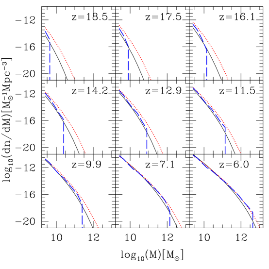
Figure 2: Halo mass function from our simulation at various redshifts, as labeled, (thick, long-dashed) and analytical approximations: the standard Press-Schechter (PS; thin, solid) and Sheth-Tormen (ST; thick, dotted).

2 The Simulations

2.1 N-body simulations

We performed the underlying cosmological N-body simulations with the particle-mesh cosmological code PMFAST (Merz et al. 2005) with simulation volume of $(100\,\rm h^{-1}Mpc)^{3}$. Our resolution is $1624^{3}=4.28$ billion dark matter particles and $3248^{3}$ computational cells (Figure 1). The particle mass is $2.5\times 10^{7}M_{\odot}$ and in order to be conservative we consider only well-resolved halos which contain at least 100 particles. This gives a minimum halo mass of $2.5\times 10^{9}M_{\odot}$, corresponding to dwarf galaxies. We find the halos and their detailed parameters “on-the-fly”, while the simulation is running, using a spherical overdensity method with overdensity of $\delta=130$ (although the results do not depend significantly on the particular overdensity value we have chosen). The first halos form at $z\approx 21$ and the number of halos quickly rises thereafter, reaching over 85,000 halos by $z\sim 11$ and over 0.8 million halos by $z=6$. In Figure 2 we plot several sample halo mass functions from our simulation at different redshifts. At lower redshifts ($z\mathrel{\hbox{\hbox to0.0pt{\hbox{\lower 4.0pt\hbox{$\sim$}}\hss}\hbox{$<$}}}10$) our mass function is in excellent agreement with the analytical Sheth-Tormen (ST) mass function (e.g. Sheth & Tormen 2002), while at higher redshifts the ST mass function somewhat overestimates the actual number of halos. The standard Press-Schechter approximation (PS; Press & Schechter 1974), on the other hand, significantly underestimates the number of rare halos in the exponential tail of the mass function but agrees fairly well with the numerical mass function (as well as with the ST mass function) for less rare halos. Previously, Reed et al. (2003) found a similar trend of ST overestimating the mass function at $z>10$, but being fairly accurate at later times. We will present the detailed results from a series of these simulations with several different computational volume sizes in a separate paper.

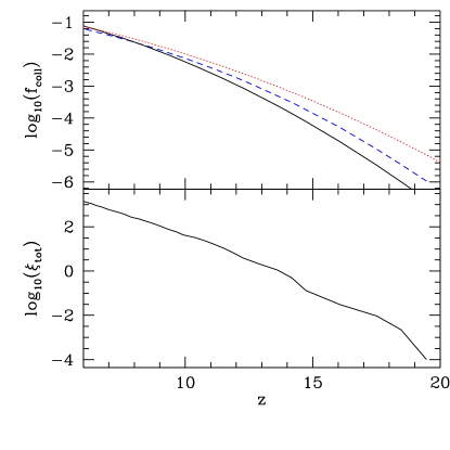
Figure 3: (top) Collapsed mass fraction in halos in the simulation, $f_{\rm coll}$ (dashed), and the analytical PS (solid) and ST (dotted) halo collapsed fractions with the same minimum halo mass, and (bottom) cumulative number of ionizing photons per hydrogen atom, $\xi_{\rm tot}$ emitted by all sources in the computational volume.

2.2 Reionization simulations

We performed our radiative transfer simulations using the cosmological ray-tracing radiative transfer code $C^{2}$-Ray (Mellema et al. 2006a). The PMFAST N-body simulation described above provided the density fields and the halo catalogues containing the masses, positions and other detailed properties of the collapsed halos. We have saved 50 of these density fields (of the $812^{3}$ coarse PMFAST density field), spaced at roughly equal time intervals, $\Delta t_{i}\approx 20$ Myr, and the corresponding halo catalogues. The density field is further re-gridded, to $406^{3}$ and $203^{3}$ computational cells, for radiative transfer runs at different resolutions. We assume that the gas density distribution follows that of the dark matter. This is a quite accurate assumption at the large scales considered in these simulations (Zhang et al. 2004). In the interest of speed and manageability of the calculations, we assume a fixed temperature of $10^{4}$ K everywhere. The effect of a varying temperature at these large scales would be to slightly modify the local recombination rate and will be studied in future work. Currently we employ transmissive boundary conditions for the radiative transfer. While this leads to some loss of ionizing photons through the boundaries, we have monitored the photon loss, and due to our large simulation volume the effect never became significant until very close to overlap. Subsequent versions of our code will include periodic boundary conditions and more computationally-efficient handling of the evolution of optically-thin gas, so we will be able to follow the pre- and post-overlap evolution more precisely. We should also note that the observed IGM mean free path for hydrogen ionizing photons is much smaller than $100h^{-1}$ Mpc comoving for $z>6$ (Fan et al. 2002), even when the IGM is mostly ionized. This agrees with our results that only a small fraction of the total ionizing photons emitted escapes the computational volume for the redshift range of interest in this paper, i.e. $z>11$.

The ionizing sources in our simulations are based on the halos found in the simulations. Sources falling within the same cell of the radiative transfer grid are combined together and placed in the center of the cell. For simplicity we assume a constant mass-to-light ratio to assign ionizing flux to each halo, according to

$$\dot{N}_{\gamma}=f_{\gamma}\frac{M\Omega_{b}}{\Delta t_{i}\Omega_{0}m_{p}},$$ (1)

where $\dot{N}_{\gamma}$ is the number of ionizing photons emitted by the source per unit time, $M$ is the halo mass, and $m_{p}$ is the proton mass. The efficiency factor $f_{\gamma}$ is defined by

$$f_{\gamma}=f_{*}f_{\rm esc}N_{i},$$ (2)

where $N_{i}$ is the total photon production per stellar baryon, $f_{*}$ is the star-formation efficiency and $f_{\rm esc}$ ionizing photon escape fraction. Here we adopt the value $f_{\gamma}=2000$, equivalent to e.g. $N_{i}=50,000$, $f_{*}=0.2$ and $f_{\rm esc}=0.2$ (corresponding to a top-heavy IMF and moderate star formation efficiency and escape fraction), or to $N_{i}=10,000$, $f_{*}=0.4$ and $f_{\rm esc}=0.5$ (corresponding to a Salpeter IMF with high star formation efficiency and escape fraction) (see discussion and further references in Iliev et al. 2005a). More sophisticated star formation models can be adopted in the future. In Figure (3) we show the evolution of the collapsed mass fraction in halos and the resulting cumulative number of ionizing photons per atom $\xi$ emitted. The minimum required for completing reionization is one photon/atom and is reached at $z\sim 13.5$. In practice, however, each atom experiences recombinations during the course of reionization and thus more than one photon per atom is needed in order to complete the process.

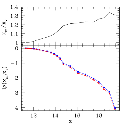
Figure 4: (bottom) Evolution of the ionized fractions: mass-weighted, $x_{m}$, (blue, solid, squares) and volume-weighted, $x_{v}$, (red, dashed, triangles); and (top) their ratio, vs. redshift $z$.

Our code is parallelized for SMP machines using OpenMP and runs highly efficiently, fully utilizing all processors assuming there is sufficient memory for all threads. This particular simulation took 2 weeks of computing time on a Compaq machine with 32 alpha processors running at 733 MHz. At $203^{3}$ resolution the code requires $\sim 0.4$ GB of RAM per computing thread (12 GB total for 32 threads). The code also readily runs on a single- or dual-processor workstation. On a single processor PC this simulation requires 680 MB of RAM and would take about 2 months of computing time on a current 64-bit Opteron workstation.

3 Results

3.1 Globally-Averaged Quantities

We start our analysis of the results by deriving from our simulation a number of globally-averaged characteristics of the reionization process. While such averaged quantities carry no direct information about the geometry of reionization, they do have important observational and theoretical implications.

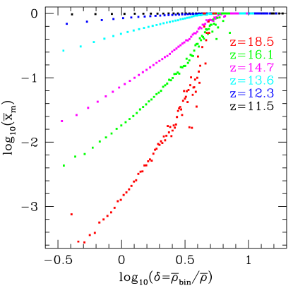
Figure 5: A histogram of $\bar{\rho}_{\rm bin}/\bar{\rho}$, the average ionized mass fraction of the computational cells with a given overdensity, for several redshifts, as indicated (bottom to top from the highest to the lowest redshift, labeled also by color).

3.1.1 Mass- and volume weighted ionization fractions

In our simulations the first ionizing sources form around $z\sim 21$ and final overlap (defined by less than 1% neutral fraction remaining) is reached by $z\sim 11.3$. The first sources are highly clustered, in accordance with the Gaussian statistics of high density peaks within which these first halos form, and are surrounded by regions with density well above the cosmic mean. In Figure (4) we show the evolution of mass-weighted ($x_{m}$) and volume-weighted ($x_{v}$) ionized fractions during the course of our simulation. The mass-weighted ionized fraction starts significantly higher, by 30-35%, than the volume-weighted one. The difference between the two steadily decreases thereafter but remains above one throughout the evolution, eventually asymptoting to one when the whole computational volume becomes ionized. The ratio of the two ionized fractions, $x_{m}/x_{v}$, is in fact equal to the average gas density in the ionized regions in units of the mean density of the universe:

$$\frac{x_{m}}{x_{v}}=\frac{V_{\rm box}}{M_{\rm box}}\frac{x_{m}M_{\rm box}}{x_{v}V_{\rm box}}=\frac{1}{\bar{\rho}}\frac{M_{\rm ionized}}{V_{\rm ionized}}$$ (3)

This is a manifestation of the predominantly inside-out character of reionization. The high-density regions and local density peaks surrounding the sources are ionized first. The ionization fronts then expand further into both high- and low-density nearby regions, with the material in the large voids ionized last. This point is further illustrated in Figure 5, where we show the histogram of the mean mass ionized fraction of all computational cells in a given density bin (in units of the mean density) at several redshifts, as indicated, covering the full range of interest. The highest-density cells are almost instantly ionized and remain ionized throughout the simulation, while the lower-density cells take progressively longer to become ionized. Higher-density cells are on average always more ionized than lower-density ones. Naturally, close to overlap the average density of the ionized regions approaches the global mean density, and both high- and low-density cells become mostly ionized.

Figure 6: (left) Time-integrated number of recombinations per total atom in our simulation volume, $\bar{n}_{\rm rec}$, vs. redshift. (right) Evolution of the effective clumping factor, $C_{\rm eff}=\langle n_{HII}^{2}\rangle/\langle n_{HII}\rangle^{2}$, of the ionized gas.

3.1.2 Average number of recombinations and effective gas clumping factor

In Figure (6, left) we plot the time-integrated number of recombinations per total atom in our simulation volume, $\bar{n}_{\rm rec}$, vs. redshift. This number of recombinations starts low, since even within the denser regions which surround each source the recombination time is relatively long. Around $z\sim 14$ $\bar{n}_{\rm rec}$ quickly rises, eventually reaching $\sim 0.6$ at overlap – i.e. each atom in the computational volume experienced on average 0.6 recombinations. This rise is due to the longer time that atoms have had to recombine, but also due to the evolution of cosmological structure, which leads to a clumpier gas distribution, thus increasing the recombination rate. This increase occurs even though $\bar{n}_{\rm rec}$ is continuously “diluted” by averaging the total number of recombinations over ever larger ionized fraction.

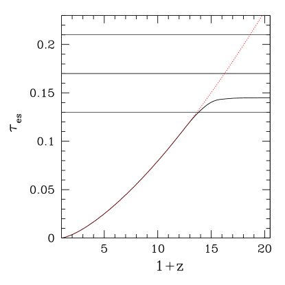
Figure 7: Integrated optical depth due to electron scattering $\tau_{\rm es}$ vs. redshift $z$ (solid). Top (dotted) curve shows the optical depth produced assuming complete ionization out to the corresponding redshift. Horizontal lines indicate the best-fit and $1-\sigma$ uncertainties of the first-year WMAP result, $\tau_{\rm es}=0.17\pm 0.04$.

The number of recombinations per atom in our simulation is somewhat low due to the relatively coarse resolution of our radiative transfer grid, which effectively filters the small-scale fluctuations. In Figure (6, right) we plot the effective gas clumping factor in the ionized regions, defined the usual way, $C_{\rm eff}=\langle n_{HII}^{2}\rangle/\langle n_{HII}\rangle^{2}$. Similarly to $\bar{n}_{\rm rec}$, to which it is related, the effective gas clumping starts quite low, and grows quickly after $z\sim 15$ as H II regions start to encompass both high- and low-density regions and cosmological structure formation progresses, reaching 1.25 towards the end of our simulation. The mean clumping factor is always close to one due to the large scales our simulation is probing, at which the density fluctuations are relatively small. The effect of this on reionization should be studied further, by running higher-resolution simulations and/or including additional gas clumping at sub-grid scales.

3.1.3 Thomson optical depth

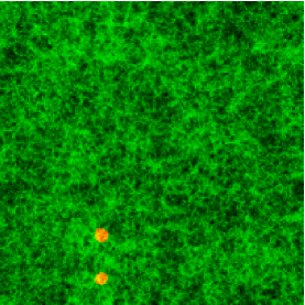
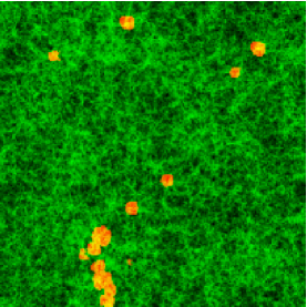
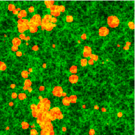
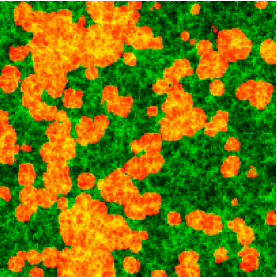
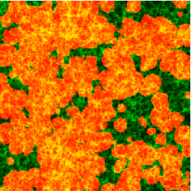
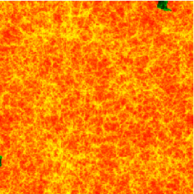
Figure 8: Slices through the simulation volume at redshifts $z=18.5,16.1,14.5,13.6$, $12.6$ and $11.3$. Shown are the density field (green in neutral regions, yellow in ionized regions) and the H II regions (red). See $\tt www.cita.utoronto.ca/\!\sim\!iliev/research.html$ for animations of this and other cuts through our simulation volume. For reference the simulation box angular size on the sky at this redshift range is from $\sim 45^{\prime}$ (at $z=18.5$) to $\sim 49^{\prime}$ (at $z=11.3$).

For any given reionization history, the mean optical depth along a line-of-sight between an observer at $z=0$ and a redshift $z$ due to Thomson scattering by free electrons in the post-recombination universe is an integrated quantity, given by

$$\tau_{\rm es}(z)=c\sigma_{T}\int^{0}_{z}dz^{\prime}n_{e}(z^{\prime})\frac{dt}{dz^{\prime}},$$ (4)

where $\sigma_{T}=6.65\times 10^{-25}\rm cm^{2}$ is the Thomson scattering cross-section, $c$ is the speed of light, and $n_{e}(z)$ is the mean number density of free electrons at redshift $z$, given by

$$n_{e}(z)=n_{H}^{0}(1+z)^{3}x_{m}(z),$$ (5)

where $n_{H}^{0}$ is the mean number density of hydrogen at present. We ignore the presence of helium here, which has only a small effect on the total electron scattering optical depth. For comparison with the value of $\tau_{\rm es}$ between us and the surface of last scattering inferred from measurements of the polarization of the CMB, we evaluate $\tau_{\rm es}(z)$ at $z=z_{\rm rec}$, the redshift of recombination, integrating over our simulation data.

If we assume that $x_{m}=\rm const$ between us and a given redshift $z$ (e.g. for an IGM fully ionized since overlap $x_{m}=1$) the integral in equation (4) has a closed analytical form (Iliev et al. 2005a)

$$\tau_{\rm es}(z)=\frac{2c\sigma_{T}\Omega_{b}\rho_{\rm crit,0}}{3H_{0}m_{p}\Omega_{0}}x_{m}\left\{[\Omega_{0}(1+z)^{3}+\Omega_{\Lambda}]^{1/2}-1\right\}.$$ (6)

For $x_{m}=1(0)$ for $z\leq z_{\rm ov}$ ($z>z_{\rm ov}$), $\tau_{\rm es}\geq 0.035$ for $z_{\rm ov}\geq 6$, where $z_{\rm ov}$ is the redshift of overlap. We used this analytical expression to evaluate the integrated electron scattering optical depth between the present and the overlap, where our simulation stops. In Figure (7) we show the integrated electron scattering optical depth we obtained. Our derived value, $\tau_{\rm es}=0.145$ is well within the $1-\sigma$ limits from the most probable value found from the first year WMAP data.

3.2 The geometry of reionization

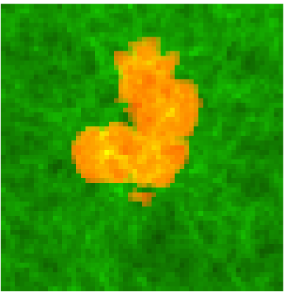
Figure 9: Zoomed-in image of an early H II regions at redshift $z=16.76$. We used a higher-resolution ($406^{3}$ grid) version of the same simulation to show more detail. Note the complex, non-spherical shape. It is caused partly by the slower I-front propagation along the filaments and sheets of the cosmic web and partly by merging several H II regions.

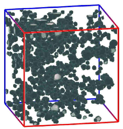
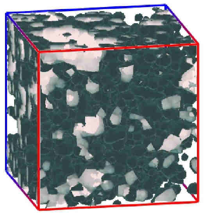
Figure 10: Volume rendering of the H II regions at redshifts $z=14.74$ (left) and $z=13.62$ (right). The 50% ionization iso-surfaces are shown in dark color, while the light color volume-renders the ionized gas density. (Images produced using the IFRIT visualization package of N. Gnedin)

We start our discussion of the large-scale geometry of reionization by examining a sequence of cuts through our simulation box, shown in Figure 8. The first H II regions appear in our simulation quite early, at $z\sim 21.5$ and they expand fast to a few comoving Mpc by redshift $z\sim 18$. These first H II regions are roughly spherical, although close examination reveals that they have more complex shapes, partly dictated by the slower I-front propagation along the filaments and sheets of the cosmic web and partly by merging several H II regions. A zoomed-in sample is shown in Fig. 9). However, filaments cover only a very small fraction of each source’s sky, and this fact, in addition to the relatively coarsely-resolved density field, results in a roughly spherical geometry of the isolated H II regions. These first ionizing sources are highly clustered, and hence the H II regions do not stay isolated for long and quickly merge together into larger and quite-irregularly shaped ionized regions. Hence, early-on (redshifts $z=16.1$ and $z=14.5$ in Figure 8) the geometry of reionization is dominated by the local source clustering at the highest density peaks and along dense filaments. As reionization progresses ($z\sim 13-14$) many more sources form and they become less clustered. By then both the volume and mass ionized fractions are about a half and there are 1-3 large regions, of sizes tens of Mpc, which resulted from the mergers of a number of smaller ionized bubbles. This creates a local overlap, while at the same time similar-size neutral H I regions exist as well. Thereafter the number of ionizing sources in the box continues to grow strongly as they become more common, reaching tens of thousands in our volume. The large H II regions continue to percolate locally, creating ever larger ionized zones with quite complex shapes and structures. At the same time there are a number of smaller H II regions appearing around newly-formed sources. Eventually the whole box becomes ionized at $z\sim 11.3$. In Figure 10 we show a 3D volume rendering of the H II regions at redshifts $z=14.74$ and $z=13.62$ to give the reader a better sense of their distribution in space and their complex shapes.

3.2.1 Correlation between density and ionization

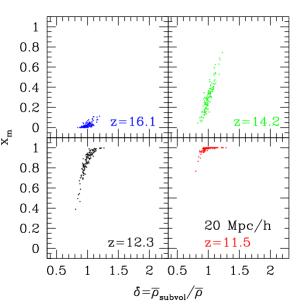
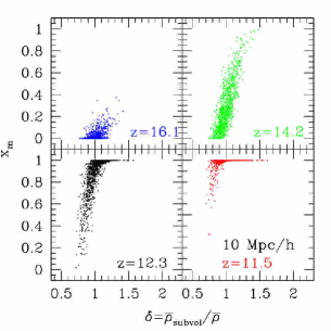
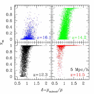
Figure 11: Correlation of the mass-weighted ionized fraction $x_{m}$ in all non-overlapping cubical sub-regions of size $20\,h^{-1}$ Mpc (left), $10\,h^{-1}$ Mpc (middle) and $5\,h^{-1}$ Mpc (right) in our simulation volume with the average density of that region (in units of the mean density of the universe), $\delta=\langle{\rho}\rangle/\bar{\rho}$ at several redshifts, as labeled.

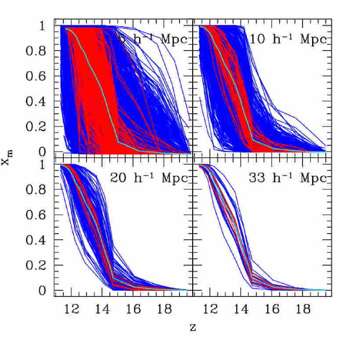
Figure 12: Evolution of the mass-weighted ionized fraction $x_{m}$ (shown in blue) in all non-overlapping cubical sub-regions of sizes $5\,h^{-1}$ Mpc (top left), $10\,h^{-1}$ Mpc (top right), $20\,h^{-1}$ Mpc (bottom left) and $33\,h^{-1}$ Mpc (bottom right), and the sub-group of these which are at the mean density (red). Also shown is the global evolution of the mass ionized fraction (cyan) (the same as in Fig. 4). Even for mean-density sub-regions there is large scatter if the regions are smaller than few tens of Mpc. The magnitude of this scatter is $\Delta z\sim 1-1.5$ for the 20 Mpc regions, $\Delta z\mathrel{\hbox{\hbox to0.0pt{\hbox{\lower 4.0pt\hbox{$\sim$}}\hss}\hbox{$>$}}}2$ for the 10 Mpc regions and $\Delta z\sim 3-4.5$ for the 5 Mpc ones.

Figure 13: (left) The variance, $\Delta$ of the 3D power spectra of the neutral gas density (dotted), total density (solid) and ionized gas density (dashed) all normalized to the total, at various redshifts, as labeled. (right) Ratios of the power spectra of the neutral density to the total density, $\Delta_{\rho,\rm HI}/\Delta_{\rho}$, and of the ionized density to the total density, $\Delta_{\rho,\rm HII}/\Delta_{\rho}$.

We found a clear but complicated correlation between the average density of a region in space and its reionization history. This is not unexpected since we have already shown above that denser regions are ionized earlier than the less dense ones. The fact that reionization history of a region depends on the mean density of that region has been previously pointed out in (Ciardi et al. 2003), where the reionization histories of an overdense region of size $10\,h^{-1}$ Mpc and a mean-density one of size $20\,h^{-1}$ Mpc have been compared. The correlation we find has significant scatter and is strongly dependent on the redshift and the size of the regions considered. In Figure 11 we show a scatter plot at several different redshifts of the ionized mass fraction of all non-overlapping cubical sub-regions of sizes $5\,h^{-1}$ Mpc, $10\,h^{-1}$ Mpc and $20\,h^{-1}$ Mpc vs. their respective average density (in units of the mean density). The overdensity-ionized fraction correlation is most clear for the larger, $20\,h^{-1}$ Mpc regions, albeit still with significant scatter. More importantly, the slope of the mean correlation gets steeper with time, and its shape changes as well. The most overdense regions of that size become completely ionized by redshift $z=13.6$ and drop from the correlation, and by $z=11.5$ all sub-regions with mean density or above do the same.

For the smaller, $10\,h^{-1}$ Mpc sub-regions the range of densities is much larger and the correlation still exists but with even larger scatter. Again we notice that the mean correlation grows steeper in time, to the point of almost disappearing at $z=11.5$ close to overlap. For the small, $5\,h^{-1}$ Mpc sub-regions these trends become even more pronounced, with a huge scatter and almost vertical (i.e. no correlation) mean relation starting from $z\sim 12$.

These results clearly show that no simple relation between the mean density of a region in space and its reionization history exists. The two quantities are clearly correlated, except for small regions at late times, but with significant scatter and a mean behavior that depends on redshift and the region’s size. For smaller regions at late times the correlation essentially disappears, with the densest regions completely ionized and the less dense regions at all different ionization stages independent of their mean density.

This complex behavior of the sub-region reionization histories is further illustrated in Figure 12, where we show the evolution of the mass-weighted ionized fractions, $x_{m}$ for all sub-regions of the same size (for sizes $5\,h^{-1}$ Mpc, $10\,h^{-1}$ Mpc, $20\,h^{-1}$ Mpc and $33\,h^{-1}$ Mpc, as labeled), as well as of the sub-group of these which are within 1% of the mean density of the universe. Also indicated is the evolution of the mass ionized fraction for the total simulation volume. The evolutionary tracks vary greatly for the small, $5$ and $10\,h^{-1}$ Mpc regions, with scatter in redshift at a given ionized fraction $x_{m}$ of up to $\Delta z\sim 5$. This scatter is somewhat smaller, $\Delta z\sim 1-1.5$, but is still significant for the larger, $20\,h^{-1}$ Mpc sub-regions and essentially disappears for the $33\,h^{-1}$ Mpc mean-density sub-regions, although there is still some scatter for over- and under-dense regions. The global ionized fraction evolution is reasonably well-represented only by the mean-density $33\,h^{-1}$ Mpc and $20\,h^{-1}$ Mpc sub-regions.

There are a couple of reasons for this scatter and the complex behavior of the density-ionized fraction relation. The mean density of a region in space is only an approximate indicator of both the number of sources inside that region and of the level of the density fluctuations (which dictate the local recombination rate). Additionally, the radiative input is non-local, i.e. sources outside a given region can, and do, influence its evolution. Both of these effects are much stronger for smaller regions and practically disappear for the $33\,h^{-1}$ Mpc regions since these are large enough to reproduce the mean behaviour of the universe at large. E.g. external sources matter less for large regions since at large distances there is sufficient optical depth to minimize their effect and limit it to the outer edges of the region. This clearly demonstrates that small-box reionization simulations are subject to a large cosmic variance, result in a range of different reionization histories, and cannot be used to determine precisely the redshift of overlap. Simulation boxes of at least a few tens of Mpc are required for any precision and simulations with box sizes smaller than $\sim 10$ Mpc contain essentially no information about the redshift of overlap.

3.2.2 Power spectra of the H I and H II regions

The 3D power spectrum $\Delta(k)$ of a density field $\delta({\bf x})$ (in units of the mean) is given by

$$\Delta^{2}(k)\equiv\frac{k^{3}}{2\pi^{2}V}\sigma_{k}^{2}=\frac{k^{3}}{2\pi^{2}V}\int\delta^{2}({\bf x})e^{-i{\bf k}\cdot{\bf x}}d^{3}x$$

$$=\frac{k^{3}}{2\pi^{2}V}\langle\delta(k)\delta(-k)\rangle,$$ (7)

where $V=L^{3}$ is the associated volume and ${\bf k}=(2\pi/L){\bf n}$ is the wavenumber, where ${\bf n}$ is an integer vector. If in equation (7) we identify the field $\delta({\bf x})$ with the field of the ionized gas density fluctuations, given by $x\delta({\bf x})$, or the neutral gas density fluctuations, given by $(1-x)\delta({\bf x})$, we obtain the power spectra corresponding to these fields. In Figure 13 (left) we plot the results for the 3D power spectra of density fluctuations, $\Delta_{\rho}$ (solid), neutral gas density fluctuations, $\Delta_{\rho,\rm HI}$ (dotted), and ionized gas density fluctuations, $\Delta_{\rho,\rm HII}$ (dashed) at redshifts $z=20.3,17.5,16.1,14.7,13.6,12.9,12.3,11.9,$ and 11.3, as indicated, which cover the complete range of our simulations. Early-on most of the gas is neutral, and thus the neutral gas density power spectrum closely follows the total gas density one. As reionization progresses, its intrinsic patchiness causes both the neutral and ionized gas density fluctuations to rise well above the ones of the total gas density for wavenumbers around and below the wavenumber corresponding to the typical patch size at that time. The wavenumbers for which the fluctuations are strongly increased are roughly independent of redshift, $k\mathrel{\hbox{\hbox to0.0pt{\hbox{\lower 4.0pt\hbox{$\sim$}}\hss}\hbox{$<$}}}{\rm few}\,\rm hMpc^{-1}$ (i.e. scales larger than few comoving Mpc). This strong boost in power, by a (scale-dependent) factor of up to $\sim 3$ (we show the ratios of $\Delta_{\rho,\rm HI}$ and $\Delta_{\rho,\rm HII}$ to $\Delta_{\rho}$ in Figure 13, right), remains in effect for the neutral gas density field until $z\sim 12$, and for the ionized gas density field until the overlap epoch, after which the ionized and total density fluctuations power spectra of course coincide. At late times the neutral gas density fluctuations decrease well below the total density ones due to the very small remaining neutral fraction.

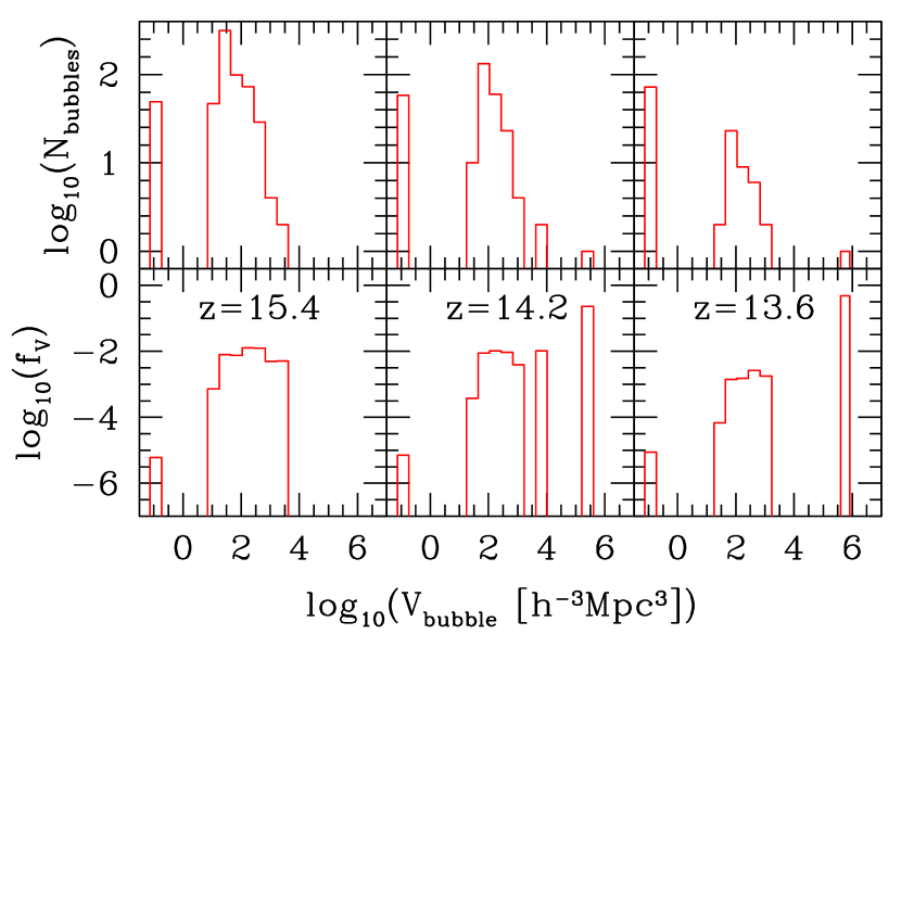
Figure 14: Size distribution of ionized regions: histograms vs. bubble volume, $V_{\rm bubble}$ of (top) Number of H II bubbles of that size, and (bottom) volume-filling factor, $f_{V}$, of the H II bubbles of that size.

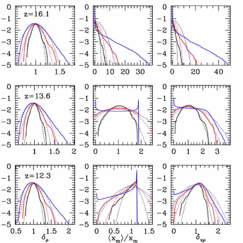
Figure 15: Non-Gaussianity of reionization: PDF distribution functions of (left column) the density in units of the mean density, $\delta_{\rho}=\langle\rho\rangle/\bar{\rho}$, (middle column) the mass ionized fraction in units of the mean one, $\langle x_{m}\rangle/x_{m}$, and (right column) the ionized density in units of the mean ionized density, $\delta_{x\rho}=\delta_{\rho}\langle x_{m}\rangle/x_{m}=\langle x\rho\rangle/(x_{m}\bar{\rho})$, at redshifts $z=16.1$ (top panels), $z=13.6$ (middle panels), $z=12.3$ (bottom panels), for cubical regions of sizes $20\,h^{-1}Mpc$ (black solid), $10\,h^{-1}Mpc$ (red solid), and $5\,h^{-1}Mpc$ (blue solid). Also indicated are the Gaussian distributions with the same mean values and standard deviations (dotted, corresponding colors).

Figure 16: Standard deviations (rms fluctuations) of the ionized gas density, $\sigma_{x\rho}$ (top, thick lines) and of the total gas density, $\sigma_{\rho}$ (bottom, thin lines) vs. scale at redshifts $z=16.1$ (solid), $z=13.6$ (dashed) and $z=12.3$ (dotted).

3.3 Size distributions of the H II regions

In order to find the individual ionized regions and their volumes, we employed a friends-of-friends (FOF)-type algorithm, as follows. Two neighboring cells are considered “friends” and linked together if both of their ionized fractions are larger than 0.5. Ionized cells are thus grouped together into separate, topologically-connected bubbles. We use the “equivalence class” method from Numerical Recipes (Press et al. 1992) to determine the groups. This way we created catalogues of H II bubbles and were able to calculate their numbers in our volume and follow their “merger history” in a way similar to the one used for finding halos in N-body simulations. It should be noted, however, that although there are many similarities between the two cases, as well as an obvious intimate connection between the source halos and the H II regions they create, there are also some important differences between the two distributions and merger histories. For example, due to the nature of the gravitational interaction, halos always grow in mass, while the ionized bubbles can also shrink if the total ionizing emissivity in the bubble decreases, due to, e.g., the death of one or more source. (This does not occur in the current simulations, but is expected to happen when small sources fall below the ionized gas Jeans mass. However, these are below our current resolution and thus not considered here). Clustering and other properties of these two catalogues could be expected to be quite different, as well. Thus, one should exercise care when making such parallels.

Our results are shown in Figure 14. The total number of bubbles starts low, at only a few, around the first sources that form in our box at $z\sim 21$. It then grows as the number of sources grows, reaching a high of $\sim 600$ around $z\sim 14-15$, still well short of the total number of ionizing sources present then (1,500-8,000), since multiple bubbles overlap even at these early times. Most H II regions have a volume of a few tens up to $\sim 10^{3}\,\rm(h^{-1}Mpc)^{3}$ at that time. The first large bubbles, with volumes $>10^{4}\,\rm(h^{-1}Mpc)^{3}$, emerge in our simulation around $z\sim 15$. Thereafter, the total number of bubbles steadily declines, and their sizes grow as they merge, mostly with the largest bubbles present. By redshift $z\sim 14.2$, there are three H II regions larger than $10^{4}\,\rm(h^{-1}Mpc)^{3}$, and each of these occupies a few per cent or more of our simulation volume. By $z\sim 13.6$ these percolate into one huge bubble which occupies about half of the total volume. There is still a large number of smaller H II regions with volumes $\mathrel{\hbox{\hbox to0.0pt{\hbox{\lower 4.0pt\hbox{$\sim$}}\hss}\hbox{$<$}}}10^{3}\,\rm(h^{-1}Mpc)^{3}$. By redshift $z\sim 11.5$ (close to overlap) percolation is complete and only a single connected bubble remains.

In summary, our results indicate that once the ionized fraction surpasses $\sim 10\%$ there are two distinct populations of H II regions in size, a large number of medium-sized, $\sim 10^{3}\,h^{-1}\rm Mpc^{3}$ volumes, or $\sim 10\,h^{-1}$ Mpc size bubbles and a few, rare, very large bubbles with volumes $>10^{4}\rm(h^{-1}Mpc)^{3}$, or sizes of tens of Mpc. (There is also a population of small, one-cell H II regions, where the I-front from an ionizing source becomes temporarily trapped by its own cell.) In terms of ionized volume, the few large bubbles dominate the total by far, while the mid-size regions take only a few percent of the total. Should this behaviour prove robust, this would have important consequences for the observability of reionization. The large bubbles would facilitate the direct detection of the ionization sources through, e.g., Lyman-$\alpha$ emitter number counts and clustering. Such studies would be much more difficult with the sources in the smaller H II regions since the source fluxes from these would be damped by nearby neutral hydrogen. Such very large-scale individual features would also be the easiest objects to detect with the next generation observations in 21-cm line of hydrogen. On the other hand, the smaller, but numerous ionized bubbles (and neutral patches) create the large boost of the fluctuations at intermediate scales (1’-10’) of either the neutral or the ionized gas densities which we discussed above, demonstrated also by the power spectra in Fig. 13. This creates a peak in the fluctuations at these scales, which would be the largest statistical signal from reionization, important for the upcoming and planned 21-cm and kSZ effect observations.

3.4 Beyond the power spectrum: the non-Gaussian nature of reionization

The power spectra discussed above provide an important but very limited description of the statistics of reionization. Similar to the statistics of cosmological density fields, probability distribution functions (PDF) are required to provide more detailed description of the reionization statistics. In Figure 15 we show the PDFs ($p(y)dy$, where $\int p(y)dy=1$) of the density field (left column), mass-weighted ionized fraction field (middle column), and the ionized mass field, all in units of their respective means, for (cubical) regions of size $20\,h^{-1}$ Mpc, $10\,h^{-1}$ Mpc, and $5\,h^{-1}$ Mpc at redshifts $z=16.1$ (top), $z=13.6$ (middle), and $z=12.3$ (bottom). We also show the corresponding Gaussian distributions with the same means and standard deviations. As expected, the total density PDFs are Gaussian on large, linear scales, and increasingly non-Gaussian at the smaller scales. At high densities there are long non-Gaussian tails due to non-linear structure formation.

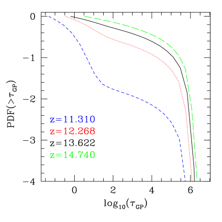
Figure 17: Gunn-Peterson optical depths: (left) Probability distribution of cell-by-cell Gunn-Peterson optical depths larger than a given value $\tau_{GP}$ at redshifts $z=14.740$ (long-dashed), $z=13.622$ (solid), $z=12.268$ (dotted) and $z=11.310$ (short-dashed). (right) Median value, ${\tau}_{\rm GP,median}$ (solid), mean value, $\bar{\tau}_{\rm GP}$ (dotted), and standard deviation, $\sigma_{\tau_{\rm GP}}$ (dashed), of the $\tau_{\rm GP}$ values.

In contrast, the mass ionized fraction distributions (middle) are generally strongly non-Gaussian. Early-on the distributions are strongly-peaked at $\langle x_{m}\rangle/x_{m}\sim 0$, especially for small-size regions since the vast majority of them are still neutral. However, at smaller scales, which are comparable to the H II region’s typical sizes at that time, there is a long tail of highly-ionized regions well above the corresponding Gaussian. At $z=13.6$ we notice a new feature, whereby the distribution inverts for scales below the characteristic size of the H II regions, since in this case the sub-regions probed typically are either close to fully-ionized or to fully-neutral. At scales larger than the typical bubble size this PDF is approximately Gaussian, but significantly wider than the corresponding density field PDF distribution (see also Figure 16) and with a sharp cutoff at the maximum ionization fraction for a region of a given size, $\langle x_{m}\rangle_{\rm max}/x_{m}(z)$, where $\langle x_{m}\rangle_{\rm max}=1$ except at the largest scale (i.e. some regions of these sizes are fully-ionized). At late times the PDFs of the ionized fraction become once again strongly non-Gaussian at all scales, with a long tail at small values of $\langle x_{m}\rangle$ and a sharp cutoff at $1/x_{m}(z)$.

Finally, we show the ionized gas density PDF in the right column of panels. Since the ionized density field is a convolution of the (approximately) Gaussian density field and strongly non-Gaussian mass-weighted ionized fraction field, the resulting PDF exhibits features from both and generally remains significantly non-Gaussian. At high redshifts the PDFs generally follow the ionized fraction PDFs, but with some additional boost of the high-values tail due to the strong correlation between high ionization and high density (inside-out reionization) at these redshifts. At intermediate redshifts the PDF shapes are roughly Gaussian at large scales, but wider than the corresponding density PDFs (see also Figure 16), and quite non-Gaussian at small scales. At late times the PDF shapes remain significantly non-Gaussian at all scales. The maxima of the distributions are offset towards the larger values compared to the mean distribution values and the decreases of the probabilities at smaller values of $\delta_{x\rho}$ are less steep than a Gaussian due to the correlation between the low-density voids and low ionization levels discussed above.

In Figure 16 we show the standard deviations (i.e. rms fluctuations) of the ionized density field, $\sigma_{x\rho}$, and the total density field, $\sigma_{\rho}$, vs. scale $L$. As noted above, the ionized density distributions are considerably wider than the corresponding total density distributions. They also vary significantly more with redshift, and decrease as time goes by, unlike the total density fluctuations which increase with time as cosmological structures develop.

3.5 Gunn-Peterson optical depths

The observability of high-redshift Ly-$\alpha$ sources ($\lambda_{\alpha}=1216$Å) depends upon the gas ionization levels along the line-of-sight towards the observer. The Gunn-Peterson (GP) optical depth of the IGM at redshift $z$ is given by

$$\tau_{\rm GP}=\sigma(\nu)n_{\rm HI}(z)(1+z)\left|\frac{dt}{dz}\right|,$$ (8)

where $n_{\rm HI}(z)$ is the neutral hydrogen density, $\sigma(\nu)=\frac{\pi e^{2}}{m_{e}}f\delta(\nu-\nu_{\alpha})$ is the absorption cross-section ($e$ and $m_{e}$ are the charge and mass of the electron, and $f=0.416$ is the oscillator strength of the 2p to 1s energy level transition), and for flat $\Lambda$CDM at high redshift, which is the relevant regime here,

$$\left|\frac{dt}{dz}\right|=\frac{1}{H_{0}\Omega_{0}^{1/2}(1+z)^{5/2}}.$$ (9)

Numerically, the GP optical depth at a point is then given by

$$\tau_{\rm GP}=1.146\times 10^{11}\,n_{\rm HI}(z)(\rm cm^{-3})(1+z)^{-3/2}$$ (10)

The probability distribution of this optical depth provides a rough idea about the observability of the sources in our simulation. In Figure 17 (left) we show the probability distribution for a cell to have $\tau_{\rm GP}$ larger than a given value. We see that only quite close to overlap (after $z\sim 12$ for this particular simulation) the majority of the cells become optically-thin. In Figure 17 (right) we plot the median value, ${\tau}_{\rm GP,median}$, mean value, $\bar{\tau}_{\rm GP}$, and standard deviation, $\sigma_{\rm GP}$ for all cells vs. redshift. Close to overlap all three drop significantly from their peaks, but while the mean value and scatter remain high, the median optical depth drops (marginally) below one. This behaviour reflects the fact that while the majority of cells are highly ionized close to overlap, there exists a minority of cells which are still highly optically-thick, which results in a high mean value and scatter for the PDF of the optical depths. Apparently, the epoch of overlap has a significant, detectable Gunn-Peterson optical depth throughout a substantial fraction of the volume. This is expected since the neutral fraction in the ionized zones just prior to their overlap is high enough, even though it is quite small, to make $\tau_{\rm GP}\mathrel{\hbox{\hbox to0.0pt{\hbox{\lower 4.0pt\hbox{$\sim$}}\hss}\hbox{$>$}}}1$ and it is necessary to pass the epoch of overlap before the UV background rises significantly due to the appearance of more distant sources (Shapiro et al. 1987). More precise predictions for the observability of these emitters would require taking into account the positions of the sources and the detailed geometry of the ionized bubbles around them, which goes beyond the scope of the current paper and will be explored in a follow-up work.

4 Summary and Conclusions

We have presented the first large-scale radiative transfer simulation of the reionization of the universe. The total electron-scattering optical depth produced by our simulation agrees well with the results on CMB polarization from the first-year WMAP data, but the final overlap occurs at $z\sim 11$, somewhat too early to clearly agree with the current observations of high-z QSOs and galaxies, which point to reionization ending around $z=6-7$. However, we note that there are several effects which we do not include here which are expected to extend reionization without destroying the agreement with the WMAP results on the optical depth. These effects include small-scale (here sub-grid) gas clumping and lower ionizing efficiency of the sources, among others (Iliev et al. 2005a). We are currently working on studying these effects in more detail with further simulations.

For a fixed distribution of sources the I-fronts escape from the high-density gas surrounding the sources and propagate faster into the lower-density gas in voids. This led to predictions in earlier work that reionization proceeded “outside-in”, instead, with the preferential ionization of the lower-density regions (e.g. Gnedin 2000). We have seen some such behaviour in the toy test runs we performed as a simple application in Mellema et al. (2006a). However, the full reionization simulation we have presented here points to the opposite conclusion. We demonstrated that in our simulation the process is “inside-out”, i.e. with the high-density regions ionized earlier on average, and the large voids reionized last. The main reason for this is that the character of reionization is dictated by the interplay between H II region expansion and evolving structure formation. The ionizing sources at high redshifts formed at the highest-density, rare peaks of the density field. As the cosmological structure formation progresses, more and more new sources form inside the density peaks, as these collapse. Thus, even though the I-fronts due to the earliest source clusters might escape into nearby voids and ionize them quickly, the numerous newly-formed sources ensure that on average there is always more mass ionized than volume. Earlier simulations which predicted “outside-in” reionization employed much smaller boxes, which resulted in faster reionization and less evolution in the source population in that time period.

This inside-out nature of reionization leads to an increased ionizing photon consumption since denser and clumpier gas has shorter recombination times, resulting in multiple recombinations per atom. In our particular simulation approximately 1.6 ionizing photons per atom were eventually required for completing the process. Our conclusions are not affected by the relatively coarse resolution of the simulation presented here, with cell size $\sim 0.5\,h^{-1}$ Mpc, which significantly filters the density fluctuations. We have now also run a simulation with the same underlying density field and sources, but with higher radiative transfer grid resolution ($406^{3}$ cells) (Mellema et al. 2006b), as well as multiple simulations with smaller box size ($35\,h^{-1}$ Mpc), and thus higher spatial resolution (Iliev et al. 2006). Increased spatial resolution and the corresponding higher density contrasts emphasizes the inside-out nature of reionization even more and only strengthtens our current conclusions. In turn, such increased ionizing photon consumption would require fairly efficient production of ionizing photons at high-z, either due to massive, hot stars, high efficiency of star formation, high escape fractions, or a combination of all these.

Our current simulation does not include the effects of mechanical feedback (e.g. from supernovae) which can disrupt the smaller sources and modify their star formation rates. Currenly we also do not include the radiative input from ionizing sources with halo masses smaller than $2.5\times 10^{9}\,M_{\odot}$, which are below the resolution of our N-body simulation. Hence, our source population should be considered a low limit to the realistic one. These effects would be studied in a subsequent work (Iliev et al. 2006).

The scale of our simulation has allowed us for the first time to study numerically the large-scale geometry and statistics of reionization. We derived the correlation between the density of a region and its ionization state. We showed that the relation is complex and its mean and dispersion are significantly redshift- and scale-dependent. At late times and small scales the correlation essentially disappears. Furthermore, we demonstrated that the reionization history of sub-regions exhibits significant scatter at small scales and provides good description of the mean behaviour only at large scales, above 20-30 $h^{-1}$ Mpc.

The patchiness of reionization results in a significant increase of both the neutral- and ionized-gas density fluctuations, with important implications for statistical observations of reionization at, e.g., the 21-cm line of neutral hydrogen (Mellema et al. 2006b) and small-scale CMB anisotropies. The power spectra of ionized and neutral density fluctuations at wavenumbers $k\mathrel{\hbox{\hbox to0.0pt{\hbox{\lower 4.0pt\hbox{$\sim$}}\hss}\hbox{$>$}}}1\,\rm h\,Mpc^{-1}$ are boosted by up to factors of $\sim 2-3$ compared to the fluctuations of the total gas density. This roughly translates to a stronger fluctuation signal at arcminute and larger scales.

We derived the size distributions of the H II regions in our simulations in both number counts and volume filling factors. We found two populations of bubbles, one with a large numbers of medium-sized ($\sim 10$ Mpc) and one with a few, rare and very large bubbles of size tens of Mpc. The first population provides most of the statistical fluctuations at arcminute scales discussed above, while the large ones should be the most prominent and most easily-detectable features of reionization. We also derived the distribution of Gunn-Peterson optical depths in our simulation volume as a first step to more detailed predictions for the observations of Ly-alpha emitters at high redshift by current and upcoming large surveys.

Finally, we demonstrated and for the first time quantified the non-Gaussian nature of the reionization statistics. The probability distribution functions for both the ionized mass fraction and the ionized mass are generally strongly non-Gaussian on all scales and at all times, especially at the beginning and end of reionization. At scales below the typical scales for the H II regions the distribution even inverts, with the highest probability for a region to be either highly-neutral or highly-ionized. This is a feature of our reionization model, where no sources vary strongly in luminosity over time (or die). This is justified for our ionizing sources, which are relatively large galaxies above the ionized-gas Jeans mass, whose formation cannot, therefore, be easily suppressed. We will study the effects of the presence of smaller ionizing sources and more realistic source behaviour in a follow-up work.

References

- Abel et al. (1999) Abel T., Norman M. L., Madau P., 1999, Astrophys. J. , 523, 66
- Barkana & Loeb (2004) Barkana R., Loeb A., 2004, Astrophys. J. , 609, 474
- Bolton et al. (2004) Bolton J., Meiksin A., White M., 2004, Mon. Not. R. Astron. Soc. , 348, L43
- Cen (2002) Cen R., 2002, Astrophys. J. Suppl., 141, 211
- Cen (2005) —, 2005, ArXiv Astrophysics e-prints (astro-ph/0507014)
- Ciardi et al. (2000) Ciardi B., Ferrara A., Governato F., Jenkins A., 2000, Mon. Not. R. Astron. Soc. , 314, 611
- Ciardi et al. (2003) Ciardi B., Stoehr F., White S. D. M., 2003, Mon. Not. R. Astron. Soc. , 343, 1101
- Fan et al. (2002) Fan X., Narayanan V. K., Strauss M. A., White R. L., Becker R. H., Pentericci L., Rix H.-W., 2002, Astron. J. , 123, 1247
- Furlanetto & Oh (2005) Furlanetto S. R., Oh S. P., 2005, Mon. Not. R. Astron. Soc. , 363, 1031
- Furlanetto et al. (2004) Furlanetto S. R., Zaldarriaga M., Hernquist L., 2004, Astrophys. J. , 613, 1
- Gnedin (2000) Gnedin N. Y., 2000, Astrophys. J. , 535, 530
- Gnedin & Abel (2001) Gnedin N. Y., Abel T., 2001, New Astronomy, 6, 437
- Haiman & Holder (2003) Haiman Z., Holder G. P., 2003, Astrophys. J. , 595, 1
- Hayes & Norman (2003) Hayes J. C., Norman M. L., 2003, Astrophys. J. Suppl., 147, 197
- Iliev et al. (2006) Iliev I. T., Mellema G., Shapiro P. R., Pen U. L., 2006, in preparation
- Iliev et al. (2005a) Iliev I. T., Scannapieco E., Shapiro P. R., 2005a, Astrophys. J. , 624, 491
- Iliev et al. (2005b) Iliev I. T., Shapiro P. R., Raga A. C., 2005b, Mon. Not. R. Astron. Soc. , 361, 405
- Iliev et al. (2005c) Iliev I. T., Shapiro P. R., Scannapieco E., Mellema G., Alvarez M., Raga A. C., Pen U.-L., 2005c, in IAU Colloq. 199: Probing Galaxies through Quasar Absorption Lines, pp. 369–374
- Kohler et al. (2005a) Kohler K., Gnedin N. Y., Hamilton A. J. S., 2005a, ArXiv Astrophysics e-prints (astro-ph/0511627)
- Kohler et al. (2005b) Kohler K., Gnedin N. Y., Miralda-Escudé J., Shaver P. A., 2005b, Astrophys. J. , 633, 552
- Lim & Mellema (2003) Lim A. J., Mellema G., 2003, A.&A, 405, 189
- Malhotra & Rhoads (2004) Malhotra S., Rhoads J. E., 2004, Astrophys. J. Letters., 617, L5
- Maselli et al. (2003) Maselli A., Ferrara A., Ciardi B., 2003, Mon. Not. R. Astron. Soc. , 345, 379
- Mellema et al. (2006a) Mellema G., Iliev I. T., Alvarez M. A., Shapiro P. R., 2006a, New Astronomy, 11, 374
- Mellema et al. (2006b) Mellema G., Iliev I. T., Pen U. L., Shapiro P. R., 2006b, submitted to MNRAS (astro-ph/0603518)
- Mellema et al. (1998) Mellema G., Raga A. C., Canto J., Lundqvist P., Balick B., Steffen W., Noriega-Crespo A., 1998, A.&A, 331, 335
- Merz et al. (2005) Merz H., Pen U.-L., Trac H., 2005, New Astronomy, 10, 393
- Nakamoto et al. (2001) Nakamoto T., Umemura M., Susa H., 2001, Mon. Not. R. Astron. Soc. , 321, 593
- Press et al. (1992) Press W. H., Flannery B. P., Teukolsky S. A., Vetterling W. T., 1992, Numerical Recipes: The Art of Scientific Computing, 2nd edn. Cambridge University Press, Cambridge (UK) and New York
- Press & Schechter (1974) Press W. H., Schechter P., 1974, Astrophys. J. , 187, 425
- Razoumov et al. (2002) Razoumov A. O., Norman M. L., Abel T., Scott D., 2002, Astrophys. J. , 572, 695
- Razoumov & Scott (1999) Razoumov A. O., Scott D., 1999, Mon. Not. R. Astron. Soc. , 309, 287
- Reed et al. (2003) Reed D., Gardner J., Quinn T., Stadel J., Fardal M., Lake G., Governato F., 2003, Mon. Not. R. Astron. Soc. , 346, 565
- Santos et al. (2003) Santos M. G., Cooray A., Haiman Z., Knox L., Ma C.-P., 2003, Astrophys. J. , 598, 756
- Seljak & Zaldarriaga (1996) Seljak U., Zaldarriaga M., 1996, Astrophys. J. , 469, 437
- Shapiro & Giroux (1987) Shapiro P. R., Giroux M. L., 1987, Astrophys. J. , 321, L107
- Shapiro et al. (1994) Shapiro P. R., Giroux M. L., Babul A., 1994, Astrophys. J. , 427, 25
- Shapiro et al. (1987) Shapiro P. R., Giroux M. L., Kang H., 1987, in High Redshift and Primeval Galaxies (Proceedings of the Third IAP Workshop), eds. J. Bergeron, D. Kunth, B. Rocca-Volmerange, and J. Tran Thanh Van (France: Editions Frontieres), pp. 501–515
- Shapiro et al. (2004) Shapiro P. R., Iliev I. T., Raga A. C., 2004, Mon. Not. R. Astron. Soc. , 348, 753
- Sheth & Tormen (2002) Sheth R. K., Tormen G., 2002, Mon. Not. R. Astron. Soc. , 329, 61
- Sokasian et al. (2001) Sokasian A., Abel T., Hernquist L. E., 2001, New Astronomy, 6, 359
- Spergel et al. (2003) Spergel D. N., Verde L., Peiris H. V., Komatsu E., Nolta M. R., Bennett C. L., Halpern M., Hinshaw G., Jarosik N., Kogut A., Limon M., Meyer S. S., Page L., Tucker G. S., Weiland J. L., Wollack E., Wright E. L., 2003, Astrophys. J. Suppl., 148, 175
- Stern et al. (2005) Stern D., Yost S. A., Eckart M. E., Harrison F. A., Helfand D. J., Djorgovski S. G., Malhotra S., Rhoads J. E., 2005, Astrophys. J. , 619, 12
- Wyithe & Loeb (2003) Wyithe J. S. B., Loeb A., 2003, Astrophys. J. , 586, 693
- Zhang et al. (2004) Zhang P., Pen U.-L., Trac H., 2004, Mon. Not. R. Astron. Soc. , 355, 451