VLT-ISAAC 3-5 $\mu$m spectroscopy of embedded young low-mass stars. III. Intermediate-mass sources in Vela

Abstract

Aims. We study in this paper the ice composition in the envelope around intermediate-mass class I Young Stellar Objects (YSOs).

Methods. We performed a spectroscopic survey toward five intermediate-mass class I YSOs located in the Southern Vela molecular cloud in the $L$ (2.85–4.0 $\mu$m) and $M$ (4.55–4.8 $\mu$m) bands at resolving powers $\lambda/\Delta\lambda=$ 600-800 up to 10,000, using the Infrared Spectrometer and Array Camera mounted on the Very Large Telescope-ANTU. Lower mass companion objects were observed simultaneously in both bands.

Results. Solid H₂O at 3 $\mu$m is detected in all sources, including the companion objects. CO ice at 4.67 $\mu$m is detected in a few main targets and one companion object. One object (LLN 19) shows little CO ice but strong gas-phase CO ro-vibrational lines in absorption. The CO ice profiles are different from source to source. The amount of water ice and CO ice trapped in a water-rich mantle may correlate with the flux ratio at 12 and 25 $\mu$m. The abundance of H₂O-rich CO likely correlates with that of water ice. A weak feature at 3.54 $\mu$m attributed to solid CH₃OH and a broad feature near 4.62 $\mu$m are observed toward LLN 17, but not toward the other sources. The derived abundances of solid CH₃OH and OCN^- are $\sim$10 $\pm$ 2% and $\sim$1 $\pm$ 0.2% of the H₂O ice abundance respectively. The H₂O optical depths do not show an increase with envelope mass, nor do they show lower values for the companion objects compared with the main protostar. The line-of-sight CO ice abundance does not correlate with the source bolometric luminosity.

Conclusions. Comparison of the solid CO profile toward LLN 17, which shows an extremely broad CO ice feature, and that of its lower mass companion at a few thousand AU, which exhibits a narrow profile, together with the detection of OCN^- toward LLN 17 provide direct evidences for local thermal processing of the ice.

1 Introduction

Dust grains play an important role in the evolution of clouds from protostellar cores to circumstellar disks. Since dust grains are the main source of opacity, they control the thermal balance of clouds. The surfaces of cold grains act as heat sink for highly exothermic reactions to occur (e.g., formation of H₂) or provide sites for atoms and molecules to freeze on. The freeze-out of molecules like CO is found to be important for regulating the gas phase chemistry of other species (e.g., Bergin1997ApJ...486..316B; Bergin2001ApJ...557..209B; Jorgensen2004A&A...416..603J). The frozen atoms and molecules accumulate on top of a refractory core (silicates, carbonaceous compounds) and form an icy mantle or react with other species to synthesize more complex molecules. The relative chemical composition of this ice mantle is well determined after three decades of studies using both ground-based and space-borne telescopes. The core-mantle grain model is supported by spectropolarimetry studies (e.g., Holloway2002MNRAS.336..425H). Solid H₂O, CO, and CO₂ abound in most lines of sight where ices are detected (deGraauw1996A&A...315L.345D). Sometimes, minor species such as CH₄ ($\sim$2%), HCOOH ($\sim$2%), OCN^- ($\sim$0.2–1%) (e.g., vanBroekhuizen2005A&A), and H₂CO (3–6%) are found (e.g., Boogert1998A&A...336..352B ; Keane2001A&A...376..254K; Boogert2004ApJS..154..359B). By contrast, the presence of other minor constituents such as NH₃ is controversial; its abundance relative to water ice is likely less than $\sim$10% (e.g., Ehrenfreund2000ARA&A..38..427E; Dartois2001A&A...365..144D; Dartois2002A&A...394.1057D; Lacy1998ApJ...501L.105L; Taban2003A&A...399..169T). It should be emphasized that most of these studies refer to high mass young stellar objects.

Solid methanol (CH₃OH) is a particular case. It epitomizes the importance of molecular solids in the understanding of the gas phase chemistry. The radiative association of CH${}_{3}^{+}$ and H₂O is an inefficient gas-phase process that yields methanol abundances of $\sim\leavevmode\nobreak\ 10^{-9}$ relative to H₂ while abundances of 10^-7–10^-6 have been found in hot cores (e.g., Blake1987ApJ...315..621B; Sutton1995ApJS...97..455S). The prevalent view is that the high abundance of gas phase methanol come from the release of large amounts of frozen methanol formed on grain surfaces (Charnley1995ApJ...448..232C; vanderTak2000A&A...361..327V; Horn2004ApJ...611..605H). Methanol ice abundance relative to water ice is found to vary from less than 3% w.r.t. water ice in quiescent regions up to 30% around massive protostars (Dartois1999A&A...342L..32D). If all the methanol ice is released in the gas phase, the abundance of methanol in the gas phase with respect to H₂ will amount to 3 $\times$ 10^-7 – 3 $\times$ 10^-6 assuming that the abundance of water ice with respect to H₂ is $\sim$10^-5 (e.g., Whittet2003dge..conf.....W). A similar situation is found for low-mass objects. Chiar1996ApJ...472..665C set a stringent limit of 5% of methanol with respect to water ice for sources located in the Taurus molecular cloud, while Pontoppidan2003A&A...404L..17P found abundant methanol ice (14–25% of water ice) in 4 out of $\simeq$ 40 envelopes around protostars observed with the VLT. Possible formation routes of solid methanol are also disputed. The formation rate of solid methanol by hydrogenation of CO ice in the absence of energy input (i.e. hot atoms, UV or particle irradiation) measured in laboratory experiments remains controversial (e.g., Hiraoka2002ApJ...577..265H; Hiraoka2005ApJ...620..542H; Watanabe2004ApJ...616..638W).

The advent of 8m class telescopes equipped with large format arrays opens up the opportunity to study large samples of low and intermediate-mass sources. We present here the first observations of molecular ice features in the $L$ (2.8–4.1 $\mu$m) and $M$ (4.5–5.1 $\mu$m) bands toward class I intermediate-mass young stellar objects (YSOs) located in the Vela molecular cloud complex. The spectra were obtained in the context of a large programme using the Infrared Spectrometer And Array Camera (ISAAC) mounted at the Very Large Telescope ANTU (VLT-ANTU) of the European Southern Observatory (ESO). Two major absorption features are observable with ground-based telescopes, along with some weak features. The first strong feature is centered around 3.01 $\mu$m ($\sim$ 3300 cm^-1) and is usually attributed to the stretching mode of solid H₂O. The study of the solid-water profile has been used to better explore the ice structure in the water matrix (e.g., Smith1989ApJ...344..413S; Smith1993MNRAS.263..749S; Maldoni1998MNRAS.298..251M). The feature shows a broad excess absorption beyond 3.2 $\mu$m whose origin is still unclear, although scattering by the larger grains (0.1–1 $\mu$m in radius) in the size distribution is the best candidate (Smith1989ApJ...344..413S; Dartois2001A&A...365..144D).

The other important feature is the solid-CO band at 4.67 $\mu$m (2140 cm^-1), whose profile is sensitive to the shape and size of the grains as well as the ice composition and temperature and is therefore a diagnostic of the evolutionary state and thermal history of ices (Sandford1988ApJ...329..498S). As soon as the grain is warmed to $\simeq$ 12–15 K by the luminosity of the object, CO molecules can diffuse into the ice and form new bonds, changing the morphology of the mixture and thus the profile at 4.67 $\mu$m, or they can sublime back to the gas phase (Al-Halabi2004A&A...422..777A; Collings2003ApJ...583.1058C; Givan1997JPhysChem). The mobility of CO and its high abundance in cold icy mantles also explain why it is a key species for surface reactions leading to polyatomic molecules such as CO₂ and CH₃OH (Rodgers2003ApJ...585..355R; Chiar1998ApJ...498..716C; Teixeira1998A&A...330..711T).

The VLT-ISAAC observations are used to constrain the physical and chemical conditions in the envelopes of a sample of intermediate-mass stars. The paper is organized as follows. We present the objects of our sample in Sect. 2 and the observations and data reduction procedures in Sect. 3. The results on the water ice band are described in Sect. 4.1. Evidence for solid CH₃OH is presented in Sect. 4.2. The CO-ice band is presented in Sect. 4.3. A possible correlation between the abundance of CO embedded into a water ice matrix and the IRAS 12 $\mu$m/ 25 $\mu$m color ratio is discussed in Sect. 5. Conclusion are provided in Sect. 6. These data complement the survey of CO and other species for a sample of $\sim$40 low mass YSO’s by Pontoppidan2003A&A...404L..17P; Pontoppidan2003A&A...408..981P obtained in the same programme.

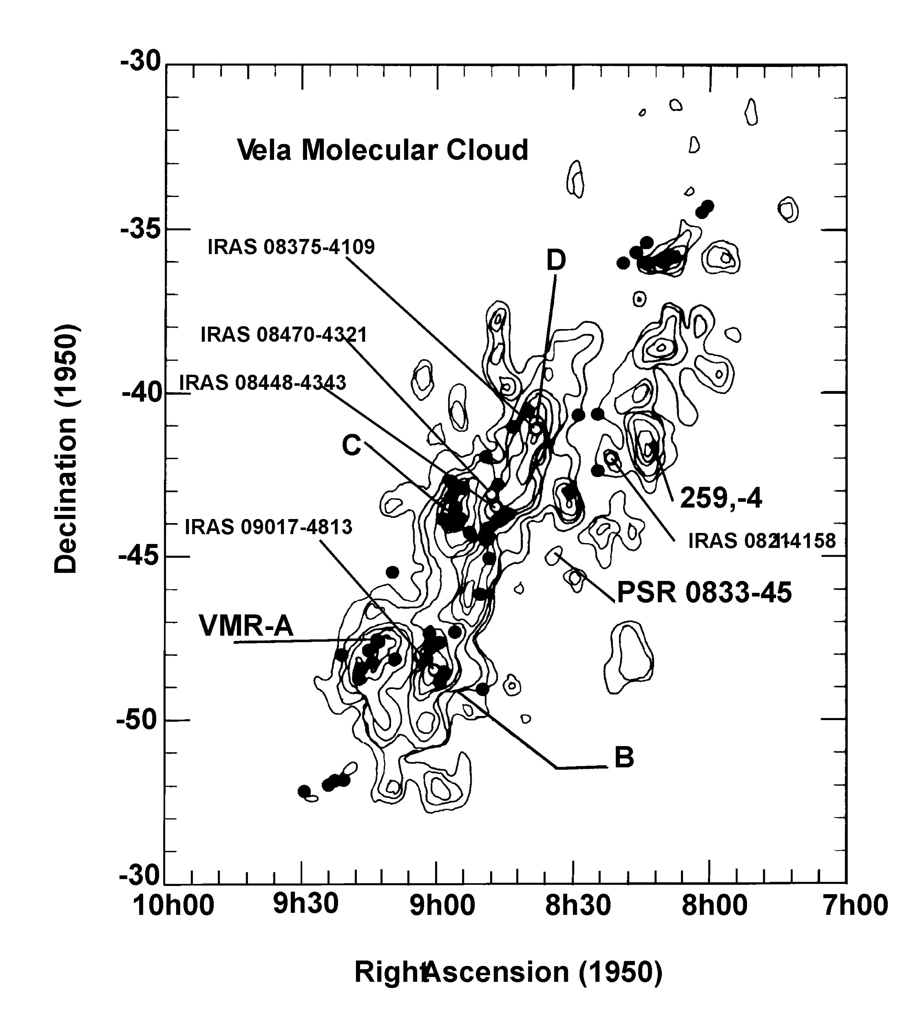
Figure 1: CO (1–0) contour map of the Vela Molecular Cloud complex (Murphy1991A&A...247..202M). The complex is composed of 4 clouds named A, B, C and D in the map. The positions of the observed sources are indicated and the filled circles are the location of the 50 other embedded young stellar objects. Indicated as well are the locations of the Vela Pulsar and the HII region 259,-4. The map is an adaptation of Fig.1 of Liseau1992A&A...265..577L.

2 Protostars in the Vela molecular clouds

We chose to observe 5 intermediate-mass protostars with bolometric luminosities ${L_{*}\sim}$ 100–1000 ${L_{\odot}}$, corresponding to masses of 2–10 $M_{\odot}$ (Palla1993ApJ...418..414P). The characteristics of the objects are summarized in Table 1. These objects are the brightest sources in the $L$- and $M$-band taken from the sample of Class I YSO candidates in the Vela molecular cloud (Liseau1992A&A...265..577L), hereafter LLN. The location of the sources is shown in Fig. 1, together with that of other candidates not studied in this work. Four of these sources have been observed by Pontoppidan2003A&A...408..981P. The Vela molecular cloud is located in the Galactic plane, and is reachable only from observatories in the Southern hemisphere. It lies in an RA range ($\sim$9h) which was not covered by the Infrared Space Observatory (ISO) satellite during the entire mission to avoid damage from the infrared radiation from the Earth.

The complex hosts three supernova remnants (Vela SNR, Puppis A and G266.2 -1.2), the latter discovered by recent X-ray satellites (Aschenbach1998Natur.396..141A). The spectral energy distributions (SEDs) of the objects, red IRAS colors and a near-infrared slope $s\equiv d\log(\lambda F_{\lambda})/d\log(\lambda)\geq 0$ as defined by Adams1987ApJ...312..788A are characteristic of YSOs. Near-infrared imaging has revealed that the chosen targets are the brightest members of their respective proto-stellar clusters (Massi1999A&AS..136..471M). The companion stars observed serendipitously (see Sect. 3) are fainter class I objects. The entire complex was mapped in the CO $J=\!1\!\rightarrow\!0$ transition by Murphy1991A&A...247..202M. The complex is composed of at least four Giant Molecular Clouds (A, B, C and D), with individual masses exceeding 10⁵ $M_{\odot}$, where active star formation occurs. These dark clouds are relatively nearby ($700\pm 200$ pc), therefore giving the possibility to study the ices in a typical galactic environment. The location of the different objects and of their companions coincides with a maximum in the CO $J=\!1\!\rightarrow\!0$ integrated emission and with the highest visual extinction. Extinction studies toward background stars have shown little foreground absorption from diffuse clouds with a maximum of $A_{V}$=3.4 (Reed1990AJ....100..156R). Assuming that the threshold extinction for detection of the water ice feature in this cloud is $\sim$3.3, the amount of water ice that resides in the foreground is negligible. The exact threshold value is unknown for Vela, but it could be much higher than 3.3 (Whittet2003dge..conf.....W).

Table 1: Characteristics of the sources.

		(1)	(2)	(3)	(4)	(5)	(6)	(7)	(8)
Source		$L_{\mathrm{NIR}}$	$L_{\mathrm{MIR}}$	$L_{\mathrm{IRAS}}$	$L_{\mathrm{submm}}$	$L_{bol}$	$M_{\mathrm{env}}$	$A_{\mathrm{V}}$	$N_{*}$
		(%)	(%)	(%)	(%)	($L_{\odot}$)	($M_{\odot}$)	(Mag)	(pc-2)
LLN 8	IRAS 08211–4158	5.3	10.5	53.3	31.0	141  (a)	…	…	…
LLN 13	IRAS 08375–4109	5.3	6.8	72.8	17.7	960  (b)	2.6(b)	$\geq$ 40(a)	800(b)
LLN 17	IRAS 08448–4343	1.3	4.0	60.8	33.9	3100 (b)	6.4(b)	$\sim$ 40(a)	3400(b)
LLN 19	IRAS 08470–4321	4.8	20.3	65.8	9.1	1600 (b)	3.5(b)	$\sim$ 40(a)	2400(b)
LLN 41	IRAS 09017–4716	…	…	80.7	19.3	470	…	…
LLN 20(c)	IRAS 08476–4306	0.5	3.1	66.8	29.7	1600 (b)	2.2(b)		3900(b)
LLN 33(c)	IRAS 08576–4314	2.6	12.6	80.6	4.2	91(a)	…	…	…
LLN 39(c)	IRAS 09014–4736	1.3	5.7	71.1	22.0	807(a)	…	…	…
LLN 47(c)	IRAS 09094–4522	3.4	13.3	74.4	8.9	21(a)	…	…	…

Notes: The dots refer to values which are not available in the literature.

Column 1–4: The fractional luminosities are computed by Liseau1992A&A...265..577L. The indices refer to the wavelength range 1-5 $\mu$m (column 1), 5-12 $\mu$m (column 2), 12-100 $\mu$m (column 3) and 0.1-1 mm (column 4) for NIR, MIR, IRAS and submm, respectively. $L_{\mathrm{submm}}$ are estimated by Liseau1992A&A...265..577L when the millimeter observations do not exist.

Column 5: Bolometric luminosity.

Column 6: The envelope masses ($M_{\mathrm{env}}$) are derived from 1 mm continuum flux by Massi1999A&AS..136..471M for four of our sources. Envelope masses are only given for those sources for which millimeter observations have been carried out.

Column 7: Extinction estimated by Liseau1992A&A...265..577L.

Column 8: $N_{*}$ refers to the maximum stellar surface densities measured.

Reference: ^aLiseau1992A&A...265..577L, ^bMassi1999A&AS..136..471M, ^c VLT-ISAAC data analyzed by Pontoppidan2003A&A...408..981P.

3 Observations and data reduction

The observations were performed using ISAAC mounted on VLT-ANTU in Paranal, Chile, in the $L$ (2.85–4.1 $\mu$m) and $M$ (4.5-4.8 $\mu$m) band in January and November 2001 under mediocre conditions. ISAAC is a cryogenic mid-infrared (1–5 $\mu$m) imaging facility and grating spectrometer. The instrument uses a Santa Barbara 1024 $\times$ 1024 pixel InSb array. The entrance slit of the grating spectrometer was set to 0.6″, which results in a resolving power of 600 in the $L$ band and 800 in the $M$-band (low resolution mode). Since the average seeing at Paranal in the infrared was $\sim$0.6^′′, little flux from the object was lost. The slit was oriented such that the main target and a second nearby object, when present, could be observed simultaneously. An example of an acquisition image at $L$-band is shown in Fig. 2. The companion object is located between 5 and 10″ from the main source. The large detector combined with the 0.6″ slit allowed the entire $L$- and $M$- band to be obtained in one exposure each. The integration times of 30–40 min per object and by band were chosen such that the $S/N$ ratio reaches 60 in the wavelength regions of good atmospheric transmission, allowing an analysis of the profile. Any other absorption features with an optical depth of 0.05 (3$\sigma$) can be detected as well. In complement, three sources LLN 13 (IRAS 08375–4109), LLN 17 (IRAS 08448–4343) and LLN 19 (IRAS 08470–4321) were observed at a resolving power of 10,000 (0.3″ slit) in the $M$-band. A summary of the observations is presented in Table 2.

The objects were observed with a chopping along the slit with a throw of typically 15″ together with nodding. This technique removes the majority of the sky and background noise. After or before each science target, the spectrum of a standard star was obtained with the same setting (BS~3185 of spectral type F6II and BS~3842 of spectral type G8II). The difference in airmass between the target and standard star is always kept less than 0.015. The stars used for atmospheric correction were chosen to be late-type photometric standards. The targets have accurate published photometric measurements (see Table 2) and those values were used to estimate the flux of the main and companion objects. The companions are 3.5 to 18 times fainter than the main sources, which are the brightest objects in their respective proto-clusters. The absolute flux calibration is uncertain by 10%. The standard star spectra were not modeled and therefore hydrogen absorption lines in the spectrum were not removed. In consequence, apparent emission features at 3.04 $\mu$m (HI Pf$\epsilon$ 5-10), 3.30 $\mu$m (HI Pf$\delta$ 5-9), and 3.74 $\mu$m (HI Pf$\gamma$ 5-8) in the data may be spurious features from the rationing by the standard star.

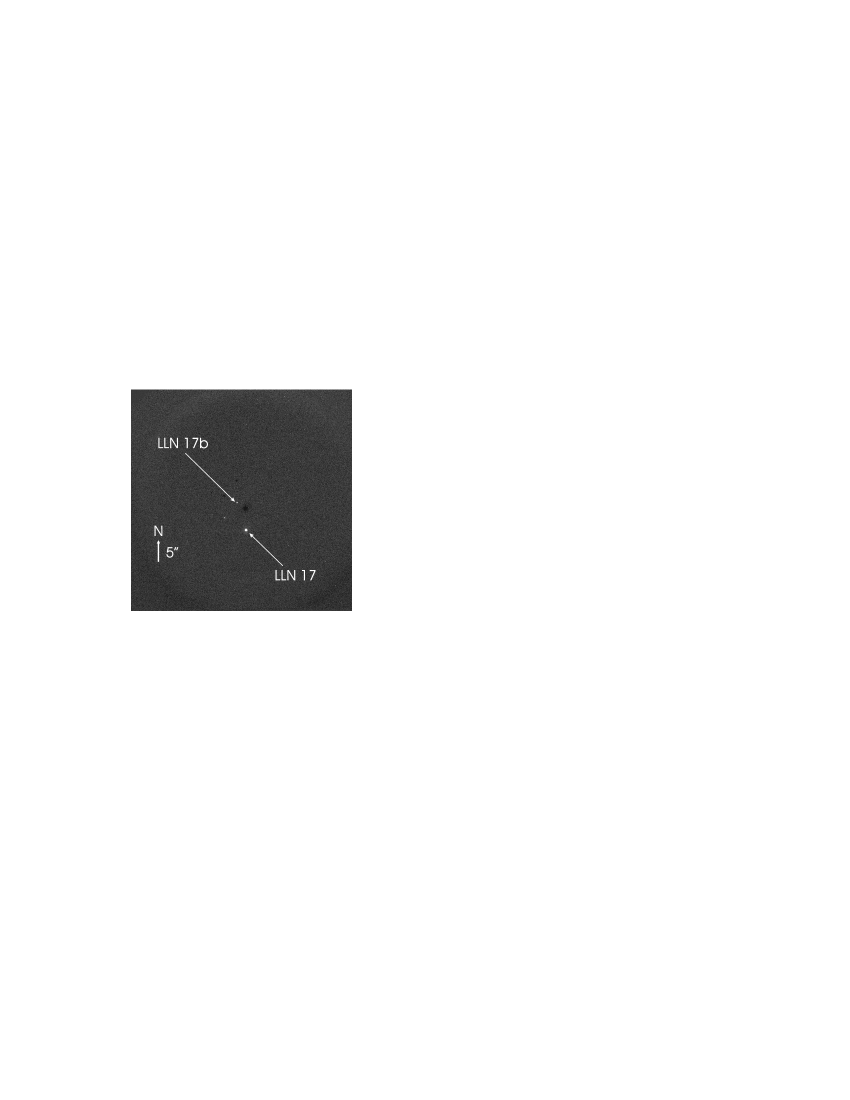
Figure 2: Acquisition image in the stellar field of LLN 17 (IRAS 08448–4343. The orientation of the image (1024 $\times$ 1024 pixels) is North-South and the pixel scale is 1 ″/pixel and corresponds to the length of the arrow. The negative points are the result of the chopping. The main target is called the source IRS 17-57 in Massi1999A&AS..136..471M and the companion object is source IRS 17-40.

The spectra were reduced using in-house software written in the Interactive Data Language (IDL). The data reduction procedure is standard for IR observations (bad pixel maps, flat-fielding, etc.). The distortions of the raw spectra were corrected. In the $L$-band, the wavelength calibration was obtained from arc lamp measurements. In the $M$-band, because of the scarcity of halogen lamp lines in this wavelength range, the spectra were calibrated by comparing the strong atmospheric absorption lines with high signal-to-noise ratio spectra of the atmosphere above Paranal measured by the ESO staff. The data points in the strongest telluric absorption features show the lowest signal-to-noise ratio and were therefore dropped. This is particularly the case for the telluric gaseous methane absorption band around 3.25 $\mu$m. Error bars are omitted in the flux plots for clarity for the $L$-band spectra, but the atmospheric transmission is provided for information in Fig. 3.

Table 2: Summary of the observations and infrared fluxes taken from the literature (The companion objects are located within 30″ from the main source).

	Coordinate		$J$	$H$	$K$	$L^{\prime}$	$M$	Standard	Resolutionb
Source	RA (J1950)	Dec (J1950)	(Mag)a	(Mag)a	(Mag)a	(Mag)	(Mag)a	star
LLN 8	08 21 07.4	$-$41 58 13	13.00	10.12	7.59	4.79	4.01	BS~3185	Low
LLN 8b	08 21 08.1	$-$41 57 44	…	…	…	…	…	BS~3185	Low
LLN 13	08 37 30.8	$-$41 09 29	$>$14.80	12.14	8.95	5.87	5.09	BS~3842	Low, Med.
LLN 13b	…	…	…	…	…	…	…	BS~3842	Low
LLN 17	08 44 48.8	$-$43 43 26	14.0	11.60	9.13	5.77	4.7	BS~3185	Low, Med.
LLN 17b	…	…	…	…	…	…	…	BS~3185	Low
LLN 19	08 47 01.4	$-$43 21 25	14.7	11.92	8.88	4.08	2.73	BS~3185	Low, Med.
LLN 41	09 01 44.0	$-$47 17 19	$>$14.80	11.51	8.15	4.5	3.3	BS~3185	Low
LLN 41b	09 01 42.3	$-$47 16 43	14.1	11.31	9.41	7.3	6.9	BS~3185	Low
LLN 20c	08 47 39.4	$-$43 06 08	$>$14.90	12.73	10.80	7.7	6.2	…	Med.
LLN 33c	08 57 36.8	$-$43 14 35	$>$16.20	14.1	11.16	7.19	5.7	…	Med.
LLN 39c	09 01 26.4	$-$47 36 34	11.79	10.16	8.55	5.64	5.2	…	Med.
LLN 47c	09 09 25.6	$-$45 22 51	11.82	10.10	8.90	5.94	4.8	…	Med.

Notes:
^a Photometry taken from Liseau1992A&A...265..577L.

^b Low resolution $R\simeq$800 in the $L$ and $M$ band; Medium resolution $R\simeq$10,000 in the $M$ band only.

^c Observed by Pontoppidan2003A&A...408..981P.

4 Observational results

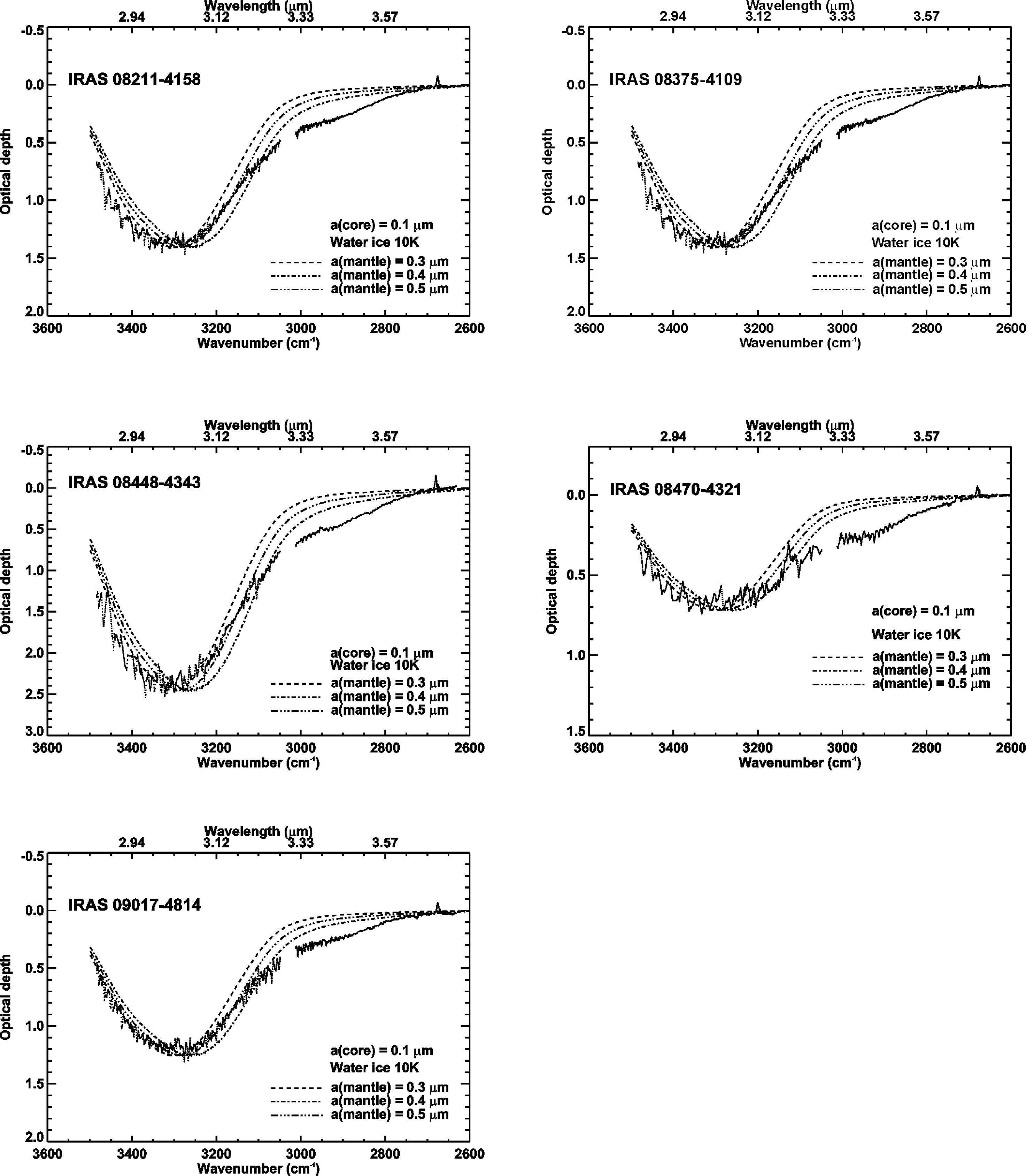
Figure 3: Optical depth profiles of the 3 $\mu$m ice feature for the 5 objects (dotted line) compared to ice coated grains at different radii using laboratory spectra taken from (Hudgins1993ApJS...86..713H).

4.1 Water ice

The spectra of the main objects, converted into optical depth scale, are presented in Fig. 3, while the $L$-band spectra of the companion objects are displayed in Fig. 4 in flux scale. A local blackbody that fits the photometric data at 2.5 $\mu$m and 3.8 $\mu$m, measured by Liseau1992A&A...265..577L was subtracted from the $L$-band spectra to obtain the optical depth scale. The low signal-to-noise ratio in the spectra of the companion objects prevents detailed analysis of the profiles, although column densities can be derived.

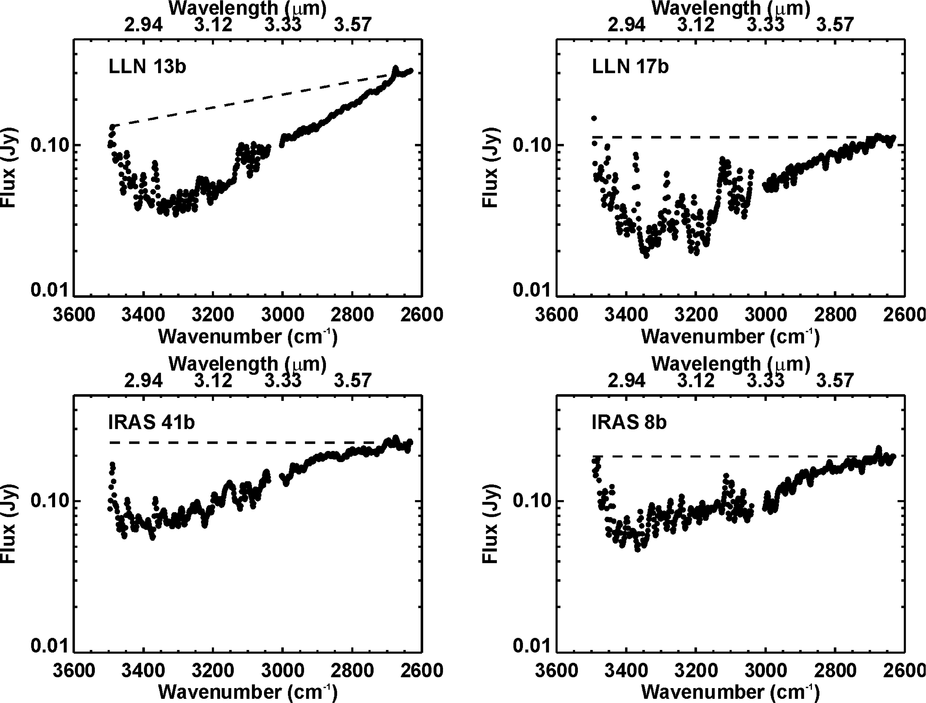
Figure 4: $L$-band spectra of the companion objects. The water ice absorption feature is seen in all spectra. The spectra are dominated by the spurious features due to a bad telluric transmission correction. The dashed lines indicate the adopted continuum used to estimate the water-ice optical depth.

A broad absorption feature extending from 3600 to 2600 cm^-1 (2.85 to 3.8 $\mu$m) is observed in all spectra including the companion objects. This feature, centered around 3.1 ${\mathrm{\mu}}$m, is attributed to the O–H stretching mode of ${\rm H_{2}O}$ ice (e.g., Tielens1983JPhCh..87.4220T). The detection of methanol-ice toward LLN 17 (IRAS 08448–4343) at 3.54 $\mu$m is discussed in Sect. 4.2. The band shape is comparable to that found in quiescent clouds, for example in the line of sight of Elias 16 (Smith1989ApJ...344..413S), a field star located behind the Taurus cloud, which traces unprocessed ices. Table 3 shows the optical depths of the water band for the main and companion objects. The optical depths toward the companion objects are grouped around 1.1 $\pm$ 0.3, whereas a larger scatter is seen for the main objects. In the remainder of this section, we focus our analysis on the main objects.

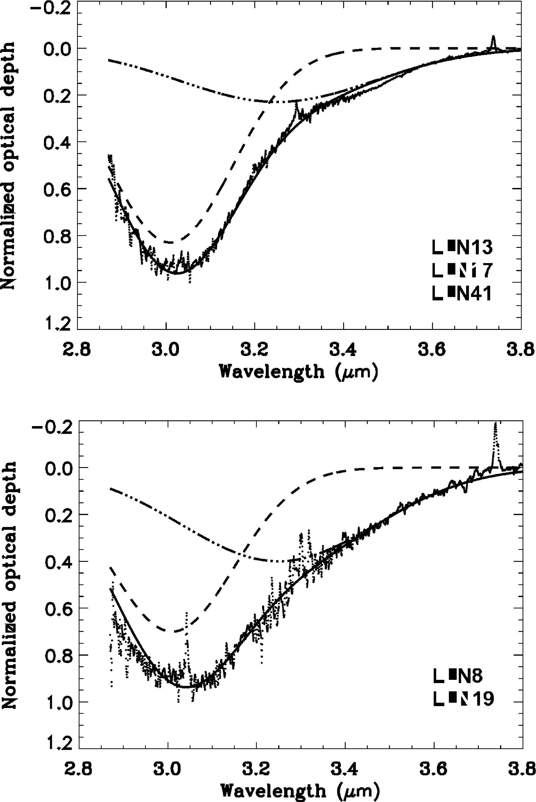
Figure 7: Normalized optical depths of the Vela sources fitted by a combination of 2 Gaussians, one centered at 3.01 $\mu$m, the other one at 3.25 $\mu$m. The upper panel shows the normalized optical depth for 3 Vela sources. The spectra are overplotted one on each other. The similarity between the 3 sources is so strong that it is difficult to separate the sources in the plot. The lower panel shows the spectrum of 2 other Vela sources. The spectra in both panels are fitted by a linear combination of two Gaussians.

An extended wing to the main feature is present in all our sources. The identification of the carrier which gives rise to this long wavelength wing is a long-standing problem (Smith1989ApJ...344..413S; Dartois2001A&A...365..144D). To compare the strength of the wing relative to the main feature, the $L$-band spectra in optical depth scale were normalized to unity at 3.01 $\mu$m. It appears that the spectra can be divided into two groups. The first group is composed of objects where the long-wavelength wing centered at 3.25 $\mu$m is relatively weak compared to the main feature. Three objects fall into this group (LLN 13, LLN 17 and LLN 41). Objects in the second group show a stronger wing relative to the main feature. Two objects in our sample (LLN 8 and LLN 19) pertain to this group. The similarity in the band profile among objects within the same group is remarkable (Fig. 7). In both groups, the entire profile was fitted empirically with a linear combination of two Gaussians centered respectively at 3.01 ($FWHM$=0.14 $\mu$m) and 3.25$\mu$m ($FWHM$=0.44 $\mu$m).

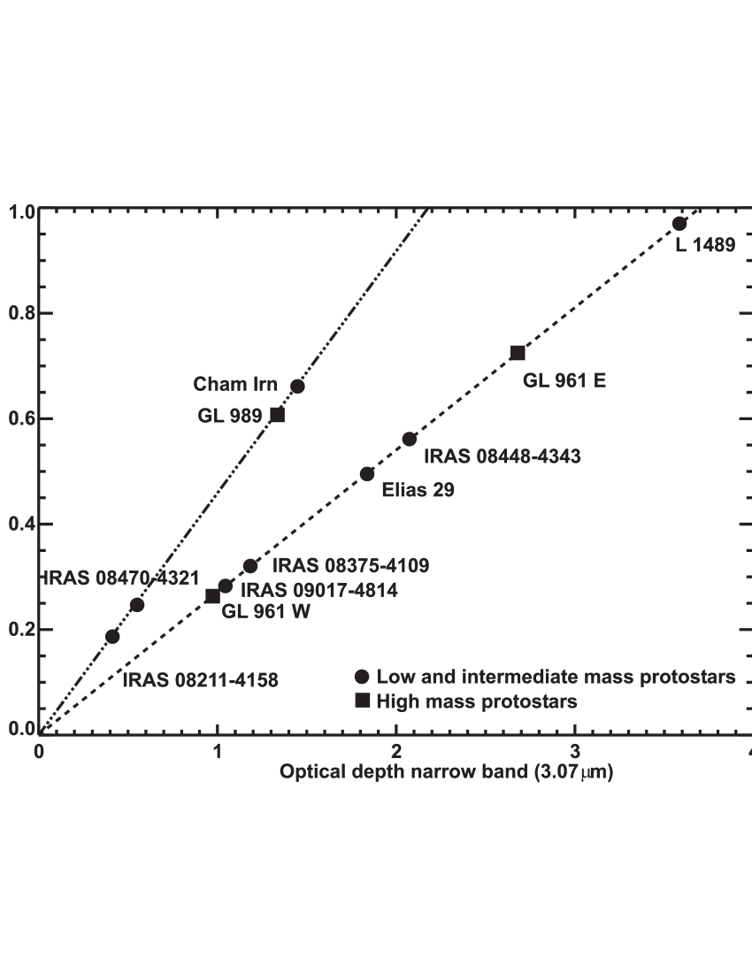
Figure 8: Optical depth at 3.25 $\mu$m versus optical depth at 3.07$\mu$m. The straight lines can be fitted to the data. The origin of both lines is (0,0). The data for sources which are not located in the Vela cloud are taken from the ISO-archive.

A few objects exhibit an additional broad and shallow absorption feature at 3.47 $\mu$m. The optical depth of this feature is reported in Table 3. The 3.47 $\mu$m feature is also found in higher mass protostars (Brooke1996ApJ...459..209B; Brooke1999ApJ...517..883B). The broad 3.47 $\mu$m feature is attributed to an hydrate (e.g. ammonia hydrate, Dartois2002A&A...394.1057D), in which other contributors such as sp³ carbon can be present (Allamandola1992ApJ...399..134A). The optical depth of the main feature at 3.01 $\mu$m is compared to that at 3.25 $\mu$m in Fig. 8. In addition, data of a selected number of other low- and high-mass protostars are included. A strong correlation can be found among objects in each group. The optical depth at 3.25 $\mu$m is found to be 0.27 and 0.45 times that at 3.01 $\mu$m for the two groups, respectively. The tight correlations suggest that the carrier(s) of the extended wing are strongly related to water-ice. However, the correlations may be fortuitous since the number of objects in the sample is limited.

Table 3: Ice column densities. The errors are at 3 $\sigma$ level and are dominated by systematics.

Source		$\tau$(H2Oice)	$N_{\mathrm{ice}}$(H2O)	$T_{\mathrm{ice}}$(H2O)	$N_{\mathrm{ice}}$(OCN-)a	$N_{\mathrm{ice}}$(CH3OH)b
			(1018 cm-2)	(K)	(1016 cm-2)	(1017 cm-2)
LLN 8	IRAS 08211–4158	0.55 $\pm$ 0.10	0.80 $\pm$ 0.15	10–40	$<$1.5	$<$1.0
LLN 8b	IRAS 08211–4158b	1.20 $\pm$ 0.30	1.70 $\pm$ 0.4	10–40	…	…
LLN 13	IRAS 08375–4109	1.40 $\pm$ 0.30	2.20 $\pm$ 0.4	10–40	$<$0.5	$<$1.0
LLN 13b	IRAS 08375–4109b	1.10 $\pm$ 0.30	1.70 $\pm$ 0.4	10–40	…	…
LLN 17	IRAS 08448–4343	2.46 $\pm$ 0.50	3.61 $\pm$ 0.70	10–40	4.3 $\pm$ 0.5	2.5 $\pm$ 1.0
LLN 17b	IRAS 08448–4343b	1.40 $\pm$ 0.3	2.20 $\pm$ 0.2	10–40	$<$1.5	…
LLN 19	IRAS 08470–4321	0.72 $\pm$ 0.100	1.05 $\pm$ 0.2	10–40	$<$0.5	$<$1.0
LLN 41	IRAS 09017-4716	1.26 $\pm$ 0.200	1.85 $\pm$ 0.4	10–40	$<$1.5	$<$1.0
LLN 41b	IRAS 09017-4716b	0.80 $\pm$ 0.30	1.20 $\pm$ 0.4	10–40	$<$1.5	…

Notes:
^a The 3 $\sigma$ upper limits are derived assuming $\Delta\nu$=25 cm^-1 and $A$=1.0 $\times$ 10^-16 cm^-1 molec^-1. Upper limits derived from low resolution spectra are higher than that from medium resolution because of the possible contamination by CO gas phase lines.

^b The 3 $\sigma$ upper limits are derived assuming $\Delta\nu$=14 cm^-1 and $A$=2.8 $\times$ 10^-18 cm^-1 molec^-1. No upper limits are given for the companion objects because the signal-to-noise ratios are too low to provide scientifically meaningful upper limits.

Table 4: Ice abundances relative to water ice.

Source	$N_{\mathrm{ice}}$(H2O)	$N_{\mathrm{ice}}$(OCN-)/	$N_{\mathrm{ice}}$(CH3OH)/	$N_{\mathrm{ice}}$(CO)/
	(1018 cm-2)	$N_{\mathrm{ice}}$(H2O)	$N_{\mathrm{ice}}$(H2O)	$N_{\mathrm{ice}}$(H2O)
		(%)	(%)	(%)
LLN 8	0.80 $\pm$ 0.15	$<$0.2	$<$12.5	$<$22
LLN 8b	1.70 $\pm$ 0.4	…	…	…
LLN 13	2.20 $\pm$ 0.4	$<$0.2	$<$4.5	55
LLN 13b	1.70 $\pm$ 0.4	…	…	…
LLN 17	3.61 $\pm$ 0.70	1.7	6.9	15
LLN 17b	2.20 $\pm$ 0.2	$<$1.1	…	17
LLN 19	1.05 $\pm$ 0.2	$<$0.7	$<$9.5	4
LLN 41	1.85 $\pm$ 0.4	$<$0.1	$<$5.4	22
LLN 41b	1.20 $\pm$ 0.4	$<$1.9	…	$<$15

It has long been realized that light scattering by large ice grains leads to additional extinction on the long wavelength wing of the water band (e.g., Smith1989ApJ...344..413S). Several models of water ice have been developed in which part of the long-wavelength wing is attributed to scattering due to large grains (greater than 0.2 $\mu$m). Our model is similar to that previously used by Smith1989ApJ...344..413S. The silicate core radius is fixed at a constant value of 0.1 $\mu$m. The grain core is coated with a water ice mantle whose thickness is allowed to vary to match the observed spectra. To simplify the problem, the ice is assumed to have a single temperature. The absorption and scattering cross sections are computed using a Mie scattering theory program for coated-spheres (Bohren1983asls.book.....B). The optical constants provided by Hudgins1993ApJS...86..713H for water ice and by Draine2003ARA&A..41..241D for the silicate core were used. The computed spectra for total grain radii of 0.3, 0.4 and 0.5 $\mu$m are shown overlaid on the astronomical spectra in Fig. 3. The peak wavelength of the scattering cross section is red-shifted compared to that of the absorption cross-section and can therefore account for part of the long-wavelength wing. The shape of the long-wavelength wing strongly depends on the actual grain radius. The maximum radius derived from this model is 0.4–0.5 $\mu$m and the ice temperature is below 40 K.

The column densities were estimated by integrating numerically the laboratory spectra over the water band from 2.8 to 3.8 $\mu$m using the band strength for pure H₂O ice of $A$ = 2.0 $\times$ 10^-16 cm molec^-1 at 10 K measured by Hagen1981JChPh..75.4198H:

$$N_{\rm solid}({\rm H_{2}O})=\int\frac{\tau_{\nu}\ d\nu}{A}$$ (1)

where $\tau_{\nu}$ is the optical depth at wavenumber $\nu$ (cm^-1) and $A$ (cm molec^-1) is the integrated absorption cross section per molecule (band strength). The temperature and column densities of the ice giving the best fits are summarized in Table 3. Uncertainties in experimental band strengths for water ice are much lower than that in the determination of the continuum around the water ice band. The inferred column densities varies from 0.8 to 3.6 $\times$ 10¹⁸ cm^-2.

4.2 Methanol ice

Only LLN 17 (IRAS 08448–4343) exhibits a strong methanol feature at 3.54 $\mu$m superimposed on the solid water absorption. The analysis of the methanol feature requires the subtraction of the extended red absorption of the water ice and of the 3.47 $\mu$m. An artificial subtraction of the water ice wing is needed because laboratory mixtures containing methanol ice do not take scattering effects into account. The red-wing continuum is composed of two gaussians whose characteristics are given in Sect. 4.1. The 3.47 $\mu$m feature is modeled empirically by the sum of two gaussians as well ($\lambda_{o}$ = 3.47 $\mu$m, $FWHM$=0.12 $\mu$m and $\lambda_{o}$=3.44 $\mu$m, $FWHM$=0.48 $\mu$m). The remaining feature is compared with mixed ices of H₂O and CH₃OH with different relative abundances. The peak position and the profile of the solid methanol bands are known to vary with the amount of water in the mixture. The presence of water shifts the peak to higher frequency and narrows the methanol band. The best fit is obtained with the mixture H₂O:CH₃OH=10:1. The different components of the fit and the total are shown in the upper limit of Fig. 5. Possible improvement of the fit with a two phase ice is tested. A two phase ice mantle composed of pure methanol and a mixture H₂O:CH₃OH=10:1 in the proportion 30% and 70% respectively improves marginally the fit (Fig. 6).

Adopting the integrated absorption coefficient valid for pure methanol ($A$= 2.8 $\times$ 10¹⁸ cm molec^-1, Kerkhof1999A&A...346..990K), the derived column density of methanol is (2.5 $\pm$ 1.0) $\times$ 10¹⁷ cm^-2 ($3\sigma$), corresponding to a relative abundance compared to water ice of $\simeq$ 6.9 $\pm$ 2%. The search toward the other objects was unsuccessful with an upper limit of $\tau$(CH₃OH)$<$0.02 ($3\sigma$), corresponding to limits on the CH₃OH ice abundances of $\simeq$ 1 $\times$ 10¹⁷ cm^-2 or a limit on the abundance of $<$4.5–12.5%. The methanol ice abundances and upper limits are summarized in Table 4. The relatively high upper limits (4.5–12.5%) stem from the lower water ice abundance in the line of sight of most objects ($N$(H₂O) $<$ 2.3 $\times$ 10¹⁸ cm^-2) compared to that of LLN 17 ($N$(H₂O) = 3.6 $\times$ 10¹⁸ cm^-2).

The detection of solid methanol toward the intermediate-mass protostar LLN 17 (IRAS 08448–4343) with a relative abundance with respect to the water ice of $\simeq$ 6.9% and the non-detection ($<$ 5–10%) toward the other objects can be compared with the variable abundances toward high-mass protostars (from $<$1 % up to $\sim$ 30% in RAFGL 7009S and W33 A; Dartois1999A&A...342L..32D; Brooke1999ApJ...517..883B; Chiar1996ApJ...472..665C; Allamandola1992ApJ...399..134A) as well as low mass protostars ($<$5 up to 25%, Pontoppidan2003A&A...404L..17P). Some of the large variations in the methanol ice abundance occur between objects of similar mass located within the same cluster for low-mass star-forming regions such as Serpens. The upper limits are relatively high because of the low water ice column density found toward most objects. Deeper limits for the LLN sources are needed to determine whether similar CH₃OH ice abundance variations also hold for the Vela star-forming region.

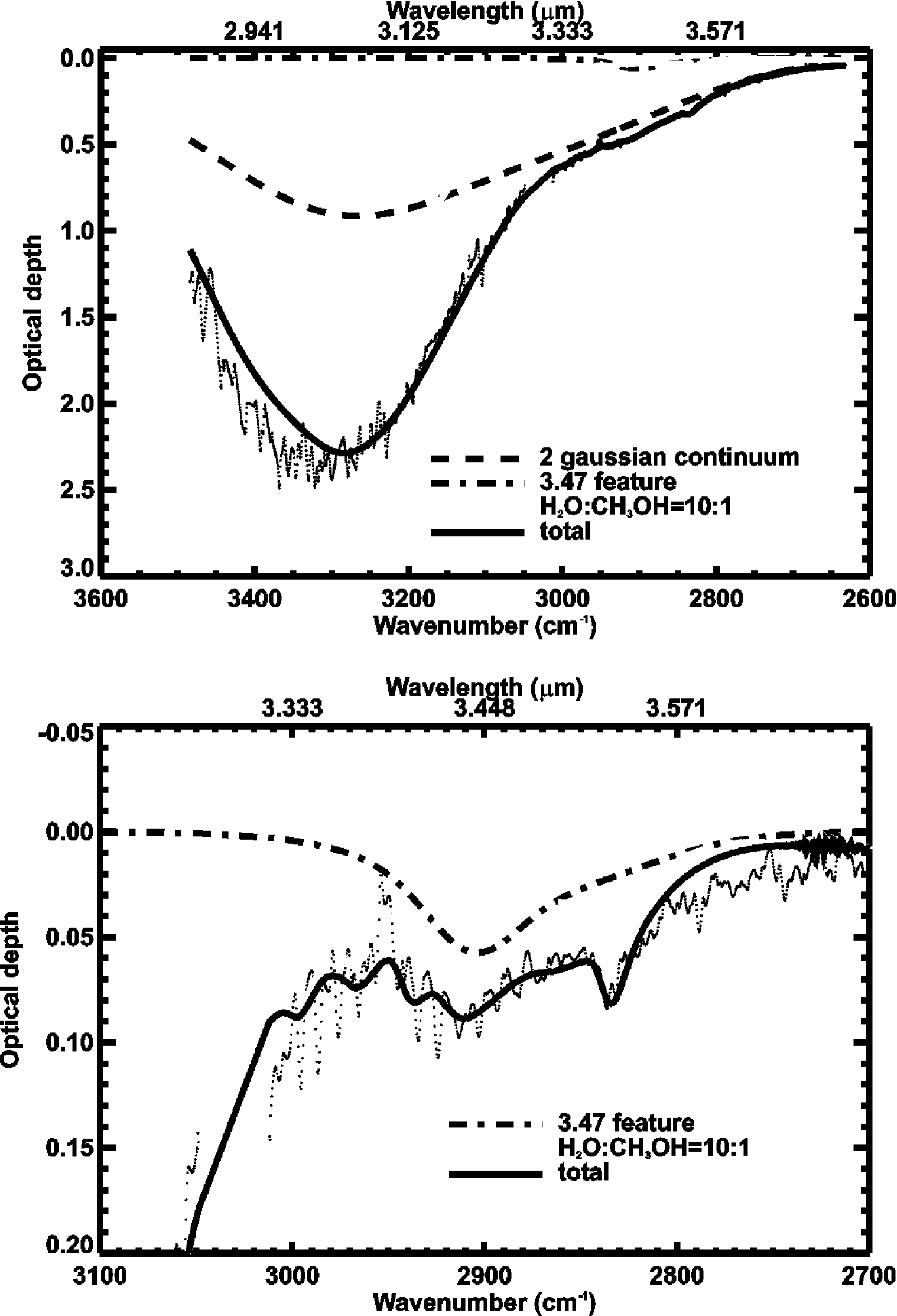
Figure 5: The upper panel displays the water ice feature toward LLN 17. The adopted 2 gaussian continuum, the 3.47 $\mu$m feature and the methanol ice:water ice = 1:10 mixture are overplotted. The lower panel shows a zoom around the methanol feature. In this plot, the 2 gaussian continuum has been subtracted.

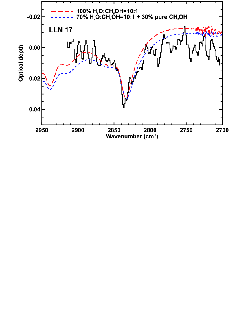
Figure 6: The methanol feature toward LLN 17 is fitted by a single methanol mixture (CH₃OH:H₂O=1:10) and by a 2 component mixture (70% CH₃OH:H₂O=1:10 + 30% pure CH₃OH). The improvement with the 2 component mixture is marginal.

4.3 CO ice

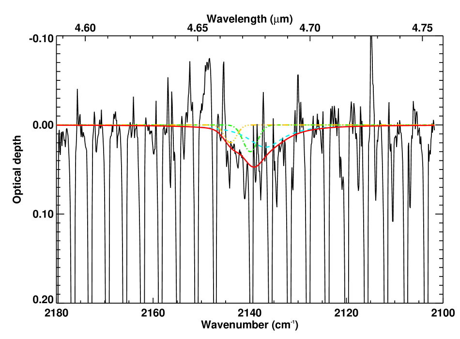
Figure 11: Continuum subtracted VLT ISAAC $M$-band spectrum of LLN~19 around the CO ice feature at 2140 cm^-1 (4.675 $\mu$m). The spectrum is in an optical depth scale. The thick (red) line is the sum of the three fitting components.

In the $M$-band atmospheric window (4.5-4.8 $\mu$m), one can expect to detect the solid CO absorption feature and/or the ro-vibrational band of gaseous CO. A strong feature centered around 4.67 $\mu$m (2141 cm^-1) corresponding to CO-ice is detected in three out of the five sources, namely LLN 13 (IRAS 08375–4109), LLN 17 (IRAS 08448–4343) and LLN 41 (IRAS 09017-4716) and one of the companion objects LLN 17b (IRAS 08448-4343b). Their spectra are plotted in Fig. 9 (open circles). The gas-phase CO ro-vibrational lines can introduce error in the interpretation of the solid feature. In particular, the P(1) line of gas-phase CO lies at the center of the CO-ice band. Medium resolution spectra obtained toward three objects (LLN 13, LLN 17 and LLN19) are presented in Fig. 10. CO ice is detected in the medium , but not in the low resolution spectrum (Fig. 11) toward LLN~19. The cause of the discrepancy is the strong CO gas phase absorption lines, which render the detection of the weak CO ice feature problematic.

In contrast to the water-ice profile, the FWHM of the solid-CO feature differs from source to source (4.6–12.2 cm^-1). The peak positions lie in a narrow range (2139–2141 cm^-1). The FWHM seen toward LLN 13 (IRAS 08375–4109), LLN 41 (IRAS 09017-4716) and LLN 17b (IRAS 08448–4343b) are narrow (4.6–5.8 cm^-1). A narrow width is often observed toward field stars and young embedded low-mass young stellar objects (Pontoppidan2003A&A...408..981P; Chiar1995ApJ...455..234C). The source IRAS 08448–4343 (LLN 17) shows one of the broadest solid CO features ever observed ($\Delta\nu$=12.2 cm^-1). We fitted the spectra using the decomposition outlined in Pontoppidan2003A&A...408..981P who showed that every line-of-sight can be fitted by a linear combination of a narrow middle component (mc), a broad red component (rc) and a blue component (bc). The components are Lorentzian for the red component and Gaussian for the blue and middle components. The central wavenumber and FWHM of each component and their interpretation are given in Pontoppidan2003A&A...408..981P. The phenomenological fits to the spectra allow an astrophysical classification of the sources while more classical fits with laboratory data help in understanding the grain mantle composition as well as the grain shape and size source by source. The best fits are found by a Simplex optimization method (e.g., Press1992nrfa.book.....P). The measurement errors are set constant with wavenumber so that an uniform weight is given to all data points.

The optical depths and derived columns densities are summarized in Table 5, while the abundances relative to H₂O ice are given in Table 4. The solid CO column densities were obtained by integrating numerically the three components. The band strength for pure CO ice was measured to be $A$ = 1.1 $\times$ 10^-17 cm molec^-1 at 14 K (Jiang1975JChPh..62.1201J; Schmitt1989ApJ...340L..33S; Gerakines1995A&A...296..810G). The uncertainties in the measured $A$ value are not taken into account but are smaller than that introduced by the continuum subtraction. Although the band strength shows a 13% variation when CO is mixed with other molecules and a 17% variation with increasing temperature (Schmitt1989ApJ...340L..33S; Gerakines1995A&A...296..810G), the same value for $A$ is adopted to compute the column density for the three components. The errors of $\sim$ 20–30% reflect the noise in the observed spectra and the telluric features removal. Also presented in Table 5 are the CO-ice upper limits for LLN 8 (IRAS 08211-4158). Most of the CO is located in the gas for the latter object (see Fig. 10). The analysis of the gas phase CO lines is presented in a separate paper (Thi et al.  in preparation). The column densities of the middle and red component were estimated by integrating the each band individually. Again, a unique band strength of 1.1 $\times$ 10¹⁷ cm molec^-1 is assumed.

Table 5: CO-ice band optical depth and column density derived from the phenomenological decomposition.

Source	$N_{\mathrm{CO}}^{\mathrm{total}}$	$\tau^{\mathrm{bc}}_{\mathrm{CO}}$	$\tau^{\mathrm{mc}}_{\mathrm{CO}}$	$\tau^{\mathrm{rc}}_{\mathrm{CO}}$	$N_{\mathrm{CO}}^{\mathrm{bc}}$	$N_{\mathrm{CO}}^{\mathrm{mc}}$	$N_{\mathrm{CO}}^{\mathrm{rc}}$	$N_{\mathrm{CO}}^{\mathrm{mc}}$/
	(1017 cm-2)				(1017 cm-2)	(1017 cm-2)	(1017 cm-2)	$N_{\mathrm{CO}}^{\mathrm{rc}}$
LLN 8	$<$11.8	$<$0.10	…	…	…	…	…	…
LLN 13	12.15$\pm$1.71	0.37$\pm$0.12	1.90$\pm$0.12	0.36$\pm$0.12	1.10$\pm$0.39	6.53$\pm$0.15	4.52$\pm$1.62	1.44
LLN 17	5.37$\pm$2.22	0.25$\pm$0.15	0.18$\pm$0.15	0.32$\pm$0.15	0.72$\pm$0.48	0.61$\pm$0.19	4.04$\pm$2.10	0.15
LLN 17b	3.83$\pm$1.74	$<$0.51	1.13$\pm$0.51	$<$0.51	$<$1.5	3.83$\pm$0.58	$<$6.39	$>$0.6
LLN 19b	$<$11.8	$<$0.10	…	…	…	…	…	…
LLN 19c	0.43$\pm$0.05	0.02$\pm$0.005	0.03$\pm$0.005	0.025$\pm$0.005	0.07$\pm$0.02	0.10$\pm$0.02	0.25$\pm$0.05	0.41
LLN 41	4.09$\pm$2.16	$<$0.15	0.48$\pm$0.15	0.18$\pm$0.15	0.14$\pm$0.15	1.64$\pm$0.18	2.27$\pm$2.04	0.72
LLN 41b	$<$11.8	$<$0.10	…	…	…	…	…	…
LLN 20d	5.19$\pm$0.96	0.12$\pm$0.07	0.38$\pm$0.08	0.29$\pm$0.04	0.35$\pm$0.20	1.29$\pm$0.27	3.55$\pm$0.49	0.36
LLN 33d	7.85$\pm$0.81	0.21$\pm$0.05	0.94$\pm$0.09	0.33$\pm$0.03	0.61$\pm$0.14	3.20$\pm$0.31	4.04$\pm$0.37	0.79
LLN 39d	0.44$\pm$0.16	0.004$\pm$0.003	0.02$\pm$0.01	0.03$\pm$0.01	0.011$\pm$0.008	0.068$\pm$0.034	0.37$\pm$0.12	0.18
LLN 47d	$<$10.36	$<$0.06	$<$0.02	$<$0.01	$<$0.17	$<$0.07	$<$0.12	…

^aThe error bars are 3$\sigma$ level.

^bLow resolution spectrum.

^cMedium resolution spectrum.

^dData from Pontoppidan2003A&A...408..981P.

Figure 9: Best fit to the observed spectra using the three components phenomenological decomposition. The observed data points are plotted as open circles. The thick line is the sum of the three components after convolution by the profile of the ISAAC spectrometer ($R\simeq$ 800)..

Figure 10: Medium resolution spectra ($R\simeq$ 10,000) of three objects. The gas phase CO absorption lines are clearly visible and dominate the spectrum of LLN 19.

The line-of-sight toward LLN 13 (IRAS 08375-4109) shows a high middle/red CO ratio typical of CO ice seen toward low-mass protostars and field stars. LLN 41 (IRAS 09017-4716) is also well matched by a high middle/red CO ratio mixture. In contrast, LLN 17 (IRAS 08448-4343) exhibits a stronger red component than a middle one. The CO-ice profile and optical depth is similar to that found toward the high-mass star GL961E (Chiar1998ApJ...498..716C) although the FWHM of $\sim$12.2 cm^-1 is among the largest ever observed. The optical depths and column densities derived from the fits with the phenomenological components are shown in Table 5, together with complementary data obtained from Pontoppidan2003A&A...404L..17P. The total CO ice column densities using fits with laboratory data and phenomenological components are similar within the errors, although the individual components show larger variations.

4.4 The 4.62 $\mu$m ^′′XCN^′′ feature

Other weaker bands can also provide constraints on the energetic processes in the vicinity of young protostars. In particular, the so-called XCN band near 4.62 $\mu$m, contained in the CO survey, has been cited as energetic processes tracer since its discovery toward the massive protostar W33A (Lacy1984ApJ...276..533L). The feature is particularly strong toward LLN 17 (see Fig. 9), and is widely attributed to vibrational stretching modes of -CN groups in molecular coatings on dust grains. The best candidate is the OCN^- ion (e.g., Novozamsky2001A&A...379..588N), as first proposed by Grim1987ApJ...321L..91G. Quantitatively, adopting an integrated band strength $A=$ (4–10) $\times$ 10^-17 cm molecule^-1 for OCN^- (Demyk1998A&A...339..553D), the feature corresponds to a column density of 4.3-11 $\times$ 10¹⁶ cm^-2. Recent laboratory work suggests however that $A$ may be closer to 1.3 $\times$ 10¹⁶ cm molecule^-1 (vanBroekhuizen2004A&A...415..425V). The concentration relative to H₂O using the latter value is $\sim$1%. The derived column density is similar to that found around other YSOs (e.g., Whittet2001ApJ...550..793W; Demyk1998A&A...339..553D). Upper limits are difficult to estimate for the other objects because the wavelength range of the OCN^- feature is dominated by gas phase CO lines in emission or absorption. The upper limits are given in Table 3 and the relative abundances in Table 4. Noteworthy, OCN^- is detected in the object that shows the broadest CO feature, hence the most processed, but has one of the lowest CO/H₂O ratios in our sample. Further discussion on OCN^- in LLN 17 is postponed to Sect. 5.4.

5 Discussion

5.1 Companion objects

Water ice is detected toward four companion objects. The column densities are lower than those toward the primary object, except for LLN8b. The water ice may be located in the outer part of the extended envelope surrounding both the main object and the companion. CO ice has not been detected but the sample is too small and the upper limit too high to allow further discussion, except for LLN~17, which is further discussed in Sect. 5.4.

5.2 Effect of pores on the water ice spectrum

The ice layers on interstellar dust grains may be best simulated by background deposition in the laboratory that forms a porous ice (e.g., Stevenson1999Sci). A porous structure has several advantages over the compact structure as a candidate for interstellar ices. A porous ice can retain a significant amount of molecules such as CO. Moreover, by increasing the temperature, the adsorbed molecules at the surface can migrate into the bulk where they are trapped, i.e., they remain in the mantle even if the grain temperature exceeds the evaporation temperature of the species. The annealing increases the diffusion of molecules into the pores. This point is further discussed in Sect. 5.3.

The effects on the optical constants of a water ice matrix due to isolated (i.e. not connected with each other) inclusions or pores can be simulated using an effective medium theory. One of the formulations is the Maxwell-Garnett approximation (e.g., Bohren1983asls.book.....B for a detailed description). The generalized Maxwell-Garnett formula with ellipsoidal pores is as follows (Niklasson1984JAP....55.3382N):

$$\epsilon_{\rm eff}=\frac{f\epsilon_{\rm ice}(1-\epsilon_{\rm ice})(1-L)+\epsilon_{\rm ice}[L+(1-L)\epsilon_{\rm ice}]}{L+(1-L)\epsilon_{\rm ice}-f(1-\epsilon_{\rm ice})L}$$ (2)

where $\epsilon_{\rm ice}$ is the complex dielectric function of the ice, $f$ is the volume fraction of the inclusion (here the vacuum) and $L$ is the depolarization factor. This factor is equal to $1/3$ for spherical pores and lies between $1/3$ and 1 for prolate spheroidal cavities (long axis along the normal to the layer and to the electric field). By setting $L=1/3$, the classical Maxwell-Garnett formula is recovered. The depolarization factor characterizes the effects of the shape of the pores but does not model the differences in the chemical bonding between a compact and a porous ice. The approximation was used to study the influence of various porosities and the depolarization factor on the simulated spectra. The role of the depolarization factor is studied by keeping all other parameters constant. The resulting spectra are displayed in Fig. 12. The simulations were performed with a porosity of 0.5 (i.e. 50% of the volume is vacuum). It is difficult to estimate the porosity of actual interstellar water ice mantle, but 0.5 is most likely the highest possible value. The generalized Maxwell-Garnett approximation is in theory valid for porosities lower than $\sim$0.3. Simulations with changing the porosity from 0.2 to 0.5 does not result, however, in large differences in the shape of the profile. On the other hand, a small variation in the depolarization factor (e.g. from 0.3 to 0.5) does. In Fig. 12, it can be seen that a higher depolarization moves the peak of the absorption to shorter wavelengths and increases the absorption at higher frequencies compared to that at lower frequencies. This effect may jeopardize the estimate of the ice temperature in Sect. 4.1. The possible ambiguity between a low-temperature and high-temperature ice with different depolarization factors is illustrated in Fig. 12. The simulated shapes are very similar in the blue. The simulations suggest that water ice between 10 and 40 K can fit the observed profiles. However, the 120 K optical constant of porous ice is not able to mimic amorphous cold ice. Porous ice at 120 K lacks absorption in the red but extra extinction can be provided by scattering by large grains. It should be noted that the water ice feature at 3$\mu$m alone does not provide sufficient constraints on the porosity of the ice. Laboratory spectra of water ice at various porosity are warranted to test the validity of the modeling.

It is known that some warm water ice can be hidden in the broad profile (Dartois2001A&A...365..144D). Crystalline H₂O ice was observed in several lines of sight, mostly in the ejected envelope of evolved stars (Smith1988ApJ...334..209S; Maldoni2003MNRAS.345..912M) and in the circumstellar environment of the massive YSO BN object (Smith1989ApJ...344..413S). It is known that the ice mantle on grains around evolved stars is formed by condensation of water molecules synthesized in the gas phase (Dijkstra2003A&A...401..599D), whereas the water ice mantle of interstellar grains is likely created by grain-surface reactions (Nguyen2002MNRAS.329..301N). In conclusion, a significant amount of high-temperature ($T_{\mathrm{ice}}$=40-60 K) ice can be hidden in highly porous ice because of this effect, making the estimate of the water ice temperature from the direct fit to the spectrum unreliable, although there is no direct evidence of highly porous water ice in the ISM. Further theoretical and laboratory investigations are needed to constrain the degree of porosity in ice mantles.

Figure 12: The effects of the depolarization factor $L$ on the water ice feature at 3300 cm^-1 ($\sim$ 3.1 $\mu$m). The effect of porosity for water ice at 120 K is shown ($f$=0 means compact ice while $f$=0.5 means that 50% of the volumn fraction is vacuum. The porous 120 K water ice absorption coefficient is close to the compact 40 K ice.

5.3 Evidence for thermal processing of water and CO ices

The sources chosen for this study were selected among the brightest class I young stellar objects found in the Vela molecular clouds by Liseau1992A&A...265..577L. The objects posses similar characteristics but exhibit a large variations in water and CO ice column densities. It is therefore interesting to find possible relations between the ice properties and the source characteristics. The source characteristics of interest are the extinction $A_{V}$, the infrared luminosity $L_{\mathrm{IR}}$, and colors such as $K-L$, IRAS 12 $\mu$m/25 $\mu$m flux ratio $R$(12/25) and 25 $\mu$m/60 $\mu$m flux ratio $R$(25/60). The ratio $R$(12/25) is a good estimate of the warm dust temperature (100 $<$ $T$ $<$ 250 K), while the ratio $R$(25/60) is sensitive to cooler dust (50 $<$ $T$ $<$ 100 K). Finally, the $K-L$ color allows to probe hot dust ($T>$ 250). The source characteristics were chosen because they are available for all the sources in our sample.

5.3.1 Water ice

The water ice column densities are plotted against the infrared luminosity in the upper left panel of Fig. 13.

Figure 13: Water ice column density $N$(H₂O) versus the infrared luminosity $L_{\mathrm{IR}}$. The error bars are 2$\sigma$ level.

They vary from 0.8 to 3.6 $\times$ 10¹⁸ cm^-2 and do not correlate with increasing infrared luminosity measured between 7 and 135 $\mu$m.

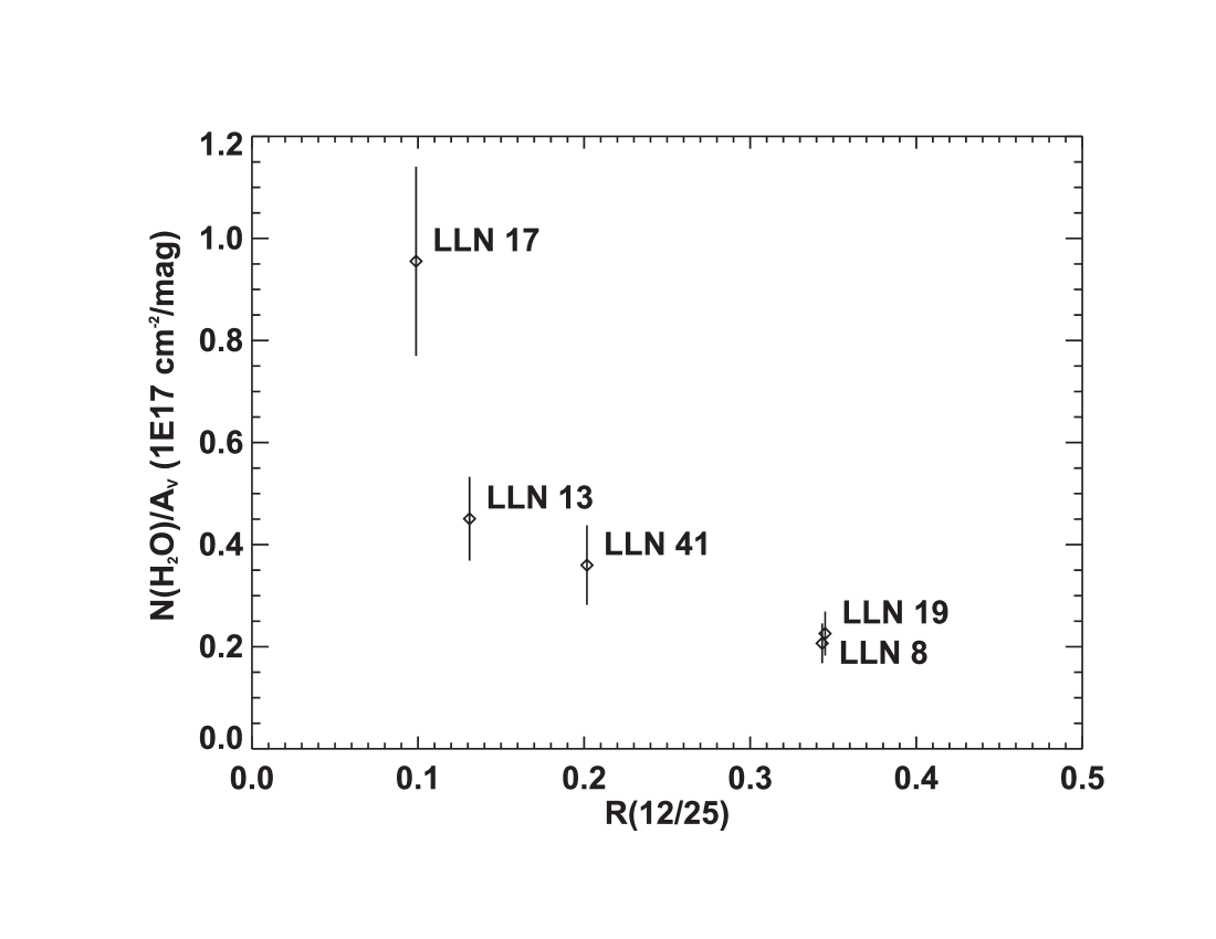
Figure 14: Water ice column density $N$(H₂O) normalized to the extinction A_V versus the ratio $R$(12/25). The error bars are 2$\sigma$ level. The errors on the ratios $R$(12/25) are $\sim$ 5–10 %. A trend is seen between $N$(H₂O)/A_V and $R$(12/25).

The extinction can be estimated from the observed $E(H-K)$ with $A_{\mathrm{V}}$= (15.3 $\pm$ 0.6) $\times$ $E(H-K)$ (Rieke1985ApJ...288..618R). The intrinsic $H-K$ color of early B up to F stars is close to zero. Assuming that the $K$ band flux is dominated by the extincted central source, $E(H-K)$ $\simeq$ $H-K$. The estimated extinction is an upper limit since the $H-K$ color may be lower if emission from hot circumstellar dust at $\sim$ 1500 K dominates the near-infrared continuum. Alternatively, the optical depth at 9.7 $\mu$m (A_V=(18.5 $\pm$ 1.5) $\times$ $\tau_{9.7}$, Roche1985MNRAS.215..425R), measured in the IRAS-LRS spectra, provides a lower limit on the extinction because of potential intrinsic silicate emission. Therefore, the combined use of the two methods brackets the actual extinction. The different estimates of the extinction $A_{\mathrm{V}}$ are provided in Table 6. Liseau1992A&A...265..577L estimated lower limits of 20 magnitudes for most sources in our sample. The discrepancy between the two methods is about a factor 3. In order to better estimate $A_{\mathrm{V}}$, the full Spectral Energy Distribution has been modelled together with the IRAS-LRS data between 9 and 25 $\mu$m of three objects (LLN~13, LLN~17 and LLN~19) using the one-dimensional public radiative transfer code DUSTY (Ivezic1997MNRAS.287..799I) adopting a bare silicate grain model. The three objects were chosen because they have measured 1.3 mm fluxes. The best fits to the SEDs are shown in Fig. 15 and the estimated $A_{\mathrm{V}}$ are given in Table 6. DUSTY fails to fit the details of the silicate feature of (LLN~13, LLN~17), but provides reasonably good fit of the silicate feature for LLN~19. The absorption in 10–25 $\mu$m region of LLN~13 and LLN~17 can be caused by water and CO₂ ice in addition to silicate absorption. The near-infrared and the SED fitting method give relatively close values for $A_{\mathrm{V}}$. Thus, we will adopt the simpler near-infrared method in the rest of the discussion. The $H$- and $K$-band magnitudes are included in Table 1. The derived extinctions using $E(H-K)$ are between 20 and 50, consistent with the values derived from the silicate feature.

Table 6: Estimation of the visual extinction by the 9.7 $\mu$m optical depth, the near-infrared excess and the SED fitting method.

	Method
Source	”$\tau_{9.7}$”	”$E(H-K)$”	”SED fitting”
LLN 8	$>$ 8	$<$ 39	…
LLN 13	$>$ 48	$<$ 59	60
LLN 17	$>$ 13	$<$ 46	40
LLN 19	$>$ 22	$<$ 56	45
LLN 41	$>$ 10	$<$ 40	…

Adopting the relation $N_{\mathrm{H}}$=(1.6 $\times$ 10²¹) $\times$ $A_{\mathrm{V}}$ cm^-2, the derived water ice abundance is (1.3–5.9) $\times$ 10^-5 and is lower than the mean value found in quiescent molecular clouds in Taurus (7 $\times$ 10^-5, Whittet2003dge..conf.....W) and Serpens (9 $\pm$ 1 $\times$ 10^-5, Pontoppidan2004A&ASerpens). The lower water ice abundances found toward the YSO’s in Vela may be ascribed to thermal processing of the dust grains by the central object, lower average gas density, or by external radiation from surrounding YSO’s. Jorgensen2004A&A...416..603J show that variations in the gas-phase abundances in the envelopes of YSOs can be explained by a variable size of the region over which the molecules are frozen out; a similar situation may apply here.

To further ascertain the effect of thermal heating, the water ice abundance $N$(H₂O)/$A_{\mathrm{V}}$ is plotted against the IRAS 12 $\mu$m/25 $\mu$m flux ratio $R$(12/25) in Fig. 14. The IRAS 12 $\mu$m band filter is relatively narrow and therefore, the IRAS fluxes are not strongly affected by the silicate absorption band. The water ice abundance clearly decreases with increasing warm dust temperature. This is consistent with the work of Boogert2000A&A...353..349B, who were the first to show that the color temperature of the dust correlates with ice heating/crystallization through the CO₂ ice bands, which trace CO₂ ice mixed with H₂O ice. The heating of the water ice mantle at $T>$100 K should also results in the formation of a significant amount of heated water ice (narrower profile). However, the water ice observed in our sources is mostly in an amorphous state (see Sect. 4.1), although the narrow feature of warm water ice may be broadened in porous ices (see Sect. 5.2). Alternatively, the inspection of the IRAS-LRS spectra toward LLN~13 and LLN~17 shows that the 12$\mu$m photometry can be biased by water ice absorption. Indeed, the presence of large amounts of water ice with respect to silicate will decrease the ratio $R$(12/25) and explain the trend seen in Fig. 14.

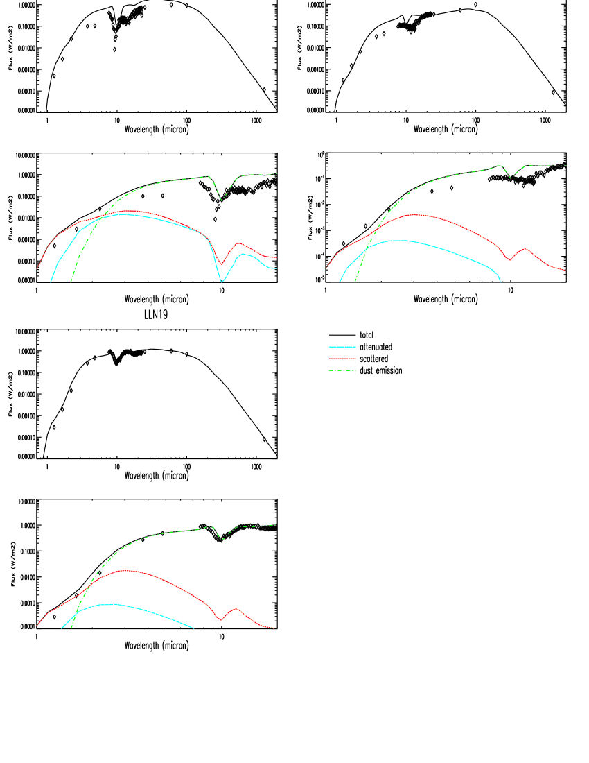
Figure 15: Fit to the SED of LLN 13, LLN 17 and LLN 19. The upper panels show the fit to the entire SED while the upper panels focus on the near to mid-infrared range. Also shown are the contribution by the extincted central object, the dust scattered light and the dust thermal emission.

5.3.2 CO ice

Figure 16: The upper left panel shows the infrared luminosity of the sources computed using the IRAS 4 bands fluxes versus an estimate of the extinction toward the objects. The radius of the circles at the position of each object is proportional to the observed abundance of CO ice. The upper right and lower left panels are two color-color diagrams. The infrared ratios $R$(12/25) and $R$(25/60) are ratios between the fluxes $F$(Jy) at 12 and 25 $\mu$m and between fluxes at 25 and 60 $\mu$m respectively. The lower right panel is a extinction versus $R$(12/25) diagram. The dashed-line represents a possible diving line between presence and absence of CO ice.

In this subsection, we added four objects located in the Vela cloud studied by Pontoppidan2003A&A...408..981P. A closer look at the source characteristics and their possible relationships with CO ice abundance are given in Fig. 16. In this figure, the abundance of CO ice for each object is represented by a circle whose radius is proportional to the CO ice column density. The upper left panel of Fig. 16 shows the line-of-sight extinction $A_{\mathrm{V}}$ and infrared luminosity $L_{\mathrm{IR}}$ of the nine sources.

The total column density of CO ice does not correlate with the infrared nor the bolometric luminosity of the sources. In particular two sources LLN 17 and LLN 19 show similar values for $A_{\mathrm{V}}$ and $L_{\mathrm{IR}}$ but CO ice has only been detected toward LLN 17.

It may be possible to constrain the dust temperature range to which the CO ice abundance is sensitive by finding relations between CO ice abundances and colors. The $K-L$, $R$(12/25), and $R$(25/60) colors encompass dust with temperature ranging from 50 to more than 250 K. This range of dust temperature is well above the CO ice sublimation temperature, thus we do not expect any correlation apart, from perhaps, a weak one with the coolest temperature $R$(25/60). From the two color-color diagrams plotted in Fig. 16 (the upper-right and lower-left panels), it appears that the CO ice abundances vary with the ratio $R$(12/25) but not with $K-L$, which is expected, nor with $R$(25/60), which is more surprising. Before discussing this finding, it is important to test whether the CO ice abundance is related to the extinction in the line-of-sight. Water ice column densities are known to vary linearly with the visual extinction after a certain threshold value (e.g., Whittet2003dge..conf.....W). In other words, water ice abundances do not change with $A_{V}$. For the CO ice in our sample, the abundances do not correlate with $A_{V}$ as testified by the lower-right panel of Fig. 16.

Pure CO ice sublimes at $\sim$20 K, while CO trapped in water ice, often associated with the red component at 2136 cm^-1, evaporates with sudden phase changes of the water matrix at higher temperature (Schmitt1989pmcm.rept...65S; Collings2003ApJ...583.1058C). The amount of CO ice trapped with water should therefore show a similarly decreasing trend as water ice with increasing value of $R$(12/25). The column density of the red component normalized to the estimated extinction $N_{\mathrm{rc}}$(CO)/$A_{\mathrm{V}}$ is plotted in Fig. 17. $N_{\mathrm{rc}}$(CO)/$A_{\mathrm{V}}$ decreases with increasing value of $R$(12/25) . Both $N_{\mathrm{rc}}$(CO)/$A_{\mathrm{V}}$ and $N$(H₂O)/$A_{\mathrm{V}}$ show the same trend with $R$(12/25) and therefore correlate with each other (right panel of Fig. 18). This correlation is consistent with the simultaneous sublimation of water and CO molecules trapped in the water matrix. It is also clear that $N$(CO)/$A_{\mathrm{V}}$ and $N$(H₂O)/$A_{\mathrm{V}}$ do not correlate (left panel of Fig. 18). If $R$(12/25) is another way to express $N$(H₂O)/$A_{\mathrm{V}}$, then Fig. 17 and Fig. 18 express the same relationship between the CO red ice component and water ice.

It is difficult to solely attribute the red component to trapped CO molecules because of the absence in space of the 2152 cm^-1 feature, which is present in laboratory data of CO-H₂O mixtures. However, the 2152 cm^-1 absorption feature seen in laboratory spectra of CO-water mixtures disappears when the dust is heated above $\sim$80 K (Fraser2004MNRAS.353...59F). Other effects may contribute to the red component. One possibility is that part of the red component is due to scattering by the larger grains in the grain size distribution similar to the effect seen for the red wing in the water ice band (see Sect. 4.1 and Dartois2005A&A). In this scenario, the CO and water ice may located in two layers, which ensures that the 2136 cm^-1 feature does not appear even at low temperature. The CO ice trapped in a water matrix and the pure CO ice in large grains may be located in two separate populations in the line-of-sight. The CO red component appears to be a good temperature indicator. The possible relationship between $N_{\mathrm{rc}}$(CO)/$A_{\mathrm{V}}$ and $R$(12/25) should be tested in other star-forming regions. Likewise, future observations of ¹³CO₂ ice will allow to test the possible relation between heated ¹³CO₂ ice and the fraction of hot over cold grains for intermediate-mass YSOs. Spitzer observations of CO₂ ice toward the low-mass protostar HH~46 have shown that most of the ices are located in the cold ($T$ $<$ 50 K) part of a circumstellar envelope, although the inner envelope should be warm enough to explain the presence of a double-peaked absorption feature for the CO₂ bending mode (Boogert2004ApJS..154..359B). The best fit to the CO₂ bending mode feature is obtained with an ice mixture CH₃OH:H₂O:CO₂=0.3:1:1 at 155 K in the laboratory or $\sim$ 75 K in space. This indicates that the inner H₂O, CO₂ and CH₃OH ices are warm.

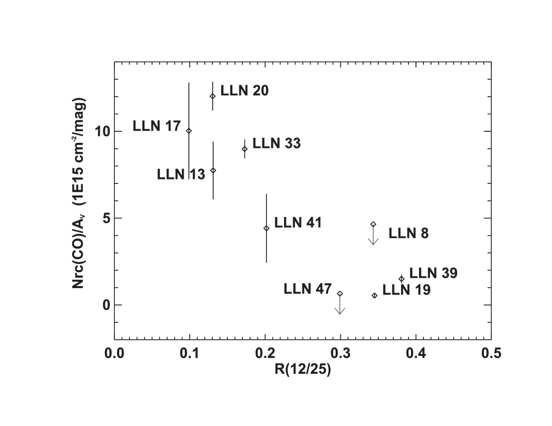
Figure 17: Red component column density $N_{\mathrm{rc}}$ normalized to the extinction A_V versus the ratio $R$(12/25). The error bars are 2$\sigma$ level. The errors on the ratios $R$(12/25) are $\sim$ 5–10 %. A clear trend is seen between $N_{\mathrm{rc}}$/A_V and $R$(12/25).

5.4 Is LLN~17 a peculiar intermediate mass YSO?

Among the intermediate-mass YSOs observed in the Vela Molecular Cloud, LLN~17 is the only object where large quantities of H₂O-rich CO ice, of methanol ice and of OCN^- are found; although it should be emphasized that the relative abundance of methanol ice toward LLN~17 is not extremely high ($\simeq$ 6.9 % w.r.t. H₂O ice). The ice abundances seen toward LLN~17 may be attributed to its peculiar environment. LLN~17 is the most luminous YSO in our sample, it is located in the densest stellar cluster (see Table 1) and shows signs of molecular outflows (Lorenzetti2002ApJ...564..839L; Giannini2005A&A...433..941G). In this section, we discuss whether these particularities can explain the ice abundances.

First we discuss the different ways to form solid-CH₃OH and their implications. The chemistry of solid-CH₃OH is still subject to considerable discussion. The exact moment of its formation and the amount of subsequent energetic processing are currently unknown. Originally it was suggested that methanol ice formed through hydrogenation of accreted CO (Tielens1987ip...symp..397T), but recent laboratory experiments suggest that this mechanism has a very low yield (e.g. Hiraoka2002ApJ...577..265H; Hiraoka2005ApJ...620..542H), although the results are not conclusive (e.g., Watanabe2004ApJ...616..638W; Watanabe2002ApJ...571L.173W). Hydrogen addition to CO at low temperature most likely occurs by H-tunneling since this reaction has an energetic barrier (Woon2002ApJ...569..541W). The original scheme allows an efficient synthesis of methanol ice in cold pre-stellar cores where CO molecule is known to be highly depleted onto grains although the amount of atomic H, which reacts with CO to form CH₃OH, is also small (vanderTak2000A&A...361..327V). If methanol ice is formed at an earlier phase of star formation, probably at the pre-stellar core stage without significant energetic processing afterwards apart from the processing by UV photons generated by cosmic-rays interacting with H₂ and H, similar abundances should be found for members of the same cluster, which is not the case for objects in the Vela molecular cloud and in the Serpens cloud (Pontoppidan2003A&A...404L..17P). Likewise, methanol ice is not present in most lines of sight in the Taurus cloud (Chiar1996ApJ...472..665C). Therefore, methanol ice is probably synthesized at a later stage of stellar collapse where energetic events (UV and/or warm-up in shocks created from the interaction of stellar wind/outflow with the surrounding envelope) from the central object can provide the necessary energy to overcome the reaction barrier. LLN~17 is the most massive YSO in our sample and, hence, the most UV luminous. It would be tempting to attribute the CH₃OH ice to grain surface reactions triggered by UV photons from the central object. However, if we take into account all YSOs where methanol ice has been found, it is also clear that the methanol ice abundance does not correlate solely with the UV flux from the central star and direct stellar UV processing is also not dominant (e.g., Dartois1999A&A...342L..32D; Pontoppidan2003A&A...404L..17P). In addition to the UV from the central star, shocks can produce copious amount of UV photons and heat the gas and dust. Bergin1998ApJ...499..777B have shown that large amounts of water ice can form in post-shock regions. According to this scenario, the water ice mantle is formed by condensation of water molecules formed in the high temperature region of shocks, which subsequently condense rapidly onto the bare silicate grains in the cool post-shock region. In theory, the water ice formed by vapor deposition at T $>$ 100 K should be in the crystalline form. As discussed previously, crystalline water ice is rarely seen toward YSOs. One possibility to circumvent the problem is that high water deposition rate can result in amorphous instead of crystalline ice (Kouchi1994A&A...290.1009K). Another possibility is that crystalline ice is amorphized by cosmic-ray bombardment or Ly $\alpha$ radiation (Leto2003A&A...397....7L). As realized by Bergin1998ApJ...499..777B; Bergin1999ApJ...510L.145B, current gas phase chemical networks do not include all possible high temperature formation paths of methanol. As a consequence, the amount of methanol formed in shocks in standard models is too low to account for the abundance in the solid phase. Another possibility to form efficiently CH₃OH ice is that hot atomic hydrogens created by dissociation of H₂ in shocks impinge onto the grain surface to react with CO to form HCO, H₂CO and finally CH₃OH. Chemical models of shocks that include all formation paths of molecules at high temperature are warranted.

The methanol ice found in LLN~17 is most likely embedded into a water matrix (Sect. 4.2), indicating that water and methanol ice may have formed simultaneously or that methanol molecules have migrated. Interestingly, a collimated bipolar H₂ jet structure composed of bright knots of line emission has been detected toward LLN~17 while neither LLN 19 nor LLN~13 show sign of outflow (Lorenzetti2002ApJ...564..839L). The morphology of the LLN~17 jet points to the presence of episodic phenomena of mass ejection typically observed in protostellar jets (Reipurth1992A&A...257..693R). The molecular outflow has been mapped by Wouterloot1999A&AS..140..177W in the ¹²CO 1-0 transition. Important unknowns in the outflow/shock scenario are the degree of mixing of the processed and unprocessed grains, the precession and the periodicity of the jet phenomenon. In summary, detailed models are needed to determine whether shock chemistry is a viable mechanism to synthesize large amounts of gas and solid phase CH₃OH. Likewise, correlation between outflow and high methanol ice content should be further investigated.

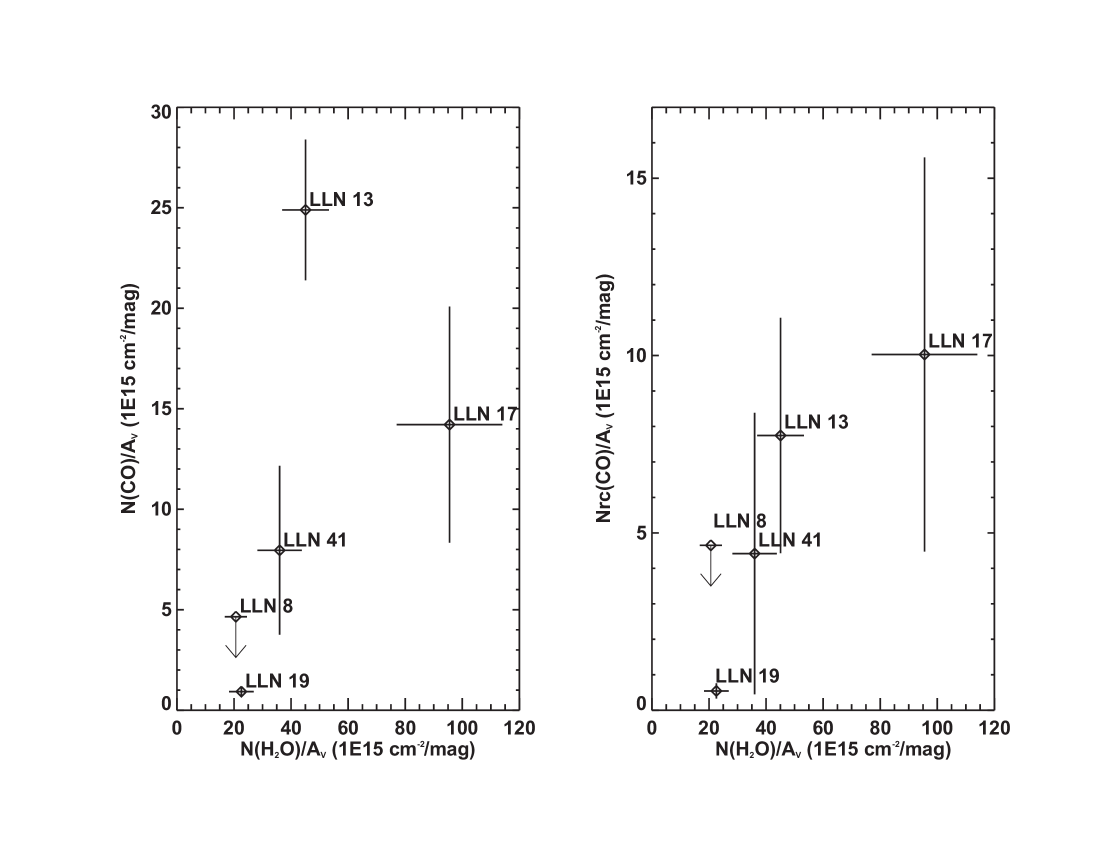
Figure 18: Total CO column density $N$(CO) and red component column density $N_{\mathrm{rc}}$ normalized to the extinction A_V versus $N$(H₂O)/A_V in the left and right panel respectively. A clear trend is seen between $N$(CO)_rc/A_V and $N$(H₂O)/A_V.

It is also interesting to relate the stellar and circumstellar characteristics of LLN 17 to the presence of OCN^- in its envelope. The OCN^- ion is believed to be formed in a solid state acid-base reaction between NH₃ and isocyanic acid (HNCO), efficiently mediated by thermal processing (Demyk1998A&A...339..553D; Novozamsky2001A&A...379..588N; Park2004ApJ...601L..63P; vanBroekhuizen2004A&A...415..425V). The main difficulty in this interpretation is that isocyanic acid ice has never been detected in space, although it has a relatively high gas-phase abundance in hot cores and in shocked regions (Comito2005ApJS..156..127C). The high abundance in shocked regions is consistent with the proposed outflow/shock scenario.

Theoretically, HNCO ice abundance up to $\sim$3% with respect to water ice can also be attained by grain-surface reactions (Hasegawa1993MNRAS.263..589H). Alternatively, an abundance of $\sim$1% for OCN^- can be easily reached by UV-photolysis of the initial mixture H₂O/CH₃OH/NH₃=100:15:15 (vanBroekhuizen2004A&A...415..425V). Although the required amount of UV-dose (fluence) exceeds the value estimated in dense clouds, the large amount of processed CO and CH₃OH ice found toward LLN~17 suggests that the UV field around LLN~17 may be enhanced compared to that provided by cosmic rays induced only. The abundance of NH₃ in the envelope around LLN~17 is difficult to estimate owing to the poor signal-to-noise ratio of the spectrum around the ammonia feature at 2.97 $\mu$m. However, sufficient amounts of NH₃ may have existed in the ice mantle since the 3.47 $\mu$m feature is relatively strong toward LLN~17, assuming that the 3.47 $\mu$m feature is caused by ammonia hydrate. Noteworthy, the detection of OCN^- is often concomittent with that of CH₃OH ice (see Table 5 of vanBroekhuizen2004A&A...415..425V and the references therein).

Another particularity of LLN~17 is that the water ice abundance with respect to H₂ is the highest (see Fig. 18) in our sample. Methanol ice and OCN^- are often detected in objects with high water ice abundance (vanBroekhuizen2004A&A...415..425V; Pontoppidan2003A&A...404L..17P; Dartois1999A&A...342L..32D).

Finally, the presence of water-rich CO ice in LLN~17 and its absence in the companion object LLN~17b as seen in Figure 9 reinforces the idea that the processing occurs in the vicinity of the central object (i.e. with a few thousand AU). The $M$-band spectrum of LLN~17b is too low to give meaningful upper limit on the amount of OCN^-. The difference between LLN 17 and its companion suggests that external heating and/or UV processing by the other stars in the cluster play a minor role (see last column of Table 5).

Interestingly, the OCN^- and methanol abundances relative to water in LLN~17 are close to those found in the envelope around HH 46 (Boogert2004ApJS..154..359B). Likewise, the water-rich CO abundance dominates over the water-poor CO and water ice is relatively abundant (5.7 $\times$ 10^-5).

In summary, the simultaneous presence of large amount of water-rich CO ice, CH₃OH ice , and OCN^- ice toward LLN~17 and the non-detection in other objects are consistent with the idea that these species are formed by a combination of UV and thermal processing in the inner regions of the circumstellar envelope. The UV radiation can be generated by the interaction between the outflows and envelope, by the central source, or by a combination of both mechanisms. Another possibility is that CH₃OH is first synthesized in the gas-phase, then condenses onto grains simultaneously with H₂O in post-shocked regions.

6 Conclusions

We have obtained $L$- and $M$- band spectra of a sample of intermediate-mass protostars in the Vela molecular cloud with the VLT-ISAAC. This is the first significant sample of intermediate mass protostars for which ice data are published.

A broad absorption feature at $\sim$3.01 $\mu$m is detected in all sources (main and companion objects). The features show an extended wing beyond 3.25 $\mu$m, which can be reproduced in part by scattering by grains at radius 0.4–0.5 $\mu$m. The water ice feature is dominated by absorption from cold amorphous ice although the spectroscopic signature of warm water ice can be masked if the ice is porous.

Methanol ice is only detected around the protostar LLN 17 (IRAS 08448–4343). The derived abundance is 10 $\pm$ 2 % relative to water ice. The upper limit on the methanol abundance toward the other sources is between 5 and 10% with respect to water ice.

Solid CO is detected in four main objects and one companion object. The profiles show a large variety of shapes. A strong variation of the total CO ice column density is found. We decompose the CO ice feature into three components. The column of CO becomes significant (i.e. larger than 10¹⁷ cm^-2) only at $R$(12/25) greater than $\sim$0.3. The color $R$(12/25) may trace the abundance of water ice with respect to silicate. There is no clear trend between the column density of pure CO ice, traced by the middle component, and other characteristics of the YSOs ($L_{\mathrm{bol}}$, A_V, IRAS bands flux ratios). On the other hand, we find a possible correlation between the ratio of the flux at 12 $\mu$m and 25 $\mu$m, $R$(12/25), which is a measure of the warm dust temperature (100$<$ $T$ $<$ 250 K), and the amount of CO ice trapped in a water rich ice mantle, traced by the red component. Likewise, the amount of CO ice trapped in a water and that of water may correlate. This possible correlation is consistent with the idea that the water ice and the CO embedded in it sublime simultaneously.

These possible correlations should be tested in other star-forming regions. However, CO ice trapped in water-rich ice cannot solely account for the large amount of CO in the red component seen toward YSOs in Vela. Other factors such as scattering by the larger grains in the size distribution can probably contribute to the red component.

A strong absorption feature centered at 4.62 $\mu$m is detected toward LLN 17 (IRAS 08448–4343). The feature is likely caused by OCN^-. The derived abundance relative to water is 1 $\pm$ 0.2 %. This feature is not detected in any other object in our sample. Together with the detection of methanol and the broad CO feature, the detection of OCN^- suggests that the ice has been thermally and/or UV processed in LLN 17. The processing generated by UV from the central object is not essential and perhaps shocks induced processing is at play. Further theoretical investigations on the possibility to form large amounts of methanol ice together with water ice in post-shocked regions are needed.

Observations of a larger sample of high signal-to-noise ratio spectra obtained with 8-10 meter class telescopes (VLT, Gemini, Keck) and with Spitzer at longer wavelengths of protostars of varying luminosities combined with sophisticated laboratory experiments will improve our understanding of the nature of the ices and their role in the synthesis of complex molecules in the interstellar medium.