Cosmic microwave background multipole alignments in slab topologies

Abstract

Several analyses of the microwave sky maps from the Wilkinson Microwave Anisotropy Probe (WMAP) have drawn attention to alignments amongst the low-order multipoles. Amongst the various possible explanations, an effect of cosmic topology has been invoked by several authors. We focus on an alignment of the first four multipoles ($\ell=2$ to $5$) found by Land and Magueijo (2005), and investigate the distribution of their alignment statistic for a set of simulated cosmic microwave background maps for cosmologies with slab-like topology. We find that this topology does offer a modest increase in the probability of the observed value, but that even for the smallest topology considered the probability of the observed value remains below one percent.

I Introduction

Several recent analyses of the WMAP satellite maps have pointed out an unexpected degree of alignment between the low-order multipoles of the cosmic microwave background (CMB) anisotropy TDH ; DTZH ; Eriksen2003 ; Eriksen2004a ; Hansen ; Biel ; LM ; CHSS ; BMRT . Various explanations have been put forward for these alignments, ranging from statistical fluke or foreground contamination through to a genuinely cosmological interpretation in terms of breakdown of statistical isotropy. Such a breakdown would be a natural consequence of the Universe possessing a non-trivial topology of characteristic scale comparable to the observable Universe (for a selection of cosmic topology review papers see Ref. reviews ).

In this paper, we do not seek to address the interpretation of the observational data, but rather aim to test whether or not slab-space cosmic topologies give rise to the kind of alignments that are tentatively reported to have been observed in the first-year WMAP data. The observational indication is that there exists a preferred direction for the low multipoles. For instance, Tegmark et al. TDH and de Oliveira-Costa et al. DTZH noted that the quadrupole and octupole were closely aligned with one another, and approximately planar. Land and Magueijo LM (hereafter LM) sought the alignment for each multipole $\ell$ that maximized the proportion of power contributed by a single $m$ mode, and noted that the alignments of the first four multipoles were much closer than would be expected under statistical isotropy. These authors have all suggested that such alignments may be an indication of a slab topology where only one dimension is compact (finite and unbounded).

The principal aim of this paper is to determine whether the LM alignment is a prediction of slab-space cosmic topology. We simulate CMB maps for spatially-flat slab topologies, for different sizes of the compact dimension, and derive the statistics of the alignments as defined by LM. We find that the degree of alignment in the observed data remain anomalous even in slab-space topologies.

II Cosmic Topology and the CMB

If the Universe has a non-trivial topology, that would lead to a breakdown of global isotropy. The spherical harmonic expansion coefficients $a_{\ell m}$ of the observed map of CMB temperature anisotropies would then no longer be uncorrelated random variables, their correlation matrix having off-diagonal terms. Riazuelo et al. Riazuelo04a ; Riazuelo04b found this correlation matrix for many multiconnected spaces, by computing the eigenmodes of the Laplacian with boundary conditions reflecting the particular topology.

Let us briefly recall how this is done. The power spectrum coefficients, the $C_{\ell}$, are computed via the formula

$$C_{\ell}\propto\int\Theta_{\ell}^{2}(k)P(k)k^{2}\;{\rm d}k\,,$$ (1)

where $P(k)$ corresponds to the initial power spectrum of cosmological perturbations of wavenumber $k$, and $\Theta_{\ell}(k)$ are transfer functions defined in Ref. huwhite95 .

In the case of Gaussian perturbations, the full statistical information is encoded within the two-point correlation function. The observable quantities correspond to the $a_{\ell m}$ coefficients of the decomposition of the temperature field in spherical harmonics. The quantity we are interested in is therefore the correlation matrix $\left<a_{\ell m}a^{*}_{\ell^{\prime}m^{\prime}}\right>$. In a simply-connected Universe, the cosmological principle implies that the cosmological perturbations must be statistically isotropic. This in turn implies that the above correlation matrix is necessarily diagonal: $\left<a_{\ell m}a^{*}_{\ell^{\prime}m^{\prime}}\right>=\delta_{\ell\ell^{\prime}}\delta_{mm^{\prime}}C_{\ell}$, where $C_{\ell}$ is defined above. In the case of a multi-connected Universe, the Universe is no longer isotropic and the correlation matrix has non-zero off-diagonal components.

In a spatially-flat multi-connected Universe, the eigenmodes of the Laplacian $\Upsilon^{k}_{s}$ can be decomposed into the usual basis of spherical harmonics and spherical Bessel functions as

$$\Upsilon^{k}_{s}=\xi^{k}_{s\ell m}\,j_{\ell}(kr)Y^{m}_{\ell}(\theta,\varphi)\,,$$ (2)

where the index $s$ distinguishes between modes with identical wavenumber $k$. With this decomposition, the coefficients of the correlation matrix read

$$\left<a_{\ell m}a^{*}_{\ell^{\prime}m^{\prime}}\right>\propto\sum_{k,s}\xi^{k}_{s\ell m}\xi^{k}_{s\ell^{\prime}m^{\prime}}{}^{*}\Theta_{\ell}(k)\Theta_{\ell^{\prime}}(k)P(k)\,.$$ (3)

Once the $\xi^{k}_{s\ell m}$ coefficients are known, all the statistical information about a given topology can be computed using an existing CMB code. This method therefore naturally takes into account all the contributions (Sachs–Wolfe, Doppler and Integrated Sachs–Wolfe (ISW)) to the temperature anisotropies, unlike the analytical formula of Ref. DTZH which performs an estimate of the Sachs–Wolfe term only in the large-wavelength limit.

Should one take into account the Sachs–Wolfe contribution only, then the CMB maps would exhibit sets of pairs of circles whose temperature pattern would perfectly match. These correlated temperature patterns arise from the fact that we see two copies of the same region along different lines of sight. The Doppler and ISW contributions reduce this correlation because the Doppler term depends on the direction in which the electron velocity field is observed, and the ISW effect depends on the photon history along the line of sight CDS . The simulated maps neglect reionization. As with the ISW effect, reionization tends to blur the topological signature in the correlation matrix, so that our simulated maps exhibit a stronger departure from statistical isotropy than more realistic maps.

Following LM’s suggestion, we restrict our study to slab spaces. Our computational method requires all directions to be finite, so we chose rectangular tori with dimensions of the form $15\times 15\times X$, labelled T$[15,15,X]$ in the notation of Kunz et al. Kunz2005a , where $X=1,2,...,15$ and the sizes are in Hubble radius units. Recall that the distance to the last-scattering region today is around $3.1$ Hubble radii in a flat $\Lambda$CDM model with $\Omega_{\Lambda}\simeq 0.7$. The dimensions of size 15 Hubble units are essentially infinite, which we checked by comparing the correlation matrix of T$[15,15,15]$ to that of a standard simply connected, infinite universe. Hence T$[15,15,X]$ is a computationally-favourable approximation to a slab space (that is, a space with only one compact dimension). Another reason to consider slab spaces is that matched circles searches have so far given negative results starkman , so that it seems likely that only topologies exhibiting a small number of circles, such as slab spaces, are compatible with the data.

III Results

III.1 The Land–Magueijo statistic and its observed value

LM devised a statistic to study the alignments of multipoles. For each multipole, they found the orientation of the coordinate axes which maximized the concentration of the multipole power into a single $m$, defining

$$r_{\ell}=\max_{m,{\bf n}}\frac{C_{\ell m}}{(2\ell+1)C_{\ell}}\,,$$ (4)

where ${\bf n}$ is the coordinate axis orientation, $C_{\ell}$ the usual power spectrum, and $C_{\ell m}$ measures the power at a single $m$ value, defined as $C_{\ell 0}=\left|a_{\ell 0}\right|^{2}$ and $C_{\ell m}=2\left|a_{\ell m}\right|^{2}$ for $m>0$. The vector ${\bf n}_{\ell}$ is defined as the one which provides the maximum value of the statistic $r_{\ell}$ for each $\ell$.

They noticed a strong alignment of the ${\bf n}_{\ell}$ of the lowest four multipoles, $\ell=2$,…,$5$ and quantified this by defining the mean angle between the six different pairs of alignments. As the orientation vectors are headless (the same results are achieved by interchanging ${\bf n}_{\ell}$ with $-{\bf n}_{\ell}$), one must choose the angle $\theta_{ij}$ which is less than 90 degrees. The average alignment angle is then

$$\hat{\theta}=\mathrm{mean}\left(\theta_{ij}\right),\quad i,j=2,3,4,5\;\mbox{with}\;i\neq j\,.$$ (5)

They evaluated this alignment angle for the Tegmark, de Oliveira-Costa, Hamilton (TOH) cleaned and Wiener filtered maps of Ref. TDH and found the values of $22.4^{\circ}$ and $22.3^{\circ}$ respectively. We have confirmed this result using the code described below.

For a Gaussian map, the predicted value of $\hat{\theta}$ is one radian. This arises as follows. Remembering that the alignment direction is a headless vector, the average separation between two such vectors can be found by rotating coordinates so that one is at the north pole. The other then has one end uniformly distributed in the northern hemisphere, so the average angle is given by the average distance of a point in the northern hemisphere from the north pole, which is one radian.

Land and Magueijo found that the low observed value arose in only 5 out of 5000 simulated Gaussian maps, a result which we confirm below. On the face of it, this strongly excludes statistical isotropy, but one does need to bear in mind the strong a posteriori selection of their statistic; for instance the signal would be much weaker if the average angle included alignment with even just the sixth multipole.

It is also found that because the statistic involves maximization, it can be highly sensitive to small changes in the map, because multipole concentrations can have near double maxima for different $m$, giving completely different alignment directions. For example, while in the result above using the TOH maps, the quadrupole alignment was one which maximized the $m=2$ multipole, with ${\bf n}_{2}$ in the direction $(b,l)\approx(60,-100)$, we find (as did LM) that for the Lagrange internal linear combination map (LILC) produced by Eriksen et al. Eriksen2004a a completely different orientation is selected for the quadrupole, this time maximizing the $m=0$ multipole (in the TOH map this maximum is just slightly less than the one chosen), which significantly increases $\hat{\theta}$ to $55.2^{\circ}$. Similarly, in the case of the internal linear combination map (ILC) produced by the WMAP team Bennett03 , while the preferred axis of the quadrupole is similar to that in the TOH maps, this time it is the direction of the octupole that is the cause of a discrepancy that increases $\hat{\theta}$. We note this as a caveat; in both these cases of near double maxima, three of four maps agree as regards the direction of the preferred axis for the concerned multipole. The maps differ in the details of how foregrounds are removed from them.

Again, we do not here seek to address data-related aspects such as the likelihood of finding the observed $\hat{\theta}$ given the uncertainties in foreground subtraction, the sky-cut, cosmic variance etc. While these issues are important to consider when determining whether the claimed detection of a breakdown of isotropy is significant, papers that reported the detections in the first place have delved into such questions to some extent, and there is only limited progress one can make with an a posteriori detection. Aspects of foreground contamination have been studied in Refs. CHSS ; Eriksen2004a ; Biel2 ; Vale ; MC . For instance, Copi et al. CHSS considered the nature of known foregrounds without finding any clear connection to low-$\ell$ alignments, at least as regards the LM kind.

Despite the above-mentioned caveats, the value of $\hat{\theta}$ found by LM is very low, and they speculate that it may be a signature of slab topology, already invoked in Refs. TDH ; DTZH as a possible explanation of the quadrupole and octupole planarity. Our aim is to test this suggestion by evaluating the distribution of the $\hat{\theta}$ statistic for simulated slab topology maps, and checking whether, relative to the case of a trivial topology, such topologies can better explain a low $\hat{\theta}$.

III.2 The Land–Magueijo statistic for simulated maps of slab topology

Given the full ensemble average correlation matrix $\langle a_{\ell m}a^{*}_{\ell^{\prime}m^{\prime}}\rangle$ of the spherical harmonic coefficients for slab space topologies of form T$[15,15,X]$, we create corresponding random realizations of the $a_{\ell m}$. These are then rotated through a two-dimensional grid of galactic angles $b$ and $l$ (we used spacings of one degree in each). The $a_{\ell m}$ transform under rotations as (see e.g. Ref. CDEW )

$$a_{\ell m}=\sum_{m^{\prime}=\,-\ell}^{\ell}a_{\ell m^{\prime}}e^{-im\alpha}d_{m\,m^{\prime}}^{\,\ell}(\beta)e^{-im^{\prime}\gamma}\,,$$ (6)

where ($\alpha,\beta,\gamma$) are the Euler angles corresponding to the rotation, and $d_{mm^{\prime}}^{\ell}(\alpha,\beta,\gamma)$ is part of the representation of the Wigner rotation matrix CDEW . Rotating the $a_{\ell m}$ over the entire grid, the rotation $\mathbf{n}_{\ell}$ (and associated $m$) that maximized $r_{\ell}$ was recorded, for each $\ell$. Thus $\hat{\theta}$ was found for each simulation. This was repeated for an ensemble of universes so that the distribution of $\hat{\theta}$ was built up. The ensemble average value $\langle{\hat{\theta}}\rangle$ was also found. This was then repeated for different dimensions $X$ of the rectangular toroid T$[15,15,X]$.

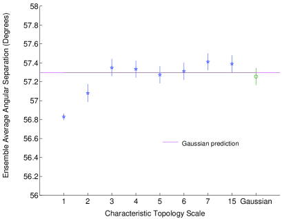
Figure 1: The ensemble average alignment $\langle{\hat{\theta}}\rangle$ and its standard error for the T$[15,15,X]$ topologies, as a function of topology scale $X$. The horizontal line is the Gaussian prediction.

Figure 1 shows the ensemble average values $\langle{\hat{\theta}}\rangle$, together with their standard error, against $X$. For Gaussian maps, the expected result of one radian is accurately recovered. We further see that the large-scale topology maps behave essentially as Gaussian maps. Only for $X<3$ do we begin to see an effect of topology, with the ensemble average reducing slightly with respect to the Gaussian result. The shift is very small as compared to the observed value of $\hat{\theta}$.

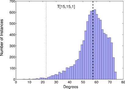
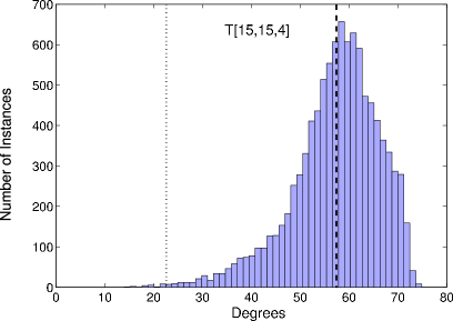
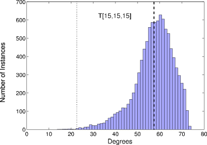
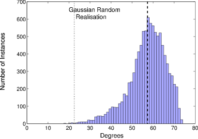
Figure 2: The full distribution of $\hat{\theta}$ for three T$[15,15,X]$ topologies, $X=15,4,1$, and for a Gaussian random realization. The dashed line shows the mean value and the dotted line the observed value. Note the extended low-end tail of the T[15,15,1] distribution, corresponding to the increased probability of this topology being able to produce the observed result.

Although the shift of the ensemble mean is small, topology might nevertheless help explain the observation if it alters the distribution of $\hat{\theta}$ for small angles. Figure 2 shows the full distribution of mean angle $\hat{\theta}$ obtained from 10,000 realizations of the corresponding topologies. Such a large number of simulations was used in order to trace the tails of the distribution accurately. The value of one radian, which is the expected mean angle for a Gaussian random realization, is shown with a thick dashed line, and the observed value is shown as a dotted line. While the distribution of $\hat{\theta}$ extends a little towards smaller values as the size of the smaller dimension of the toroid decreases, the observed value remains significantly low even for the smallest dimension considered.

We quantify this further in Figure 3, which shows the fraction of the ensemble giving a value at least as low as the observed one. The uncertainties are estimated using the Poisson error on the number of such ensemble members. We confirm the result of LM that approximately 0.1% of Gaussian skies give the observed value or lower. For small topology scales we see an enhancement in this fraction, but even for the smallest topology considered, the probability remains below one percent. We conclude that the observed alignment is not predicted by slab-space topologies.

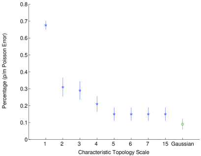
Figure 3: The fraction of realizations of a given T$[15,15,X]$ topology which provide a result at least as low as the observed result ($\hat{\theta}=22.5^{\circ}$), shown as a function of the characteristic topology scale $X$.

We have only asked whether the topologies within our set can explain the result found by LM. This is not achieved even by the smallest topologies we consider. However we note further that such small topologies are almost certainly already excluded by other observations OSS . For instance, a harmonic space analysis of precisely these same simulated topologies Kunz2005a suggests that $X<3$ is excluded by comparison to WMAP data (see also Ref. PK ). Such topologies are also constrained by the null results of matched circles tests for such topologies CDS ; starkman , corresponding to a limit of about $X\sim 5$. [The very tentative indications of dodecahedral topology found in Ref. Lum are interesting but of no significance for the topologies we consider here.] We have found that such topologies also do not receive any real support even from the observed alignments of the type discussed here.

III.3 The Land–Magueijo statistic for ILC simulations

Stepping somewhat aside from the main drive of this paper, we have made a small study of foreground effects by finding the distribution of $\hat{\theta}$ that results from the 10000 ILC simulations provided by Eriksen et al. Eriksen2005 . These simulations additionally (over an assumed Gaussian CMB sky) contain the residual level of foregrounds that can be expected from the ILC method of foreground subtraction. The distribution of $\hat{\theta}$ that results is much broader and flatter towards smaller angles. That is expected because the simulations contain residuals of the galaxy, so that a preferred axis going through the galactic poles or thereabouts will be expected for the lower $\ell$ and hence $\hat{\theta}$ will be smaller.

This result does not, however, explain the Land–Magueijo result, as the alignment they find (which is identified in the TOH maps) is not directed towards the galactic poles. It seems that if there were a preferred axis in a Gaussian CMB sky contaminated by galactic residuals, then it would be in the direction of the poles. This agrees with the conclusion of Copi et al. CHSS that the alignments seen do not correlate with known foregrounds. Also, note that the real ILC maps do not show the same alignment direction effect, the effect being spoilt due to the previously-mentioned presence of a near double maxima in one of the four multipoles considered.

To summarize, foreground contamination could explain a small $\hat{\theta}$ about the poles, but the observed orientation is not explained. Further, the alignment effect is detected in maps using a different foreground cleaning method TDH . Hence this may be a case where a curious real feature is being obscured by the presence of galactic contamination (and cosmic variance). Interestingly, this point has already be made for related alignment statistics by Slosar and Seljak SS .

IV Conclusions

Our main results are as follows. We have confirmed the observed value of $\hat{\theta}$ found by Land and Magueijo, while noting that it is quite dependent on the choice of maps used. We have also confirmed their result that Gaussian skies have only about 0.1% chance of finding a value as low as that observed in the TOH maps. By analyzing a set of slab-topology maps, we have found that there is a slightly-enhanced probability of such a low value being obtained, but in absolute terms it remains extremely unlikely. We conclude that slab topology is not the explanation for the multipole alignment found by Land and Magueijo. The resolution must lie elsewhere, perhaps in other topologies, or instead in other cosmological assumptions, or in foreground or instrumental noise.

References

- (1) M. Tegmark, A. de Oliveira-Costa, and A. J. S. Hamilton, Phys. Rev. D68, 123523 (2003), astro-ph/0302496.
- (2) A. de Oliveira-Costa, M. Tegmark, M. Zaldarriaga, and A. Hamilton, Phys. Rev. D69, 063516 (2004), astro-ph/0307282.
- (3) H. K. Eriksen, F. K. Hansen, A. J. Banday, K. M. Gorski, and P. B. Lilje, Astrophys. J. 605, 14 (2004), Erratum-ibid. 609, 1198 (2004), astro-ph/0307507.
- (4) H. K. Eriksen, A. J. Banday, K. M. Gorski, and P. B. Lilje, Astrophys. J. 612, 633, (2004), astro-ph/0403098.
- (5) F. K. Hansen, P. Cabella, D. Marinucci, and N. Vittorio, Astrophys. J. 607, L67 (2004), astro-ph/0402396; F. K. Hansen, A. J. Banday, and K. M. Gorski, astro-ph/0404206.
- (6) P. Bielewicz, K. M. Gorski, and A. J. Banday, Mon. Not. Roy. Astron. Soc. 355, 1283 (2004), astro-ph/0405007.
- (7) K. Land and J. Magueijo, Phys. Rev. Lett. 95, 071301 (2005), astro-ph/0502237.
- (8) C. J. Copi, D. Huterer, D. J. Schwarz, and G. D. Starkman, astro-ph/0508047.
- (9) A. Bernui, B. Mota, M. J. Rebouças, and R. Tavakol, astro-ph/0511666.
- (10) M. Lachieze-Rey and J.-P. Luminet, Phys. Rep. 254, 135 (1995), gr-qc/9605010; J. Levin, Phys. Rep. 365, 251 (2001), gr-qc/0108043; G. McCabe, Studies in the History and Philosophy of Modern Physics, 35, 549 (2004), gr-qc/0503028; M. J. Rebouças, AIP Conference Proceedings 782, 188, AIP, Melville, NY (2005), astro-ph/0504365; W. J. Hipólito-Ricald and G. I. Gomero, astro-ph/0507238.
- (11) A. Riazuelo, J.-P. Uzan, R. Lehoucq, and J. Weeks, Phys. Rev. D69, 103514 (2004), astro-ph/0212223.
- (12) A. Riazuelo, J. Weeks, J.-P. Uzan, R. Lehoucq, and J.-P. Luminet, Phys. Rev. D69, 103518 (2004), astro-ph/0311314.
- (13) W. Hu and M. White, Phys. Rev. D56, 596 (1997), astro-ph/9702170.
- (14) N. J. Cornish, D. Spergel, and G. Starkman, Class. Quant. Grav. 15, 2657 (1998), astro-ph/9801212.
- (15) M. Kunz, N Aghanim, L. Cayon, O. Forni, A. Riazuelo, and J.-P. Uzan, astro-ph/0510164.
- (16) N. J. Cornish, D. N. Spergel, G. D. Starkman, and E. Komatsu, Phys. Rev. Lett. 92, 201302 (2004), astro-ph/0310233.
- (17) C. L. Bennett et al. (WMAP collaboration), Astrophys. J. Suppl. 148, 97 (2003), astro-ph/0302208.
- (18) P. Bielewicz, H. K. Eriksen, A. J. Banday, K. M. Gorski, and P. B. Lilje, astro-ph/0507186.
- (19) C. Vale, astro-ph/0509039.
- (20) J. Medeiros and C. R. Contaldi, astro-ph/0510816.
- (21) P. Coles, P. Dineen, J. Earl, and D. Wright, Mon. Not. Roy. Astron. Soc. 350, 989 (2004), astro-ph/0310252.
- (22) A. de Oliveira-Costa, G. F. Smoot, and A. A. Starobinsky, Astrophys. J. 468, 457 (1996), astro-ph/9510109.
- (23) N. G. Phillips and A. Kogut, astro-ph/0404400.
- (24) J.-P. Luminet, J. Weeks, A. Riazuelo, R. Lehoucq, and J.-P. Uzan, Nature 425, 593 (2003), astro-ph/0310253; B. F. Roukema, B. Lew, M. Cechowska, A. Marecki, and S. Bajtlik, Astron. Astrophys. 423, 821 (2004), astro-ph/0402608; R. Aurich, S. Lustig, and F. Steiner, astro-ph/0510847.
- (25) H. K. Eriksen, A. J. Banday, K. M. Gorski, and P. B. Lilje, astro-ph/0508196.
- (26) A. Slosar and U. Seljak, Phys. Rev. D70, 083002 (2004), astro-ph/0404567.
- (27) K. M. Gorski, E. Hivon, A. J. Banday, B. D. Wandelt, F. K. Hansen, M. Reinecke, and M. Bartelman, Astrophys. J. 622, 759 (2005), astro-ph/0409513 [see also http://healpix.jpl.nasa.gov/].