The cosmic reionization history as revealed by the CMB Doppler–21-cm correlation

Abstract

We show that the epoch(s) of reionization when the average ionization fraction of the universe is about half can be determined by correlating Cosmic Microwave Background (CMB) temperature maps with 21-cm line maps at degree scales ($l\sim 100$). During reionization peculiar motion of free electrons induces the Doppler anisotropy of the CMB, while density fluctuations of neutral hydrogen induce the 21-cm line anisotropy. In our simplified model of inhomogeneous reionization, a positive correlation arises as the universe reionizes whereas a negative correlation arises as the universe recombines; thus, the sign of the correlation provides information on the reionization history which cannot be obtained by present means. The signal comes mainly from large scales ($k\sim 10^{-2}~{}{\rm Mpc}^{-1}$) where linear perturbation theory is still valid and complexity due to patchy reionization is averaged out. Since the Doppler signal comes from ionized regions and the 21-cm comes from neutral ones, the correlation has a well defined peak(s) in redshift when the average ionization fraction of the universe is about half. Furthermore, the cross-correlation is much less sensitive to systematic errors, especially foreground emission, than the auto-correlation of 21-cm lines: this is analogous to the temperature-polarization correlation of the CMB being more immune to systematic errors than the polarization-polarization. Therefore, we argue that the Doppler-21cm correlation provides a robust measurement of the 21-cm anisotropy, which can also be used as a diagnostic tool for detected signals in the 21-cm data — detection of the cross-correlation provides the strongest confirmation that the detected signal is of cosmological origin. We show that the Square Kilometer Array can easily measure the predicted correlation signal for 1 year of survey observation.

1. Introduction

When and how was the universe reionized? This question is deeply connected to the physics of formation and evolution of the first generations of ionizing sources (stars or quasars or both) and the physical conditions in the interstellar and the intergalactic media in a high redshift universe. This field has been developed mostly theoretically (Barkana & Loeb, 2001; Bromm & Larson, 2004; Ciardi & Ferrara, 2005; Iliev et al., 2005; Alvarez, Bromm, & Shapiro, 2005) because there are only a very limited number of observational probes of the epoch of reionization: the Gunn–Peterson test (Gunn & Peterson, 1965; Becker et al., 2001), polarization of the Cosmic Microwave Background (CMB) on large angular scales (Zaldarriaga, 1997; Kaplinghat et al., 2003; Kogut et al., 2003), mean intensity (Santos, Bromm, & Kamionkowski, 2002; Salvaterra & Ferrara, 2003; Cooray & Yoshida, 2004; Madau & Silk, 2005; Fernandez & Komatsu, 2005) and fluctuations (Magliocchetti, Salvaterra, & Ferrara, 2003; Kashlinsky et al., 2004; Cooray et al., 2004; Kashlinsky et al., 2005) of the near infrared background from redshifted UV photons, Ly$\alpha$-emitters at high redshift (Malhotra & Rhoads, 2004; Santos, 2004; Furlanetto, Hernquist, & Zaldarriaga, 2004; Haiman & Cen, 2005; Wyithe & Loeb, 2005) and fluctuations of the 21-cm line background from neutral hydrogen atoms during reionization (Ciardi & Madau, 2003; Furlanetto, Sokasian, & Hernquist, 2004; Zaldarriaga, Furlanetto, & Hernquist, 2004) or even prior to reionization (Scott & Rees, 1990; Madau, Meiksin, & Rees, 1997; Tozzi et al., 2000; Iliev et al., 2002; Shapiro et al., 2005).

Each one of these methods probes different epochs and aspects of cosmic reionization: the Gunn–Peterson test is sensitive to a very small amount of residual neutral hydrogen present at the late stages of reionization ($z\sim 6$), Ly$\alpha$-emitting galaxies and the wavelengths of the near infrared background probe the intermediate stages of reionization ($7\lesssim z\lesssim 15$), the 21-cm background probes the earlier stages where the majority of the intergalactic medium is still neutral ($10\lesssim z\lesssim 30$), and the CMB polarization measures the column density of free electrons integrated over a broader redshift range ($z\lesssim 20$, say). Since different datasets are complementary, one expects that cross-correlations between them add more information than can be obtained by each dataset alone. For example, the information content in the CMB and the 21-cm background cannot be exploited fully until the cross-correlation is studied: if we just extract the power spectrum from each dataset, we do not exhaust the information content in the whole dataset because we are ignoring the cross-correlation between the two. The cross-correlation always reveals more information than can be obtained from the datasets individually unless the two are perfectly correlated (and Gaussian) or totally uncorrelated.

Motivated by these considerations, we study the cross-correlation between the CMB temperature anisotropy and the 21-cm background on large scales. We show that the CMB anisotropy from the Doppler effect and the 21-cm line background can be anti-correlated or correlated at degree scales ($l\sim 100$), and both the amplitude and the sign of the correlation tell us how rapidly the universe reionized or recombined, and locations of the correlation (or the anti-correlation) peak(s) in redshift space tell us when reionization or recombination happened. This information is difficult to extract from either the CMB or the 21-cm data alone. Our work is different from recent work on a similar subject by Salvaterra et al. (2005). While they studied a similar cross-correlation on very small scales ($\sim$ arc-minutes), we focus on much larger scales ($\sim$ degrees) where matter fluctuations are still linear and complexity due to patchy reionization is averaged out. Cooray (2004) studied higher-order correlations such as the bispectrum on arc-minute scales. For our case, however, fluctuations are expected to follow nearly Gaussian statistics on large scales, and thus one cannot obtain more information from higher-order statistics. He also studied the cross-correlation power spectrum of the CMB and projected 21-cm maps, and concluded that the signal would be too small to be detectable owing to the line-of-sight cancellation of the Doppler signal in the CMB. However, we show that cancellation can be partially avoided by cross-correlating the CMB map with 21-cm maps at different redshifts (tomography). Prospects for the Square Kilometer Array (SKA) to measure the cross-correlation signal on degree scales are shown to be promising.

Throughout the paper, we use $c=1$ and the following convention for the Fourier transformation:

$$f(\hat{\mathbf{n}},\eta)=\int\frac{d^{3}{\mathbf{k}}}{(2\pi)^{3}}f_{\mathbf{k}}e^{-i{\mathbf{k}}\cdot{\hat{\mathbf{n}}}(\eta_{0}-\eta)},$$ (1)

where $\hat{\mathbf{n}}$ is the directional cosine along the line of sight pointing toward the celestial sphere, $\eta$ is the conformal time, $\eta(z)=\int_{0}^{t}dt^{\prime}/a(t^{\prime})=\int_{z}^{\infty}dz^{\prime}/H(z^{\prime})$, and $\eta_{0}$ is the conformal time at present. Note that

$$\eta_{0}-\eta(z)=\int_{0}^{z}\frac{dz^{\prime}}{H(z^{\prime})},$$ (2)

which equals the comoving distance, $r(z)=\eta_{0}-\eta(z)$, in flat geometry (with $c=1$). Also, using Rayleigh’s formula one obtains

$$f(\hat{\mathbf{n}},\eta)=4\pi\sum_{lm}(-i)^{l}\int\frac{d^{3}{\mathbf{k}}}{(2\pi)^{3}}f_{\mathbf{k}}j_{l}[k(\eta_{0}-\eta)]Y_{lm}(\hat{\mathbf{n}})Y_{lm}^{*}(\hat{\mathbf{k}}).$$ (3)

The cosmological parameters are fixed at $\Omega_{m}=0.3$, $\Omega_{b}=0.046$, $\Omega_{\Lambda}=0.7$, $h=0.7$, and $\sigma_{8}=0.85$, and we assume a scale invariant initial power spectrum for matter perturbations.

This paper is organized as follows. In § 2 and 3 we derive the analytic formula for the Doppler–21-cm correlation power spectrum. Equations (15) or (24) are the main result. We then present a physical picture of the correlation and describe properties of the correlation in detail. We also discuss the validity of our assumptions and possible effects of more realistic reionization scenarios. In § 4 we discuss detectability of the correlation signal with SKA before concluding in § 5.

2. 21-cm Fluctuations and CMB Doppler Anisotropy

2.1. 21-cm Signal

Following the notation of Zaldarriaga, Furlanetto, & Hernquist (2004), we write the observed differential brightness temperature of the 21-cm emission line at $\lambda=21~{}{\rm cm}(1+z)$ in the direction of $\hat{\mathbf{n}}$ as

$$T_{21}(\hat{\mathbf{n}},z)=T_{0}(z)\int_{0}^{\eta_{0}}d\eta^{\prime}W[\eta(z)-\eta^{\prime}]\psi_{21}(\hat{\mathbf{n}},\eta^{\prime}),$$ (4)

where $W(\eta(z)-\eta^{\prime})$ is a normalized ($\int_{-\infty}^{\infty}dxW(x)=1$) spectral response function of an instrument which is centered at $\eta(z)-\eta^{\prime}=0$, $T_{0}(z)$ is a normalization factor given by

$$T_{0}(z)\simeq 23~{}{\rm mK}~{}\left(\frac{\Omega_{b}h^{2}}{0.02}\right)\left[\left(\frac{0.15}{\Omega_{m}h^{2}}\right)\left(\frac{1+z}{10}\right)\right]^{1/2},$$ (5)

and

$$\psi_{21}(\hat{\mathbf{n}},\eta)\equiv x_{H}(\hat{\mathbf{n}},\eta)[1+\delta_{b}(\hat{\mathbf{n}},\eta)]\left[1-\frac{T_{\rm cmb}(\eta)}{T_{\rm s}(\hat{\mathbf{n}},\eta)}\right]\rightarrow\left\{1-{\overline{x}_{e}}(\eta)[1+\delta_{x}(\hat{\mathbf{n}},\eta)]\right\}\left\{1+\delta_{b}(\hat{\mathbf{n}},\eta)\right\},$$ (6)

where $\delta_{b}$ is the baryon density contrast,

$$\delta_{x}\equiv\frac{x_{e}-{\overline{x}_{e}}}{\overline{x}_{e}},$$ (7)

is the ionized fraction contrast, $x_{H}$ is the neutral fraction, and $x_{e}\equiv 1-x_{H}$ is the ionized fraction. Here, we have assumed that the spin temperature of neutral hydrogen, $T_{\rm s}$, is much larger than the CMB temperature, $T_{\rm cmb}$. This assumption is valid soon after reionization begins (Ciardi & Madau, 2003).

To simplify the calculation, we assume that the spectral resolution of the instrument is much smaller than the features of the target signal in redshift space. This is always a very good approximation. (For the effect of a relatively large bandwidth, see Zaldarriaga, Furlanetto, & Hernquist (2004).) Therefore, we set $W(x)=\delta^{D}(x)$ to obtain $T_{21}(\hat{\mathbf{n}},z)=T_{0}(z)\psi_{21}[\hat{\mathbf{n}},\eta(z)]$. To leading order in $\delta_{x}$ and $\delta_{b}$, the spherical harmonic transform of $T_{21}(\hat{\mathbf{n}},z)$ is given by

$$a_{lm}^{21}(z)=4\pi(-i)^{l}\int\frac{d^{3}k}{(2\pi)^{3}}[\overline{x}_{H}(z)(1+f\mu^{2}){{\delta}}_{b\bf{k}}-{\overline{x}_{e}}(z){{\delta}}_{x\bf{k}}]\alpha_{l}^{21}(k,z)Y_{lm}^{*}({\bf{k}}),$$ (8)

where $\alpha^{21}_{l}(k,z)$ is a transfer function for the 21-cm line,

$$\alpha^{21}_{l}(k,z)\equiv T_{0}(z)D(z)j_{l}[k(\eta_{0}-\eta)],$$ (9)

$D(z)$ is the growth factor of linear perturbations, $\mu\equiv\hat{\mathbf{k}}\cdot\hat{\mathbf{n}}$, and $f\equiv d\ln D/d\ln a$. The factor $(1+f\mu^{2})$ takes account of the enhancement of the fluctuation amplitude due to the redshift-space distortion, the so-called “Kaiser effect” (Kaiser 1987; see also Bharadwaj & Ali 2004 and Barkana & Loeb 2005).

2.2. Doppler Signal

The CMB temperature anisotropy from the Doppler effect is given by

$$T_{D}({\bf\hat{n}})=-T_{\rm cmb}\int_{0}^{\eta_{0}}d\eta\dot{\tau}e^{-\tau}{\bf\hat{n}}\cdot{\bf v}_{b}({\bf\hat{n}},\eta)=-T_{\rm cmb}\int_{0}^{\eta_{0}}d\eta\dot{\tau}e^{-\tau}{\bf\hat{n}}\cdot\int\frac{d^{3}k}{(2\pi)^{3}}{{\mathbf{v}}_{b{\mathbf{k}}}}(\eta)e^{-i{\bf k}\cdot{\bf\hat{n}}(\eta_{0}-\eta)},$$ (10)

where $T_{\rm cmb}=2.725~{}K$ is the present-day CMB temperature, $\dot{x}\equiv\partial x/\partial\eta$, $\tau(\eta)\equiv\sigma_{T}\int_{0}^{\eta}d\eta^{\prime}n_{e}(\eta^{\prime})$ is the Thomson scattering optical depth, and ${{\mathbf{v}}_{b{\mathbf{k}}}}$ is the peculiar velocity of baryons. In deriving the above formula, we have neglected the fluctuation of ionized fraction, $\delta_{x}(\hat{\mathbf{n}},\eta)$, and electron number density, $\delta_{e}(\hat{\mathbf{n}},\eta)$, since their contributions to the cross-correlation would be higher order corrections (the effect due to $\delta_{e}{\mathbf{v}}_{b}$ is called the Ostriker–Vishniac effect; e.g., Ostriker & Vishniac 1986), and such a correction is negligible for linear fluctuations on the large scales we consider here. Note that the negative sign ensures that we see a blueshift, $T_{D}(\hat{\mathbf{n}})>0$, when baryons are moving toward us, $\hat{\mathbf{n}}\cdot{\mathbf{v}}_{b}<0$. The peculiar velocity is related to the density contrast via the continuity equation for baryons, ${{\mathbf{v}}_{b{\mathbf{k}}}}=-i({\bf k}/{k^{2}})\delta_{b\bf k}\dot{D}$. One obtains

$$T_{D}({\bf\hat{n}})=T_{\rm cmb}\int_{0}^{\eta_{0}}d\eta\dot{D}\dot{\tau}e^{-\tau}\int\frac{d^{3}k}{(2\pi)^{3}}\frac{\delta_{b\bf k}}{k^{2}}\frac{\partial}{\partial\eta}e^{-i{{\bf k\cdot\hat{n}}(\eta_{0}-\eta)}}.$$ (11)

The spherical harmonic transform of $T_{D}(\hat{\mathbf{n}},z)$ is then given by

$$a^{D}_{lm}=4\pi(-i)^{l}\int\frac{d^{3}k}{(2\pi)^{3}}{{\delta}}_{b\bf{k}}\alpha^{D}_{l}(k)Y_{lm}^{*}({\bf{k}}),$$ (12)

where $\alpha^{D}_{l}(k)$ is a transfer function for the Doppler effect,

$$\alpha^{D}_{l}(k)\equiv\frac{T_{\rm cmb}}{k^{2}}\int_{0}^{\eta_{0}}d\eta\dot{D}\dot{\tau}e^{-\tau}\frac{\partial}{\partial\eta}j_{l}[k(\eta_{0}-\eta)].$$ (13)

3. Doppler–21-cm Correlation

3.1. Generic Formula

Given the spherical harmonic coefficients just derived for the 21-cm line (Eq. [8]) and the Doppler anisotropy (Eq. [12]), one can calculate the cross-correlation power spectrum, $C_{l}^{21-D}$, exactly as

$$C^{21-D}_{l}(z)$$

$$= \langle a^{21}_{lm}(z)a^{D*}_{lm}\rangle=\frac{2}{\pi}\int_{0}^{\infty}k^{2}dk\left[\overline{x}_{H}(z)(1+f\langle\mu^{2}\rangle)P_{\delta\delta}(k)-\overline{x}_{e}(z)P_{x\delta}(k)\right]\alpha_{l}^{21}(k,z)\alpha_{l}^{D}(k)$$

$$= T_{\rm cmb}T_{0}(z)D(z)\frac{2}{3\pi}\int_{0}^{\infty}dk\left[4\overline{x}_{H}(z)P_{\delta\delta}(k)-3\overline{x}_{e}(z)P_{x\delta}(k)\right]j_{l}[k(\eta_{0}-\eta)]\int_{0}^{\eta_{0}}d\eta^{\prime}\dot{D}\dot{\tau}e^{-\tau}\frac{\partial}{\partial\eta^{\prime}}j_{l}[k(\eta_{0}-\eta^{\prime})],$$

where we have defined the matter power spectrum, $P_{\delta\delta}(k)$, as $\langle\delta_{\bf k}\delta^{*}_{{\bf k}^{\prime}}\rangle\equiv(2\pi)^{3}\delta({\bf k}-{\bf k}^{\prime})P_{\delta\delta}(k)$, and the cross-correlation power spectrum between ionized fraction and density $P_{x\delta}(k)$, as $\langle\delta_{x\bf k}\delta^{*}_{{\bf k}^{\prime}}\rangle\equiv(2\pi)^{3}\delta({\bf k}-{\bf k}^{\prime})P_{x\delta}(k)$. In the last line of equation (3.1), we have used $f\langle\mu^{2}\rangle=1/3$ for a matter-dominated universe. Note that $\delta$ used in these power spectra is the density contrast of total matter, $\delta$, as baryons trace total matter perturbations, $\delta_{b}=\delta$, on the scales of our interest (scales much larger than the Jeans length of baryons). Equation (3.1) can be simplified by integrating it by parts:

$$C^{21-D}_{l}(z) = -T_{\rm cmb}T_{0}(z)D(z)\frac{2}{3\pi}\int_{0}^{\eta_{0}}d\eta^{\prime}\frac{\partial}{\partial\eta^{\prime}}\dot{D}\dot{\tau}e^{-\tau}$$ (15)

$$\times \int_{0}^{\infty}dk\left[4\overline{x}_{H}(z)P_{\delta\delta}(k)-3\overline{x}_{e}(z)P_{x\delta}(k)\right]j_{l}[k(\eta_{0}-\eta)]j_{l}[k(\eta_{0}-\eta^{\prime})].$$

A further simplification can be made by using an approximation to the integral of the product of spherical Bessel functions for $l\gg 1$:

$$\frac{2}{\pi}\int_{0}^{\infty}dkP(k)j_{l}(kr)j_{l}(kr^{\prime})\approx P\left(k=\frac{l}{r}\right)\frac{\delta(r-r^{\prime})}{l^{2}},$$ (16)

where $r(z)=\eta_{0}-\eta(z)$ is the comoving distance out to an object at a given $z$. We obtain

$$l^{2}C_{l}^{21-D}(z)\approx-T_{\rm cmb}T_{0}(z)D(z)\left[\frac{4}{3}\overline{x}_{H}(z)P_{\delta\delta}\left(\frac{l}{r(z)}\right)-\overline{x}_{e}(z)P_{x\delta}\left(\frac{l}{r(z)}\right)\right]\frac{\partial}{\partial\eta}(\dot{D}\dot{\tau}e^{-\tau}).$$ (17)

In what follows we will use the exact expression given by equation (15) in our main quantitative results, while we will retain the approximate expression given by equation (17) to develop a more intuitive understanding of the origin of the cross-correlation. We have found that the exact expression gives results which are about 10% lower (at $l\sim 100$) than the approximate expression of equation (17) for the single reionization history we will use in § 3.4, while for the double reionization history the exact result is smaller by about 40%. This is because the line-of-sight integral in equation (3.1) acts to smooth out features in redshift, an effect which dissappears when the delta function is used in the approximation. Since the double reionization model fluctuates much more strongly in redshift than the single reionization model, the effect is more apparent for double reionization.

Equation (17) implies one important fact: the cross-correlation vanishes if $\dot{D}\dot{\tau}e^{-\tau}$ is constant. In other words, the amplitude of the signal directly depends on how rapidly structure grows and reionization proceeds, and the sign of the correlation depends on the direction of reionization (whether the universe recombines or reionizes). Moreover, the shape of $l^{2}C_{l}(z)$ directly traces the shape of the matter power spectrum at $k=l/r(z)$. It is well known that $P(k)$ has a broad peak at the scale of the horizon size at the epoch of matter-radiation equality, $k_{\rm eq}\simeq 0.011~{}{\rm Mpc}^{-1}~{}(\Omega_{m}h^{2}/0.15)$. Since the conformal distance (which is the same as the comoving angular diameter distance in flat geometry) is on the order of $10^{4}$ Mpc at high redshifts, the correlation power spectrum will have a peak at degree scales, $l\sim 10^{2}$.

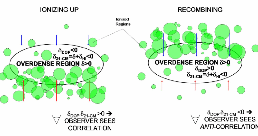
Figure 1.— Simplified schematic diagram illustrating the nature of the correlation between the Doppler and 21-cm anisotropies. Red arrows pointing away from the observer indicate ionized gas falling into the positive density perturbation (represented by the black oval) from the near side, whereas blue arrows represent ionized gas falling in from the far side. During reionization, there is more ionized gas on the near side of the perturbation (at lower redshift) than on the far side. This implies that the net effect from this perturbation is a redshift of the CMB in that direction (labeled as $\delta_{\rm DOP}<0$). Because the sources responsible for reionization are located in halos which are very biased relative to the underlying linear density field, the overdense region shown here is actually underdense in neutral hydrogen, so that this overdensity represents a negative fluctuation in the 21-cm signal (labeled as $\delta_{\rm 21-cm}<0$). Because both the 21-cm and the Doppler fluctuations from a region that is undergoing reionization are both the same sign, the signature of reionization is a positive correlation, while recombination (in which the situation is reversed for the Doppler signal) results in an anti-correlation. In reality, the growth of fluctuations and the dependence of the density on redshift complicate the picture, so that the sign of the signal is determined not by the derivative of the ionized fraction $d[x_{e}]/dz$, but rather $d[x_{e}(z)(1+z)^{3/2}]/dz$ (see equation 23).

3.2. Ionized Fraction–Density Correlation

While $P_{\delta\delta}(k)$ is a known function on the scales of interest here, the cross-correlation between ionized fraction and density, $P_{x\delta}(k)$, is not. In order to understand its importance in determining the observable signal, we have estimated its value on large scales. Since we give the full details of derivations in Appendix, we quote only the result here:

$$\overline{x}_{e}(z)P_{x\delta}(k)=-\overline{x}_{H}(z)\ln\overline{x}_{H}(z)\left[{\overline{b}}_{h}(z)-1-f\right]P_{\delta\delta}(k),$$ (18)

where $\overline{b}_{h}(z)$ is the average bias of dark matter halos more massive than $m_{\rm min}$,

$${\overline{b}_{h}}(z)=1+\sqrt{\frac{2}{\pi}}\frac{e^{-\delta_{c}^{2}(z)/2\sigma_{\rm min}^{2}}}{f_{\rm coll}(z)D(z)\sigma_{\rm min}},$$ (19)

$m_{\rm min}$ is the minimum halo mass capable of hosting ionizing sources, $f_{\rm coll}(z)$ is the fraction of matter in the universe collapsed into halos with $m>m_{\rm min}$, and $\sigma_{\rm min}\equiv\sigma(m_{\rm min})$ is the r.m.s. of density fluctuations at the scale of $m_{\rm min}$ at $z=0$. We take $m_{\rm min}$ to be the mass of a halo with a virial temperature $T_{\rm min}$, which we will treat as a free parameter. Here, $f$ is a parameter characterizing the physics of reionization: $f=0$ is the “photon counting limit”, in which recombinations are not important in determining the extent of ionized regions. On the other hand, $f=1$ is the “Strömgren limit”, in which the ionization rate is balanced by the recombination rate, as would occur in a Strömgren sphere. While our choice for the range of $f$ is resonable, larger values are possible if recombinations limit the size of H II regions and the clumping factor increases with increasing density. Equation (19) is general in the sense that it can accomodate such a scenario. It is easy to check that $P_{x\delta}$ naturally satisfies the physical constraints: it vanishes when the universe is either fully neutral, $\overline{x}_{H}=1$, or fully ionized, $\overline{x}_{H}=0$. Although we have derived an explicit relationship between $P_{x\delta}$ and $P_{\delta\delta}$ (which is based on several simplifying assumptions – see Appendix), we note that the formulae presented here are sufficiently flexible so that any model for the large-scale bias of reionization with $P_{x\delta}=b_{x\delta}P_{\delta\delta}$ can be substituted for the one we use here.

We simplify equations (3.1) and (17) by making the approximations that $e^{-\tau}\approx 1$ (justified by observations of the CMB polarization; see Kogut et al. 2003) and

$$D(z)=\frac{1+z_{N}}{1+z},$$ (20)

which is a very good approximation at $z\gg 1$ when the universe is still matter-dominated. The linear growth factor has been normalized such that $D(z_{N})=1$; thus,

$$\dot{D}=-H(z)\frac{d}{dz}\frac{1+z_{N}}{1+z}=\frac{(\Omega_{m}H_{0}^{2})^{1/2}(1+z_{N})}{(1+z)^{1/2}}.$$ (21)

We also use the relation

$$\dot{\tau}(z) = \sigma_{T}\frac{\rho_{b0}}{m_{p}}(1-Y_{p})(1+z)^{2}{\overline{x}_{e}}(z)$$ (22)

$$= 0.0525H_{0}\Omega_{b}h(1+z)^{2}\overline{x}_{e}(z),$$

where $\rho_{b0}$ is the baryon density at present, $Y_{p}=0.24$ is the helium mass abundance (hydrogen ionization only is assumed), and ${\overline{x}_{e}}(z)$ is the ionized fraction. One finds

$$\frac{\partial}{\partial\eta}(\dot{D}\dot{\tau}e^{-\tau})=-0.0525H_{0}^{3}\Omega_{m}\Omega_{b}h(1+z_{\rm N})(1+z)^{3/2}\frac{d}{dz}\left[{\overline{x}_{e}}(z)(1+z)^{3/2}\right].$$ (23)

Combining equations (3.1) and (23), we obtain

$$\frac{l^{2}C^{21-D}_{l}(z)}{2\pi} = 0.37~{}\mu{\rm K}^{2}~{}\left(\frac{\Omega_{b}h^{2}}{0.02}\right)^{2}\left(\frac{\Omega_{m}h^{2}}{0.15}\right)^{1/2}{\overline{x}}_{H}(z)\left[4/3+\ln{\overline{x}}_{H}(z)\left({\overline{b}}_{h}-f-1\right)\right]$$ (24)

$$\times \left(\frac{1+z}{10}\right)^{-1/2}\int_{0}^{\infty}dz^{\prime}\frac{F_{l}(z,z^{\prime})}{H(z^{\prime})}(1+z^{\prime})^{3/2}\frac{d}{dz^{\prime}}\left[{\overline{x}_{e}}(z^{\prime})(1+z^{\prime})^{3/2}\right],$$

where

$$F_{l}(z,z^{\prime})=l^{2}\int_{0}^{\infty}dk\frac{P(k)(1+z_{N})^{2}}{10^{5}{\rm Mpc}^{3}}j_{l}\left[k(\eta_{0}-\eta(z))\right]j_{l}\left[k(\eta_{0}-\eta(z^{\prime}))\right].$$ (25)

The approximation of equation (17) and equation (23) imply

$$\frac{l^{2}C^{21-D}_{l}(z)}{2\pi} \simeq 18.4~{}\mu{\rm K}^{2}~{}\left(\frac{\Omega_{b}h^{2}}{0.02}\right)^{2}\left(\frac{\Omega_{m}h^{2}}{0.15}\right)^{1/2}{\overline{x}}_{H}(z)\left[4/3+\ln{\overline{x}}_{H}(z)\left({\overline{b}}_{h}-f-1\right)\right]$$ (26)

$$\times \frac{P_{\delta\delta}[l/r(z),z_{N}](1+z_{N})^{2}}{10^{5}~{}{\rm Mpc}^{3}}\frac{d}{dz}\left[{\overline{x}_{e}}(z)(1+z)^{3/2}\right]\left(\frac{1+z}{10}\right).$$

Note that $P(k,z_{N})(1+z_{N})^{2}$ is independent of the normalization epoch, $z_{N}$, for $z_{N}\gg 1$; the result is independent of the choice of $z_{N}$, as expected. These equations are the main result of this paper, and we shall use these results to investigate the properties of the correlation in more detail. Since we have a product of $d\overline{x}_{e}/dz$ and $\overline{x}_{H}$, we expect that the largest contribution comes from the “epoch of reionization” when $\overline{x}_{e}(z)$ changes most rapidly. Therefore, by detecting the Doppler–21-cm correlation peak(s), one can determine the epoch(s) of reionization. The sign of the cross-correlation is also very important. The sign of the cross-correlation is determined by the sign of the derivative term and the difference between ${\overline{x}}_{H}P_{\delta\delta}$ and ${\overline{x}}_{e}P_{x\delta}$. For the case in which ${\overline{x}}_{H}P_{\delta\delta}>{\overline{x}}_{e}P_{x\delta}$, the Doppler effect and the 21-cm emission are anti-correlated when the ionized fraction, $\overline{x}_{e}(z)$, increases toward low $z$ faster than $(1+z)^{-3/2}$. For our simplified model of inhomogeneous reionization (see Appendix), we find that ${\overline{x}}_{H}P_{\delta\delta}<{\overline{x}}_{e}P_{x\delta}$, however, and in this case we find a positive correlation as the universe is being reionized. This is unique information that cannot be obtained by present means. See Fig. 1 for a schematic diagram which describes the nature of the cross-correlation.

3.3. Illustration: Homogeneous Reionization Limit

It may be instructive to study the nature of the signal by taking the “homogeneous reionization limit”, in which the ionized fraction is uniform, $\delta_{x}\equiv 0$. Such a situation may be more relevant than our model for biased reionization if, for example, the photons responsible for reionization have a very long mean free path or clumping in denser regions cancels the effect of bias. In the homogeneous limit, the approximate formula (eq. 26) implies

$$\frac{l^{2}C^{21-D}_{l}(z)}{2\pi} \simeq 24.5~{}\mu{\rm K}^{2}~{}\left(\frac{\Omega_{b}h^{2}}{0.02}\right)^{2}\left(\frac{\Omega_{m}h^{2}}{0.15}\right)^{1/2}\frac{P_{\delta\delta}[l/r(z),z_{N}](1+z_{N})^{2}}{10^{5}~{}{\rm Mpc}^{3}}$$ (27)

$$\times {\overline{x}}_{H}(z)\frac{d}{dz}\left[{\overline{x}_{e}}(z)(1+z)^{3/2}\right]\left(\frac{1+z}{10}\right).$$

Figure 2.— (Left) Power spectrum of the cross-correlation between the cosmic microwave background anisotropy and the 21-cm line fluctuations, $l^{2}C_{l}^{21-D}/(2\pi)$. We assume $z=15$ for a reionization history given by equation (28) with a reionization redshift of $z_{r}=15$ and duration of $\Delta z=0.5$. Note that its shape follows that of the linear matter power spectrum, $P_{\delta\delta}(k)$ with $k\simeq l/r(z)$, where $r(z)$ is the comoving angular diameter distance. (Right) Evolution of the peak amplitude of $l^{2}C_{l}^{21-D}/(2\pi)$ at $l\sim 100$ from a homogeneous reionization history described by equation (28), for $\Delta z=0.5$ and different reionization redshifts, $z_{r}=7,11,15$ and 19, from left to right.

One may estimate the amplitude of the signal at the epoch of reionization, $z=z_{r}$, using a duration of reionization at $z_{r}$, $\Delta z$ as follows (omitting factors of order unity):

$$\frac{l^{2}C^{21-D}_{l}(z_{r})}{2\pi}\simeq-\frac{195~{}\mu{\rm K}^{2}}{\Delta z}\frac{\overline{x}_{H}(z_{r}){\overline{x}_{e}}(z_{r})}{0.25}\left(\frac{1+z_{r}}{10}\right)^{5/2}.$$

The remarkable feature is that the predicted signal is rather large. For $z_{r}=15$ (which is consistent with early reionization suggested by Kogut et al. (2003)) and $\Delta z=1$, we predict $l^{2}C^{21-D}_{l}/(2\pi)\sim-600~{}\mu{\rm K^{2}}$ at $l\sim 10^{2}$. Under these assumptions, therefore, detection of the anti-correlation peak should not be too difficult, given that the Wilkinson Microwave Anisotropy Probe (WMAP) has already obtained an accurate CMB temperature map at $l\sim 10^{2}$ (Bennett et al., 2003). When any experiment for measuring the 21-cm background at degree scales becomes on-line, one should correlate the 21-cm data on degree scales with the WMAP temperature map to search for this peak. Note also that in the homogeneous reionization limit the sign is reversed, so that reionization results in an anti-correlation. The sign of the correlation therefore depends sensitively on the degree to which reionization is biased on large scales.

3.4. Reionization History

To calculate the actual cross-correlation power spectrum, we need to specify the evolution of the ionized fraction, $\overline{x}_{e}(z)$. Computing $\overline{x}_{e}(z)$ from first principles is admittedly very difficult, and this is one of the most challenging tasks in cosmology today. To illustrate how the cross-correlation power spectrum changes for different reionization scenarios, therefore, we explore two simple parameterizations of the reionization history.

In one case, we assume that the ionized fraction increases monotonically toward low $z$. We use the simple parameterization adopted by Zaldarriaga, Furlanetto, & Hernquist (2004):

$$\overline{x}_{H}(z)=\frac{1}{1+{\rm exp}\left[-(z-z_{r})/\Delta z\right]},$$ (28)

where $z_{r}$ is the “epoch of reionization” when $\overline{x}_{H}(z_{r})=1/2$ and $\Delta z$ corresponds to its duration. In this case, one obtains a fully analytic formula for the correlation power spectrum:

$$\frac{l^{2}C^{21-D}_{l}(z)}{2\pi} \simeq 58~{}\mu{\rm K}^{2}~{}\left[4/3+\ln{\overline{x}}_{H}(z)\left({\overline{b}}_{h}-f-1\right)\right]\frac{P[l/r(z),z_{N}](1+z_{N})^{2}}{10^{5}~{}{\rm Mpc}^{3}}\left(\frac{\Omega_{b}h^{2}}{0.02}\right)^{2}\left(\frac{\Omega_{m}h^{2}}{0.15}\right)^{1/2}$$ (29)

$$\times{\overline{x}}_{H}(z){\overline{x}}_{e}(z)\left[\frac{3}{2}-\frac{\overline{x}_{H}(z)(1+z)}{\Delta z}\right]\left(\frac{1+z}{10}\right)^{3/2}.$$

In the homogeneous reionization limit, $P_{x\delta}\equiv 0$, one gets $l^{2}C_{l}/(2\pi)\simeq-165~{}\mu{\rm K}^{2}$ for $z=9=z_{r}$ and $\Delta z=1/2$, and the amplitude of the signal scales as $(1+z_{r})^{5/2}$, as expected (see Eq. [3.3]). For an early reionization at $z_{r}=15$, the homogeneous reionization model predicts $l^{2}C_{l}/(2\pi)\simeq-570~{}\mu{\rm K}^{2}$.

Figure 3.— (top and left panels) Peak correlation amplitude vs. redshift. Each panel is labeled with a different value of $f$ which parameterizes the uncertainty in the physics of reionization (see Appendix for the definition of $f$ and detailed discussion). The most likely value of $f$ is somewhere between 0 and 1. The dotted line corresponds to the homogeneous reionization limit in which fluctuations in the ionized fraction are totally ignored (Eq. [27]), while the thick line takes into account fluctuations in the ionized fraction (Eq. [26]). The dashed line is the difference between the homogeneous reionization and the total signal. (bottom right) Evolution of $\overline{x}_{e}$ with redshift. Note that in all cases the reionization of the universe results in a positive correlation.

The left panel of Figure 2 shows the absolute value of the predicted correlation power spectrum, $l^{2}C^{21-D}_{l}/(2\pi)$, for the homogeneous reionization model with $z=15=z_{r}$ and $\Delta z=0.5$. As we have explained previously, the shape of $l^{2}|C_{l}^{21-D}|$ exactly traces that of the underlying linear matter power spectrum, $P_{\delta\delta}$. The right panel of Figure 2 shows the the redshift evolution of the peak value of the power spectrum at $l\sim 100$, for different values of $z_{r}$. As discussed at the end of § 3.2, the reionization of the universe leads to an anti-correlation between the Doppler and 21-cm fluctuations. The magnitude of the signal increases with redshift when the duration of reionization in redshift, $\Delta z$, is fixed (see equation (28)). We could instead fix the duration of reionization in time, $\Delta t$, in which case $\Delta z$ increases with redshift as $\Delta z\propto(1+z)^{5/2}\Delta t$; according to equation (3.3), therefore, the peak height in this case would be approximately independent of redshift.

To gain more insight into how the prediction changes with the details of the reionization process, let us use a somewhat more physically motivated model for the ionized fraction,

$$\ln[1-{\overline{x}}_{e}(z)]=-\zeta_{0}(z)f_{\rm coll}(z).$$ (30)

The ionized fraction increases monotonically toward low $z$ when $\zeta_{0}$ does not depend on $z$. Using this model with $\zeta_{0}=200$ and $T_{\rm min}=10^{4}$ K, we calculate the cross-correlation power spectrum. Figure 3 plots the peak value of $l^{2}C_{l}^{21-D}$ as a function of $z$, showing the contribution from $P_{\delta\delta}$, $P_{x\delta}$, and the sum of the two (Eq. [26]). The bottom-right panel shows the evolution of the ionized fraction predicted by equation (30). In this figure we explore the dependence of the signal on the details of reionization by varying the parameter $f$. (See Appendix for the precise meaning of $f$.) In all cases, the contribution from $P_{\delta\delta}$ is negative, whereas that from $P_{x\delta}$ is positive; because the halo bias is relatively large for our fiducial case of $T_{\rm min}=10^{4}$ K, with $4<{\overline{b}}_{h}<17$ for $10<z<30$, the $P_{x\delta}$ term dominates over the $P_{\delta\delta}$ term, and the correlation is positive (see also Iliev et al. 2005). Increasing the value of $f$ towards a more recombination dominated scenario decreases the importance of the dominant $P_{x\delta}$ term, reducing the total amplitude of the signal further.

Figure 4.— Same as in Fig. 2, but for a “double reionization” model in which the universe undergoes a brief period of recombination. Note that in all cases the recombination epoch results in a negative correlation.

What happens when the universe was reionized twice (Cen 2003; see however Furlanetto & Loeb 2005)? In Figure 4 we showed the case where the ionized fraction is a monotonic function of redshift. As seen in the figure, there is a prominent correlation peak, regardless of the details of reionization process, encoded in $f$. The situation changes completely when the universe was reionized twice. We parameterize such a double reionization scenario using a $z$-dependence for $T_{\rm min}(z)$ and $\zeta_{0}(z)$:

$$\zeta_{0}(z)=\zeta_{i}+(\zeta_{f}-\zeta_{i})g(z)$$ (31)

and

$$T_{\rm min}(z)=T_{i}+(T_{f}-T_{i})g(z),$$ (32)

where

$$g(z)=\frac{{\rm exp}\left[-(z_{\rm crit}-z)/\Delta z_{\rm tran}\right]}{1+{\rm exp}\left[-(z_{\rm crit}-z)/\Delta z_{\rm tran}\right]}$$ (33)

is a function that approaches zero for $z>z_{\rm crit}$ and unity for $z<z_{\rm crit}$, with a transition of duration $\Delta z_{\rm tran}$. We take $z_{\rm crit}=15$, $\Delta z_{\rm tran}=0.25$, $\zeta_{i}=100$, $\zeta_{f}=40$, $T_{i}=10^{3}$ K, and $T_{f}=10^{4}$ K. In this case, the minimum source halo virial temperature makes a smooth transition from $10^{3}$ K at high redshift to $10^{4}$ K at low redshift, as might occur if dissociating radiation suppresses star formation in “minihalos” with virial temperatures $<10^{4}$ K. The drop in $\zeta_{0}(z)$, which for convenience coincides with the transition in $T_{\rm min}$, could be due to, for example, metal pollution from Pop III stars creating a transition to Pop II, accompanied by a transition from a very top heavy IMF to a less top heavy one (e.g. Haiman & Holder 2003). In this scenario, the universe may recombine until enough Pop II stars and halos with virial temperatures $>10^{4}K$ form to finish reionization. We emphasize that this is a simple parameterization for illustration, and is not meant to represent a realistic double reionization model. However, this model is sufficient to show that the signature of a recombination epoch during reionization is a reversal in the sign of the correlation. Because of a rapid change in the ionized fraction during recombination, the negative correlation peak is very prominent, reaching $l^{2}C_{l}^{21-D}\sim 700-900~{}{\rm\mu K}^{2}$ for $f=0-1$.

4. Prospects for Detection

4.1. Error Estimation

Assuming that CMB and instrumental noise for 21-cm lines are Gaussian, one can estimate the error of the correlation power spectrum by

$$(\Delta C_{l})^{2}=\frac{1}{(2l+1)f_{\rm sky}\Delta l}\left[C_{l}^{\rm cmb}C_{l}^{\rm 21}+(C_{l}^{\rm 21-D})^{2}\right],$$ (34)

where $\Delta l$ is the size of bins within which the power spectrum data are averaged over $l-\Delta l/2<l<l+\Delta l/2$, and $f_{\rm sky}$ is a fraction of sky covered by observations,

$$f_{\rm sky}\equiv\frac{\Omega}{4\pi}=2.424\times 10^{-3}\left(\frac{\Omega}{100~{}{\rm deg^{2}}}\right).$$ (35)

In the $l$ range we are considering ($l\sim 10^{2}$), CMB is totally dominated by signal (i.e., noise is negligible), which gives $l^{2}C_{l}^{\rm cmb}/(2\pi)\sim(50~{}\mu{\rm K})^{2}$ at $l\sim 10^{2}$. On the other hand, the 21-cm lines will most likely be totally dominated by noise and/or foreground and the intrinsic signal contribution to the error may be ignored. We also assume that the foreground cleaning reduces it to below the noise level. We calculate the noise power spectrum based upon equation (59) of Zaldarriaga, Furlanetto, & Hernquist (2004):

$$\frac{l^{2}C_{l}^{\rm 21}}{2\pi}=\frac{1}{\Delta\nu t_{\rm obs}}\left(\frac{ll_{\rm max}}{2\pi}\frac{\lambda^{2}}{A/T}\right)^{2},$$ (36)

where $\Delta\nu$ is the bandwidth, $t_{\rm obs}$ is the total integration time, and $A/T$ is “sensitivity” (an effective area divided by system temperature) measured in units of ${\rm m^{2}~{}K^{-1}}$. The maximum multipole, $l_{\rm max}$, for a given baseline length, $D$, is given by

$$l_{\rm max}=2\pi\frac{D}{\lambda}=2994\left(\frac{D}{\rm 1~{}km}\right)\left(\frac{10}{1+z}\right).$$ (37)

Here, we have used $\lambda=21~{}{\rm cm}(1+z)$. Note that we have implicitly assumed uniform coverage for the interferometer in deriving equation (36), which may not be realistic. Making the baseline distribution more compact would enhance the detectability.

4.2. Square Kilometer Array

The current design of the Square Kilometer Array (SKA) aims at a sensitivity of $A/T\sim 5000~{}{\rm m^{2}~{}K^{-1}}$ at 200 MHz.  Of which, 20% of the area forms a compact array configuration within a 1 km diameter, whereas 50% is within 5 km, and 75% is within 150 km. Since we are interested in a relatively low-$l$ part of the spectrum, we use the compact configuration, $D=1$ km, and $A/T=5000\times 0.2=1000~{}{\rm m^{2}~{}K^{-1}}$. We obtain

$$\frac{l^{2}C_{l}^{\rm 21}}{2\pi}=\frac{(130~{}\mu{\rm K})^{2}}{N_{\rm month}\Delta\nu_{\rm MHz}}\left[\left(\frac{l}{100}\right)\left(\frac{1+z}{10}\right)\left(\frac{D}{\rm 1~{}km}\right)\left(\frac{\rm 10^{3}~{}m^{2}~{}K^{-1}}{A/T}\right)\right]^{2},$$ (38)

where $N_{\rm month}$ is the number of months of observations and $\Delta\nu_{\rm MHz}$ is the bandwidth in units of MHz. Note that we have assumed here that all the time spent during the observation is on-source integration time. However, a more realistic assesment would be that a smaller (e.g., $\sim 1/3$) fraction of the total time is spent integrating. In this case, one should compensate by increasing the total time of the observation accordingly. Since the noise power spectrum is much larger than the amplitude of the predicted correlation signal, we safely ignore the contribution of $C_{l}^{21-D}$ to the error. (We ignore the second term on the right hand side of Eq. [34]).

The planned contiguous imaging field of view of SKA is currently 1 ${\rm deg^{2}}$ at $\lambda=21$ cm and it scales as $\lambda^{2}$. Using the number of independent survey fields, $N_{\rm field}$, the total solid angle covered by observations is given by $\Omega\simeq 100~{}{\rm deg^{2}}[(1+z)/10]^{2}N_{\rm field}.$ This estimate is, however, based on the current specification for the high frequency observations, and may not be relavant to low frequency observations that we discuss here. It is likely that there will be different telescopes with much larger field of view at low frequencies, and thus we shall adopt a field of view which is three times larger:

$$\Omega\simeq 300~{}{\rm deg^{2}}\left(\frac{1+z}{10}\right)^{2}N_{\rm field}.$$ (39)

Using equation (34) and the parameters of SKA, we find the expected error per $\sqrt{N_{\rm month}N_{\rm field}\Delta\nu_{{\rm MHz}}}$ to be on the order of

$${\rm Err}\left(\frac{l^{2}C_{l}}{2\pi}\right)\simeq 938~{}\mu{\rm K}^{2}\sqrt{\frac{l/\Delta l}{N_{\rm month}N_{\rm field}\Delta\nu_{\rm MHz}}\frac{l^{2}C_{l}^{\rm cmb}/(2\pi)}{2500~{}\mu{\rm K}^{2}}}.$$ (40)

Therefore, for the nominal survey parameters, $N_{\rm month}=12$ and $N_{\rm field}=4$, the SKA sensitivity to the cross-correlation power spectrum reaches ${\rm Err}[l^{2}C_{l}^{21-D}/(2\pi)]\simeq 135~{}{\rm\mu K}^{2}$, which gives $\sim 3$-$\sigma$ detection of the correlation peak for the normal reionization model, and $\sim 6$-$\sigma$ detection of the anti-correlation peak for the double reionization model. Increasing the integration time or the survey fields will obviously increase the signal-to-noise ratio as $\sqrt{N_{\rm month}N_{\rm field}}$. One would obtain more signal-to-noise by choosing a larger value for $\Delta\nu$, which is equivalent to stacking different frequencies. (However, $\Delta\nu$ must not exceed the width of the signal in frequency space.) Therefore, we conclude that the cross-correlation between the Doppler and 21-cm fluctuations is fairly easy with the current SKA design. For more accurate measurements of the shape of the spectrum, however, a larger contiguous imaging field of view may be required. The more promising way to reduce errors may be to increase sensitivity (i.e., larger $A/T$) by having more area, $A$, for the compact configuration. This is probably the most economical way to improve the signal-to-noise ratio, as the error is linearly proportional to $(A/T)^{-1}$, rather than the square-root.

5. Discussion and Conclusion

We have studied the cross-correlation between the CMB temperature anisotropy and the 21-cm background. The cross-correlation occurs via the peculiar velocity field of ionized baryons, which gives the Doppler anisotropy in CMB, coupled to density fluctuations of neutral hydrogen, which cause 21-cm line fluctuations. Since we are concerned with anisotropies in the cross-correlation on degree angular scales ($l\sim 100$), which correspond to hundreds of comoving Mpc at $z\sim 10$, we are able to treat density and velocity fluctuations in the linear regime. This greatly simplifies the analysis, and distinguishes our work from previous work on similar subjects that dealt only with the cross-correlation on very small scales (Cooray, 2004; Salvaterra et al., 2005). Furthermore, because the 21-cm signal contains redshift information, the cross-correlation is not susceptible to the line of sight cancellation that is typically associated with the Doppler effect. Finally, because the systematic errors of the 21-cm and CMB observations are uncorrelated, the cross-correlation will be immune to many of the pitfalls associated with observing the high redshift universe in 21-cm emission, such as contamination by foregrounds. We argue that detection of the predicted cross-correlation signal provides the strongest confirmation that the signal detected in the 21-cm data is of cosmological origin. Without using the cross-correlation, it would be quite challenging to convincingly show that the detected signal does not come from other contaminating sources.

We find that the evolution of the cross-correlation with redshift can constrain the history of reionization in a distinctive way. In particular, we predict that a universe undergoing reionization results in a positive cross-correlation at those redshifts, whereas a recombining universe results in a negative correlation (this dependends on our simplified model of biased reionization – a model in which reionization is homogeneous would imply a reversal of the sign of the correlation). Thus, the correlation promises to reveal whether the universe underwent a period of recombination during the reionization process (e.g., Cen 2003), and to reveal the nature of the sources of ionizing radiation responsible for reionization. The signal we predict, on the order of $l^{2}C_{l}/(2\pi)\sim 500-1000~{}{\rm\mu K}^{2}$, should be easily detectable by correlating existing CMB maps, such as those produced by the WMAP experiment, with maps produced by upcoming observations of the 21-cm background with the Square Kilometer Array (SKA).

Our derivation of the cross-correlation rests upon linear perturbation theory and the reasonable assumption that the sizes of ionized regions are much smaller than scales corresponding to $l\sim 100$. However, assuming that the sizes of ionized regions are much smaller than the fluctuations responsible for the signal we predict is not equivalent to assuming that the ionized fraction is uniform. Because our prediction depends on the correlation between ionized fraction and density, $P_{x\delta}$, we have derived a simple approximate model for it (see Appendix). In future work, we will use large-scale simulations of reionization to verify the accuracy of the relation we derive, and perhaps to refine our analytical predictions. Whatever the result of more detailed future calculations, we are confident that the CMB Doppler-21–cm correlation will open a new window into the high redshift universe and shed light on the end of the cosmic dark ages.

Appendix A Density-ionization Cross-correlation

The size of H II regions during reionization is a function of the neutral fraction: as the neutral fraction decreases, the typical size of H II regions increases, quickly approaching infinity as the neutral fraction approaches zero and the H II regions percolate. As predicted by analytical and numerical studies of the large scale topology of reionization (Furlanetto, Zaldarriaga, & Hernquist 2005; Iliev et al. 2005), the typical H II region size approaches only up to a few tens of comoving Mpc at even near the end of reionization. Since we are interested in epochs during which the ionized fraction is about a half, we can safely assume for our purposes that the typical H II region size is smaller than the length scales of the fluctuations relevant here ($\sim 100$ Mpc). In this case, the ionized fraction within a given volume can be determined by considering only sources located inside that volume.

Let us suppose that we take a region in the universe which has an overdensity of $\delta$, where $\delta\ll 1$. If we assume that each baryon within a collapsed object can ionize $\zeta(\delta)$ baryons, then the ionized fraction within some volume can be written as a function of its overdensity $\delta$,

$$\ln[1-x_{e}(\delta)]=-\zeta(\delta)f_{\rm coll}(\delta),$$ (A1)

where $f_{\rm coll}(\delta)$ is a local fraction of the collapsed mass to mean mass density, which would be different from the average collapsed fraction in the universe, $f_{\rm coll}(0)$. Note that this functional form correctly captures the behavior at low and high ionizing photon to atom ratio. For $\zeta f_{\rm coll}\ll 1$, $x_{e}\simeq\zeta f_{\rm coll}\ll 1$, which corresponds to all the ionizing photons emitted within the volume ionizing atoms within that volume, as expected before H II regions have percolated. For $\zeta f_{\rm coll}\gg 1$, which corresponds to many more ionizing photons than atoms, $x_{e}\simeq 1$, as expected after percolation. Given that we are only considering sources located within the region, however, this expression is only an approximation during percolation, when sources from outside of the volume become visible. We emphasize that in any case equation (A1) is based on a simplifying assumption and does not capture many of the subtleties included in more sophisticated models of reionization.

Here, we present two functional forms for $\zeta(\delta)$ which are meant to bracket two important physical limits. The first limit we will refer to as the “Strömgren limit”, while the second we will refer to as the “photon counting limit”. In both limits, we will assume that each hydrogen atom in a collapsed object will produce $\epsilon_{\gamma}(z)$ ionizing photons.

A.1. Strömgren Limit

If we assume that a fraction $\eta_{*}(z)$ of collapsed gas is undergoing a burst of star formation of duration $\Delta t_{*}(z)$, then the ionizing photon luminosity per unit volume, $\dot{N}_{\gamma}$, is given by

$$\dot{N}_{\gamma}=\frac{\epsilon_{\gamma}\eta_{*}{\overline{n}}(1+\delta)}{\Delta t_{*}}f_{\rm coll}(\delta),$$ (A2)

where $\overline{n}$ is the mean density of the universe. The “Strömgren limit” is defined such that every recombination is balanced by an emitted photon; the following equation therefore applies:

$$\ln[1-x_{e}(\delta)]=-\frac{\dot{N}_{\gamma}}{\dot{N}_{\rm rec}}=-\frac{\epsilon_{\gamma}\eta_{*}f_{\rm coll}(\delta)}{\alpha c_{l}\Delta t_{*}{\overline{n}}(1+\delta)},$$ (A3)

where $\alpha$ is the recombination coefficient, $c_{l}$ is the clumping factor, and $\dot{N}_{\rm rec}$ is the recombination rate per unit volume in a fully-ionized IGM. The last two terms in equation (A3) are the ratio of photon luminosity within a given volume to the number of recombinations per unit time which would occur in that volume were it to be fully ionized. Note again that this expression ensures the proper behavior of $x_{e}$ in the low and high photon luminosity limits. Combining equations (A1) and (A3), we find

$$\zeta(\delta)=\zeta_{0}(1+\delta)^{-1}\approx\zeta_{0}(1-\delta),$$ (A4)

where $\zeta_{0}\equiv\epsilon_{\gamma}\eta_{*}/(\alpha c_{l}\Delta t_{*}{\overline{n}})$ and the approximation is valid in the limit $\delta\ll 1$. In deriving this relation, we have assumed that the clumping factor, $c_{l}$, is independent of $\delta$. While it is unlikely that clumping decreases with increasing $\delta$, it is plausible that it could increase. This would decrease the correlation between density and ionized fraction, $P_{x\delta}$. Because this term typically dominates the cross-correlation (see § 3.4), this would have the effect of reducing the predicted signal.

A.2. Photon Counting Limit

In the “photon counting limit”, recombinations are not important in determining the the extent of ionized regions. Instead, it is the ratio of all ionizing photons ever emitted to hydrogen atoms which determines the ionized fraction. The number density of photons that have been emitted within a volume with overdensity $\delta$ is given by

$$n_{\gamma}(\delta)\equiv\epsilon_{\gamma}{\overline{n}}(1+\delta)f_{\rm coll}(\delta).$$ (A5)

In the photon counting limit, we assume that the ionized fraction is given by

$$\ln\left[1-x_{e}(\delta)\right]=-\frac{n_{\gamma}(\delta)}{{\overline{n}}(1+\delta)}=-\epsilon_{\gamma}f_{\rm coll}(\delta).$$ (A6)

Combining equations (A1) and (A5), we find that $\zeta$ is independent of overdensity,

$$\zeta(\delta)=\zeta_{0}\equiv\epsilon_{\gamma}.$$ (A7)

Figure 5.— The effect of bias on the relative importance of the $P_{x\delta}$ and $P_{\delta\delta}$ terms of the cross-correlation signal. The dotted, solid, and dashed curves in each panel correspond to models in which the sources responsible for reionization have a minimum virial temperature of $10^{3}$, $10^{4}$, and $10^{5}$ K, respectively. (bottom-right) Shown are the reionization histories with a value of $\zeta_{0}$ chosen such that the Thomson scattering optical depth $\tau_{\rm es}=0.15$. The model with $T_{\rm min}=10^{4}$ K is a reionization history obtained with $\zeta_{0}=200$, and is the same as the single-reionization model presented in the main body of the paper. (bottom-left) Mean halo bias vs. redshift. (top-left) Ratio $P_{x\delta}/P_{\delta\delta}$ as obtained using equation (A20). (top-right) The ratio $[{\overline{x}}_{e}P_{x\delta}]/[{\overline{x}}_{H}P_{\delta\delta}]$. Note that when the ratio equals one, the correlation vanishes, while larger values indicate a dominant contribution from the $P_{x\delta}$ term. The top panels assume the photon counting limit ($f=0$).

A.3. Dependence of Collapsed Fraction on $\delta$

Motivated by these two limits, we parameterize the $\delta$-dependence of $\zeta$ as

$$\zeta(\delta)=\zeta_{0}(1-f\delta).$$ (A8)

In the photon counting limit, $f=0$, while in the recombination dominated limit $f=1$. Now that we have specified the form of $\zeta(\delta)$, we turn to the collapsed fraction, $f_{\rm coll}(\delta)$. The average collapsed fraction in the universe, i.e., $f_{\rm coll}(\delta)$ with $\delta=0$, is given by

$$f_{\rm coll}(0)={\rm erfc}\left[\frac{\delta_{c}(z)}{\sqrt{2}\sigma_{\rm min}}\right].$$ (A9)

According to the extended Press-Schechter theory, the local collapsed fraction is (Lacey & Cole 1993)

$$f_{\rm coll}(\delta,m)={\rm erfc}\left[\frac{\delta_{c}(z)-\delta/D(z)}{\sqrt{2\left[\sigma^{2}_{\rm min}-\sigma^{2}(m)\right]}}\right],$$ (A10)

where $m$ is the mass of the region. On large scales, $\sigma(m)\ll\sigma_{\rm min}$ and $\delta\ll 1$, so that equation (A10) can be expanded in a Taylor series around $\delta=0$,

$$f_{\rm coll}(\delta)\simeq f_{\rm coll}(0)+\sqrt{\frac{2}{\pi}}\frac{e^{-\delta_{c}^{2}(z)/2\sigma^{2}_{\rm min}}}{\sigma_{\rm min}D(z)}\delta.$$ (A11)

An alternative expression for the local collapsed fraction can be written in terms of the mean halo bias $\overline{b}_{h}$,

$$f_{\rm coll}(\delta)=f_{\rm coll}(0)\frac{1+\overline{b}_{h}\delta}{1+\delta},$$ (A12)

which, for $\delta\ll 1$, is well-approximated by

$$f_{\rm coll}(\delta)\simeq f_{\rm coll}(0)\left[1+(\overline{b}_{h}-1)\delta\right].$$ (A13)

Equations (A11) and (A13) are consistent only if

$$\overline{b}_{h}\equiv 1+\sqrt{\frac{2}{\pi}}\frac{e^{-\delta_{c}^{2}(z)/2\sigma^{2}_{\rm min}}}{f_{\rm coll}(0)\sigma_{\rm min}D(z)}.$$ (A14)

The reader can easily verify that this expression is the same as that found by averaging over the halo bias derived by Mo & White (1996),

$$b(\nu)=1+\frac{\nu^{2}-1}{\delta_{c}},$$ (A15)

which gives

$$\overline{b}_{h}=\frac{\int_{\nu_{\rm min}}^{\infty}d\nu f(\nu)b(\nu)}{\int_{\nu_{\rm min}}^{\infty}d\nu f(\nu)},$$ (A16)

where

$$f(\nu)\propto\exp\left[-\nu^{2}/2\right].$$ (A17)

The Taylor expansion of the collapsed fraction used in deriving equation (A11) is therefore fully consistent with the standard linear bias formalism.

A.4. Final Expression

Equations (A1), (A8), and (A13) imply that

$$\ln[1-x_{e}(\delta)]=\ln[1-\overline{x}_{e}]\left[1+(\overline{b}_{h}-1-f)\delta\right]$$ (A18)

where we have used the fact that $\ln[1-\overline{x}_{e}]=-\zeta_{0}f_{\rm coll}(0)$. In the limit where $f=0$ and we are simply counting photons, the ionized fraction does not depend on $\delta$ if the mean halo bias ${\overline{b}}_{h}=1$, since the additional photons emitted within a given region are exactly canceled by the additional atoms contained within that region. If recombinations are important, however, the condition for ${\overline{x}}_{e}$ to remain constant is given by ${\overline{b}}_{h}=2$. In this case, the bias must compensate for the additional photons necessary to balance the enhanced recombination rate per atom within the volume. As was noted in § A.1, this relies on assuming a clumping factor which is independent of density. If the clumping factor is an increasing function of density, then the condition would be ${\overline{b}}_{h}>2$. The cross-correlation of ionized fraction and density fluctuations is given by (for $\delta\ll 1$ and $\delta_{x}\ll 1$)

$$\langle\delta_{x}\delta\rangle\simeq-\frac{1-\overline{x}_{e}}{\overline{x}_{e}}\ln(1-\overline{x}_{e})(\overline{b}_{h}-1-f)\langle\delta\delta\rangle,$$ (A19)

so that

$${\overline{x}}_{e}P_{x\delta}(k) \simeq -(1-\overline{x}_{e})\ln(1-\overline{x}_{e})(\overline{b}_{h}-1-f)P_{\delta\delta}(k)$$ (A20)

$$= -\overline{x}_{H}\ln\overline{x}_{H}(\overline{b}_{h}-1-f)P_{\delta\delta}(k).$$

A comparison of the different terms implied by equation (A20) is shown in Figure 5.

If the universe begins to recombine, then equation (A20) would be correct in the limit where the recombination time is short compared to the time it takes for sources to dininish in intensity. For simplicity, we will assume this is the case and use the relation of equation (A20) exclusively in the main body of the paper. In the following section, we will investigate the departure from that relation for the case where the sources decay faster than the recombination time.

A.5. Bias in a Recombining Universe

Equation (A20) was derived under the assumption that the ionized fraction is determined by the abundance of reionization sources and the density of their environment. However, in the limit where the intensity of ionizing radiation due to these sources drops precipitously, as may be expected from metal enrichment or some other form of negative feedback, the ionized fraction will be determined by the rate of recombination. In order to understand the effect of a “recombination epoch” on the cross-correlation, we will derive a simple relation for $P_{x\delta}$ for the extreme case in which a region of the universe recombines with no sources present.

In the absence of ionizing radiation, recombination is expected to proceed according to

$$\frac{dx_{e}}{dy}=-(1+\delta)x_{e}^{2},$$ (A21)

where $y\equiv t/{\overline{t}}_{\rm rec}$ is time in units of the mean recombination of the universe, ${\overline{t}}_{\rm rec}$. We will take the initial ionized fraction to be a deterministic function of the overdensity, so that the initial fluctuation of ionized fraction (when recombination begins occur) is $\delta_{x,i}=b_{x,i}\delta$, where the subscript $i$ refers to the initial value. If the bias in ionized fraction just before recombination begins is described by equation (A19), then we have

$$b_{x,i}=-\frac{1-\overline{x}_{e,i}}{\overline{x}_{e,i}}\ln(1-\overline{x}_{e,i})(\overline{b}_{h}-1-f).$$ (A22)

For the sake of generality, however, we will report our results in terms of $b_{x,i}$. Solving for equation (A21), we obtain the time evolution of $x_{e}$,

$$x_{e}(y)=\frac{x_{e,i}}{1+x_{e,i}(1+\delta)y},$$ (A23)

from which it follows that

$$\delta_{x}({\overline{x}}_{e})=\left[\frac{{\overline{x}}_{e}}{{\overline{x}}_{e,i}}\left(b_{x,i}+1\right)-1\right]\delta,$$ (A24)

where we have assumed $\delta\ll 1$ and have used the relation

$${\overline{x}}_{e}(y)=\frac{{\overline{x}}_{e,i}}{1+{\overline{x}}_{e,i}y}.$$ (A25)

When ${\overline{x}}_{e}={\overline{x}}_{e,i}$, $\delta_{x}=b_{x,i}\delta$, as expected. As the universe recombines to become fully neutral, ${\overline{x}}_{e}\rightarrow 0$ and $\delta_{x}\rightarrow-\delta$. Since we expect $b_{x,i}>1$ because overdense regions have an overabundance of ionizing dources, a period of recombination is expected to weaken the importance of $P_{x\delta}$ term. When ${\overline{x}_{e}}/{\overline{x}}_{e,i}=1/2$ and $b_{x,i}\gg 1$, for example, the bias determined from (A20) is too large by a factor of two. Because we have assumed that sources turn off instantaneously in equation (A21), this is an upper limit to the effect of a recombination epoch on $P_{x\delta}$.

References

- Alvarez, Bromm, & Shapiro (2005) Alvarez, M. A., Bromm, V., & Shapiro, P. R. 2005, ApJ, 639, 621
- Barkana & Loeb (2001) Barkana, R., & Loeb, A. 2001, Phys. Rep., 349, 125
- Barkana & Loeb (2004) Barkana, R., & Loeb, A. 2004, ApJ, 609, 474
- Barkana & Loeb (2005) Barkana, R., & Loeb, A. 2005, ApJ, 624, L65
- Becker et al. (2001) Becker, R. H., et al. 2001, AJ, 122, 2850
- Bennett et al. (2003) Bennett, C. L, et al. 2003, ApJS, 148, 1
- Bharadwaj & Ali (2004) Bharadwaj, S. & Ali, S. S. 2004, MNRAS, 352, 142
- Bromm & Larson (2004) Bromm, V., & Larson, R. B. 2004, ARA&A, 42, 79
- Cen (2003) Cen, R. 2003, ApJ, 591, 12
- Ciardi & Ferrara (2005) Ciardi, B. & Ferrara, A. 2005, Space Science Reviews, 116, 625
- Ciardi & Madau (2003) Ciardi, B. & Madau, P. 2003, ApJ, 596, 1
- Cooray (2004) Cooray, A. 2004, Phys. Rev. D, 70, 063509
- Cooray & Yoshida (2004) Cooray, A. & Yoshida, N. 2004, MNRAS, 351, L71
- Cooray et al. (2004) Cooray, A., Bock, J. J., Keatin, B., Lange, A. E., & Matsumoto, T. 2004, ApJ, 606, 611
- Fernandez & Komatsu (2005) Fernandez, E. R., & Komatsu, E. 2005, ApJ, submitted (astro-ph/0508174)
- Furlanetto, Hernquist, & Zaldarriaga (2004) Furlanetto, S. R., Hernquist, L., & Zaldarriaga, M. 2004, MNRAS, 354, 695
- Furlanetto & Loeb (2005) Furlanetto, S. R. & Loeb, A. 2005, ApJ, 634, 1
- Furlanetto, Sokasian, & Hernquist (2004) Furlanetto, S. R., Sokasian, A., & Hernquist, L. 2004, ApJ, 347, 187
- Furlanetto, Zaldarriaga, & Hernquist (2004) Furlanetto, S. R., Zaldarriaga, M., & Hernquist, L. 2004, ApJ, 613, 16
- Gunn & Peterson (1965) Gunn, J. E., & Peterson, B. A. 1965, ApJ, 142, 1633
- Haiman & Holder (2003) Haiman, Z. & Holder, G. P. 2003, ApJ, 595, 1
- Haiman & Cen (2005) Haiman, Z, & Cen, R. 2005, ApJ, 623, 627
- Iliev et al. (2005) Iliev, I. T., Mellema, G., Pen, U., Merz, H., Shapiro, P. R., & Alvarez, M. A. 2005, ApJ, submitted (astro-ph/0512187)
- Iliev et al. (2002) Iliev, I. T., Shapiro, P. R., Ferrara, A., & Martel, H. 2002, ApJ, 572, L123
- Iliev et al. (2003) Iliev, I. T., Scannapieco, E., Martel, H., & Shapiro, P. R. 2003, MNRAS, 341, 811
- Kaiser (1987) Kaiser, N. 1987, MNRAS, 227, 1
- Kaplinghat et al. (2003) Kaplinghat, M., Chu, M., Haiman, Z., Holder, G. P., Knox, L., & Skordis, C. 2003, ApJ, 583, 24
- Kashlinsky et al. (2004) Kashlinsky, A., et al. 2004, ApJ, 608, 1
- Kashlinsky et al. (2005) Kashlinsky, A., Arendt, R. G., Mather, J., Moseley, S. H. 2005, Nature, 438, 45
- Kogut et al. (2003) Kogut, A., et al. 2003, ApJS, 148, 161
- Madau, Meiksin, & Rees (1997) Madau, P., Meiksin, A., & Rees, M. J. 1997, ApJ, 475, 429
- Madau & Silk (2005) Madau, P. & Silk, J. 2005, MNRAS, 359, 37
- Magliocchetti, Salvaterra, & Ferrara (2003) Magliocchetti, M., Salvaterra, R., & Ferrara, A. 2003, MNRAS, 342, L25
- Malhotra & Rhoads (2004) Malhotra, S. & Rhoads. J. E. 2004, ApJ, 617, L5
- Morales & Hewitt (2004) Morales, M. F. & Hewitt, J. 2004, ApJ, 615, 7
- Ostriker & Vishniac (1986) Ostriker, J. P. & Vishniac, E. T. 1986, Nature, 322, 804
- Salvaterra & Ferrara (2003) Salvaterra, R. & Ferrara, A. 2003, MNRAS, 339, 973
- Salvaterra et al. (2005) Salvaterra, R., Ciardi, B., Ferrara, A., & Baccigalupi, C. 2005, preprint (astro-ph/0502419)
- Santos (2004) Santos, M. R. 2004, MNRAS, 349, 1137
- Santos, Bromm, & Kamionkowski (2002) Santos, M. R., Bromm, V., & Kamionkowski, M. 2002, MNRAS, 336, 1082
- Scott & Rees (1990) Scott, D. & Rees, M. J. 1990, MNRAS, 247, 510
- Shapiro et al. (2005) Shapiro, P. R., Ahn, K., Alvarez, M. A., Iliev, I. T., Martel, H., & Ryu, D. 2005, ApJ, submitted (astro-ph/0512516)
- Tozzi et al. (2000) Tozzi, P., Madau, P., Meiksin, A., & Rees, M. J. 2000, ApJ, 528, 597
- White et a. (1999) White, M., Carlstrom, J. E., Dragovan, M., & Holzapfel, W. L. 1999, ApJ, 514, 12
- Wyithe & Loeb (2005) Wyithe, S. & Loeb, A. 2005, ApJ, 625, 1
- Zaldarriaga (1997) Zaldarriaga, M. 1997, Phys. Rev. D, 55, 1822
- Zaldarriaga, Furlanetto, & Hernquist (2004) Zaldarriaga, M., Furlanetto, S. R., & Hernquist, L. 2004, ApJ, 608, 622