An inhomogeneous alternative to dark energy?

Abstract

Recently, there have been suggestions that the apparent accelerated expansion of the universe is not caused by repulsive gravitation due to dark energy, but is rather a result of inhomogeneities in the distribution of matter. In this work, we investigate the behaviour of a dust dominated inhomogeneous Lemaître-Tolman-Bondi universe model, and confront it with various astrophysical observations. We find that such a model can easily explain the observed luminosity distance-redshift relation of supernovae without the need for dark energy, when the inhomogeneity is in the form of an underdense bubble centered near the observer. With the additional assumption that the universe outside the bubble is approximately described by a homogeneous Einstein-de Sitter model, we find that the position of the first CMB peak can be made to match the WMAP observations. Whether or not it is possible to reproduce the entire CMB angular power spectrum in an inhomogeneous model without dark energy, is still an open question.

I Introduction

The first indications that the universe is presently in a state of accelerated expansion were given by J.-E. Solheim as far back as in 1966 Solheim (1966). Using the observed luminosity of several cluster galaxies he found that the model giving the best fit to the data was one with a non-vanishing cosmological constant and negative deceleration parameter. It is, however, only after the more recent observations of the luminosity of supernovae of type Ia (SNIa) that this claim has grown in popularity. The first SNIa observations supporting this claim were those of Riess et al. in 1998 Riess et al. (1998) and Perlmutter et al. in 1999 Perlmutter et al. (1999). Since then, more recent observations of supernovae seem to strengthen this claim even further Tonry et al. (2003); Knop et al. (2003); Riess et al. (2004). Other independent observations that appear to favour the picture of a universe in a phase of accelerating expansion, are the measurements of the anisotropies in cosmic microwave background (CMB) temperature Spergel et al. (2003) and the galaxy surveys Tegmark et al. (2004). With these observations in mind, the current period of accelerated expansion seems to be well-established. The physical mechanism that drives this accelerated expansion is, however, still an open question. It is usually ascribed to an exotic energy component dubbed dark energy, whose nature remains a mystery.

Recently, there have been several papers discussing the possibility that the apparent accelerated expansion of the universe is not caused by this mysterious dark energy, but rather by inhomogeneities in the distribution of matter. Most of these papers look at the backreaction effects arising from perturbing homogeneous models, and try to explain the accelerated expansion as corrections to the zeroth order evolution from the higher-order, inhomogeneous terms (see e.g. Barausse et al. (2005); Kolb et al. (2005a); Wiltshire (2005); Carter et al. (2005); Moffat (2005); Buchert (2006); Kolb et al. (2005b)). However, several papers criticizing some of this work have appeared Flanagan (2005); Geshnizjani et al. (2005); Hirata and Seljak (2005); Siegel and Fry (2005); Ishibashi and Wald (2006).

Another approach is to look at inhomogeneities of a larger scale in the form of underdense bubbles. The basic idea behind this line of explanation is that we live in an underdense region of the universe, and the evolution of this underdensity is what we perceive as an accelerated expansion. An analysis of early supernova data by Zehavi et al. gave the first indications that there might indeed exist such an underdense bubble centered near us Zehavi et al. (1998).

Specific models that give rise to such underdensities have been studied previously in the form of a local homogeneous void Tomita (2000, 2001a, 2001b). In these works both the underdensity and the region outside it are assumed to be perfectly homogeneous Friedmann-Robertson-Walker (FRW) models with a singular mass shell separating the two regions. The inhomogeneity manifests itself as a discontinuous jump at the location of the mass shell.

In this article, we wish to investigate more realistic models where there is a continuous transition between the inner underdensity and the outer regions. Therefore we consider an isotropic but inhomogeneous dust dominated universe model, where the inhomogeneity is spherically symmetric. The model can then be described within the Lemaître-Tolman-Bondi (LTB) class of spherically symmetric universe models Lemaitre (1933); Tolman (1934); Bondi (1947). To make contact with the ordinary FRW models, we assume that the universe is homogeneous except for an isotropic inhomogeneity of limited spatial extension, where the transition between these two regions is continuous.

In a homogeneous universe, it is possible to infer the time evolution of the cosmic expansion from observations along the past light cone, since the expansion rate is a function of time only. In the inhomogeneous case, however, the expansion rate varies both with time and space. Therefore, if the expansion rates inferred from observations of supernovae are larger for low redshifts than higher redshifts, this must be attributed to cosmic acceleration in a homogeneous universe, whereas in our case it can simply be the consequence of a spatial variation, with the expansion rate being larger closer to us. As shown in Celerier (2000), this results in an expression for the luminosity distance-redshift relation where the inhomogeneity mimics the role of the cosmological constant in homogeneous models.

However, the supernova observations are not the only data that support the claim of an accelerating expansion. As mentioned above, CMB observations also seem to lend support to this claim. Therefore, in order for our model to be considered realistic, it should also be able to explain the observed CMB temperature power spectrum. We will not attempt to reproduce the whole CMB temperature spectrum for our inhomogeneous model in this paper. For simplicity, we will limit ourselves to the location of the first acoustic peak. As we will show in section III, it is possible to obtain a very good match to both the supernova data and the location of the first acoustic peak simultaneously. In fact, the match to the supernova data is better than for the $\Lambda$CDM model.

The observed isotropy of the CMB radiation implies that we must be located close to the center of the inhomogeneity. According to this picture, we are positioned at a rather special place in the universe. On the other hand, this model has the attractive feature that there is no need for dark energy. Also the model is sufficiently simple so that it can be solved exactly. It is therefore a good toy model for testing the ideas of inhomogeneities as a solution to the mystery of the dark energy.

The structure of this paper is as follows: First, we will present our model in section II, parameterized by two functions $\alpha(r)$ and $\beta(r)$ related to the distribution of matter and spatial curvature, respectively. Still in section II, we present the formalism needed in order to obtain the luminosity distance-redshift relation for spherically symmetric, inhomogeneous models. In section III we discuss the physics behind the first peak of the CMB spectrum and define a shift parameter that quantifies the deviation of the location of this peak relative to that of the concordance $\Lambda$CDM model. In section IV we present the results from the confrontation of our model with the physical tests presented in the preceding sections, and discuss briefly the possibility of using the recently detected baryon oscillations in the matter power spectrum to constrain the model even further. Finally, in section V we summarize our work.

II Spherically symmetric, inhomogeneous universe models

The line element for a general, spherically symmetric, inhomogeneous universe model may be written

$$ds^{2}=-dt^{2}+X^{2}(r,t)dr^{2}+R^{2}(r,t)d\Omega^{2}\,.$$ (1)

The Einstein equations are

$$G_{\mu\nu}=R_{\mu\nu}-\frac{1}{2}g_{\mu\nu}R=\kappa T_{\mu\nu}$$ (2)

where $\kappa=8\pi G$ and the energy-momentum tensor is assumed to be $T_{\mu\nu}=\mbox{diag}(\rho,0,0,0)$, i.e. containing matter only.

Solving the equation $G_{01}=0$ gives

$$X(r,t)=\frac{R^{\prime}(r,t)}{\sqrt{1+\beta(r)}}$$ (3)

where $\beta(r)$ is an arbitrary function of $r$. Throughout this paper, we will use a ${}^{\prime}=d/dr$ to denote differentiation with respect to $r$ and $\dot{}=d/dt$ for differentiation with respect to $t$.

The Einstein equations for the dust dominated Lemaître-Tolman-Bondi universe models take the form

$$H_{\bot}^{2}+2H_{\parallel}H_{\bot}-\frac{\beta}{R^{2}}-\frac{\beta^{\prime}}{RR^{\prime}} = \kappa\rho$$ (4)

$$-6H_{\bot}^{2}q_{\bot}+2H_{\bot}^{2}-2\frac{\beta}{R^{2}}-2H_{\parallel}H_{\bot}+\frac{\beta^{\prime}}{RR^{\prime}} = -\kappa\rho$$ (5)

where $H_{\bot}=\dot{R}/{R}$, $H_{\parallel}=\dot{R}^{\prime}/R^{\prime}$ and $q_{\bot}=-R\ddot{R}/\dot{R}^{2}$.

Adding Eqs. (4) and (5), we obtain

$$2R\ddot{R}+\dot{R}^{2}=\beta$$ (6)

Integration of this equation leads to

$$H_{\bot}^{2}=\frac{\beta}{R^{2}}+\frac{\alpha}{R^{3}}$$ (7)

where $\alpha$ is a function of $r$.

Hence, the dynamical effects of $\beta$ and $\alpha$ are similar to those of curvature and dust, respectively.

Differentiating Eq. (7) with respect to $r$ and inserting the result into Eq. (5), we obtain the density distribution as

$$\kappa\rho=\frac{\alpha^{\prime}}{R^{2}R^{\prime}}$$ (8)

Substituting Eqs. (6) and (7) into the expression for the deceleration parameter yields

$$q_{\bot}=\frac{1}{2}\frac{\alpha}{R\dot{R}^{2}}=\frac{1}{2}\frac{\alpha}{\alpha+\beta R}$$ (9)

Obviously, this quantity is non-negative (since $\alpha\geq 0$) and equal to the usual value $q_{\bot}=0.5$ for a spatially flat, dust dominated universe. Thus, an inhomogeneous, dust dominated universe cannot be accelerating in the sense of having a negative deceleration parameter.

Since we are interested in the late time behaviour of this model, we will define $t=0$ as the time when photons decoupled from matter, i.e. the time of last scattering. Furthermore, we define $R(r,t=0)\equiv R_{0}(r)$ and introduce a conformal time $\eta$ by $\beta^{1/2}dt=Rd\eta$. Integrating Eqs. (4) and (5) with $\beta>0$ yields

$$R = \frac{\alpha}{2\beta}(\cosh\eta-1)$$ (10)

$$+R_{0}\left[\cosh\eta+\sqrt{\frac{\alpha+\beta R_{0}}{\beta R_{0}}}\sinh\eta\right]$$

$$\sqrt{\beta}t = \frac{\alpha}{2\beta}(\sinh\eta-\eta)$$ (11)

$$+R_{0}\left[\sinh\eta+\sqrt{\frac{\alpha+\beta R_{0}}{\beta R_{0}}}\left(\cosh\eta-1\right)\right]$$

which is an exact solution of Einstein’s equations for this class of models.

The ordinary dust dominated solution for a universe with negative spatial curvature is found by choosing

$$\alpha=H_{0}^{2}\Omega_{m0}r^{3},\quad\beta=H_{0}^{2}\Omega_{k0}r^{2}\quad\mbox{and}\quad R_{0}=0$$ (12)

yielding

$$R = \frac{1}{2}\frac{\Omega_{m0}r}{\Omega_{k0}}(\cosh\eta-1)\equiv ra(\eta)$$ (13)

$$t = \frac{1}{2H_{0}}\frac{\Omega_{m0}}{\Omega_{k0}^{3/2}}(\sinh\eta-\eta)\equiv t(\eta)$$ (14)

and $\kappa\rho=3H_{0}^{2}\Omega_{m0}a^{-3}$. Here, $a(\eta)$ is recognized as the scale factor in the FRW model, while $\Omega_{m0}$ and $\Omega_{k0}$ are the matter and curvature density today, respectively.

Since we are interested in studying a universe with an underdensity at the center, we choose the $\alpha$ and $\beta$ functions so that they interpolate between two such homogeneous solutions:

$$\alpha(r) = H_{\perp,0}^{2}r^{3}\left[\alpha_{0}-\Delta\alpha\left(\frac{1}{2}-\frac{1}{2}\tanh\frac{r-r_{0}}{2\Delta r}\right)\right]$$ (15)

$$\beta(r) = H_{\perp,0}^{2}r^{2}\left[\beta_{0}-\Delta\beta\left(\frac{1}{2}-\frac{1}{2}\tanh\frac{r-r_{0}}{2\Delta r}\right)\right]$$ (16)

Here, $H_{\perp,0}$ is the value of the transverse Hubble parameter in the outer homogeneous region today, while $\alpha_{0}$ and $\beta_{0}$ are given by the matter and curvature density in this region, respectively. Furthermore, $\Delta\alpha$ and $\Delta\beta$ specify the differences in the parameters between the two regions, and $r_{0}$ and $\Delta r$ specify the position and width of the transition.

The function $R_{0}(r)$ can be chosen freely by a suitable choice of coordinates $r$ (if the universe has a finite size at $t=0$). To match our solution to a homogeneous FRW solution in the outer region, we choose $R_{0}=a_{*}r$, where $a_{*}$ is the scale factor of the homogeneous model at recombination.

To relate the $\alpha$ and $\beta$ functions to observable quantities, we define relative matter and curvature densities from the generalized Friedmann equation (4) as

$$\Omega_{m} = \frac{\kappa\rho}{H_{\bot}^{2}+2H_{\parallel}H_{\bot}}$$ (17)

$$\Omega_{k} = 1-\Omega_{m}$$ (18)

Note that for the homogeneous case, with $H_{\bot}=H_{\parallel}$, these expressions coincide with the usual definitions.

Furthermore, we need to find the luminosity distance-redshift relation in this model for comparison with supernova observations. The photons arriving at $r=0$ today (defined as $t=t_{0}$) follow a path $t=\hat{t}(r)$ given by

$$\frac{d\hat{t}}{dr}=-\frac{R^{\prime}(r,\hat{t})}{\sqrt{1+\beta}}$$ (19)

with $\hat{t}(0)=t_{0}$. Following Iguchi et al. Iguchi et al. (2002), we find the redshift $z=z(r)$ of these photons from

$$\frac{dz}{dr}=(z+1)\frac{\dot{R}^{\prime}(r,\hat{t})}{\sqrt{1+\beta}}$$ (20)

with the initial condition $z(0)=0$. The position of the last scattering surface (i.e. the position of the CMB photons that we observe today, at the time of last scattering) is given by $\hat{t}(r_{*})=0$, and we define $t_{0}$ by $z(r_{*})=z_{*}\simeq 1100$. An accurate formula for $z_{*}$ in terms of the matter contents of the universe has been given by Hu and Sugiyama Hu and Sugiyama (1996).

The luminosity distance is then given by the usual expression

$$d_{L}(z)=(1+z)^{2}R(r,\hat{t})$$ (21)

and the angular diameter distance is

$$d_{A}(z)=R(r,\hat{t})$$ (22)

III The cosmic microwave background

To confront our model with observations of the CMB, we would in principle need to study perturbations in an inhomogeneous universe. However, since our model is homogeneous outside a limited region at the center, we will assume that the evolution of perturbations is identical to that in a homogeneous universe until the time of last scattering. This means that we can use the ordinary results for the scale of the acoustic oscillations at the last scattering surface. On the other hand, the angular diameter distance, which converts this scale to a corresponding angle on the sky, is sensitive to the inhomogeneity at the center. As a simple test we will use the position of the first peak in the CMB spectrum to constrain our inhomogeneous models.

The position of the $m$-th Doppler peak in the CMB spectrum can be written as Hu et al. (2001)

$$l_{m}=(m-\varphi_{m})l_{A}$$ (23)

where $l_{A}$ is the acoustic scale and $\varphi_{m}$ is a small shift mainly due to the projection of the three-dimensional temperature power spectrum onto a two-dimensional angular power spectrum.

The acoustic scale is given by

$$l_{A}=\pi\frac{d_{A}}{r_{s}}$$ (24)

where $d_{A}$ is the angular diameter distance to the last scattering surface and $r_{s}$ is the sound horizon at recombination. In a standard FRW cosmology, these two quantities are approximately given by (in comoving coordinates)

$$r_{s}=\int_{0}^{t}\frac{c_{s}(t^{\prime})}{a(t^{\prime})}dt^{\prime}$$ (25)

and

$$d_{A}=\frac{1}{H_{0}\sqrt{|\Omega_{k0}|}}S_{k}\left[H_{0}\sqrt{|\Omega_{k0}|}\int_{0}^{z_{*}}\frac{dz}{H(z)}\right]$$ (26)

where $c_{s}$ is the sound speed of the baryon-photon plasma prior to recombination and $z_{*}=1/a_{*}-1$ is the redshift at the time of recombination. The function $S_{k}$ depends on the spatial curvature and is defined as

$$S_{k}(x)=\left\{\begin{array}[]{lcc}\sin x&,&\Omega_{k}<0\\ x&,&\Omega_{k}=0\\ \sinh x&,&\Omega_{k}>0\end{array}\right.$$ (27)

A fitting formula for the dependence of $\varphi_{1}$ on $\omega_{b}$ and $\omega_{m}$, where $\omega_{i}=\Omega_{i}h^{2}$ is the density of energy component $i$, can be found in Ref. Doran and Lilley (2002). The formula can be written as

$$\varphi_{1}=a_{1}\left[\frac{\omega_{\gamma}}{\omega_{m}a_{*}}\right]^{a_{2}}$$ (28)

where $a_{1}$ and $a_{2}$ are given by

$$a_{1} = 0.286+0.626\omega_{b}$$ (29)

$$a_{2} = 0.1786-6.308\omega_{b}+174.9\omega_{b}^{2}-1168\omega_{b}^{3}$$ (30)

To reduce the effect of the approximations made in the above formulae, we will introduce a shift parameter that measures the position of the first Doppler peak for a given model relative to the concordance $\Lambda$CDM model. That is, we define

$$\mathcal{S}=l_{1}/l_{1}^{\Lambda CDM}$$ (31)

where $l_{1}^{\Lambda CDM}$ is the peak position for the current concordance model, with $\omega_{k}=0$, $\omega_{m}=0.135$, $\omega_{b}=0.0224$, $\omega_{\gamma}=4.2\cdot 10^{-5}$ and $\omega_{\Lambda}=0.368$. To be in agreement with the WMAP observations, the shift parameter should be within the range $\mathcal{S}=1.00\pm 0.01$. In fact, the relative error in the peak position from the WMAP data Page et al. (2003) is $0.8/220.1\simeq 4\cdot 10^{-3}$. However, the approximations made in the formula in Eq. (31) are probably of the same order of magnitude. Therefore it is safe to say that models with $|\mathcal{S}-1|>0.01$ are ruled out, whereas models with $\mathcal{S}$ within a percent of the $\Lambda$CDM value are probably worth a closer look. After all, there is still a long way to go from the correct position of one peak to a perfect match with the entire CMB angular power spectrum.

In addition to the correct peak position, $\omega_{b}$ should be within the range predicted by Big Bang nucleosynthesis Burles et al. (2001), $\omega_{b}=0.020\pm 0.002$. For simplicity, we will use the best-fit value given by the WMAP team Spergel et al. (2003), $\omega_{b}=0.0224$.

Inserting the value for $l_{1}^{\Lambda CDM}$, Eq. (31) becomes

$$\mathcal{S}=0.01419(1-\varphi_{1})\frac{d_{A}}{r_{s}}$$ (32)

As an example, an Einstein-de Sitter (EdS) model with $\Omega_{m}=1$, Hubble parameter $h=0.71$ and $\omega_{b}=0.0224$ has $\mathcal{S}=0.916$, whereas the same model with $h=0.51$ has $\mathcal{S}=0.998$. In comparison, CMBFAST Seljak and Zaldarriaga (1996) yields the values $\mathcal{S}=0.914$ and $\mathcal{S}=0.998$ for these two models. As we can see, the formalism accurately describes the position of the first peak. The CMB temperature power spectra of these three models are plotted in figure 1. Note that the second and third peaks will also have approximately correct positions when the shift parameter is close to 1, since the $\varphi_{m}$’s in Eq. (23) are relatively small. For instance, the EdS model with $h=0.51$ has $l_{2}=530$ and $l_{3}=784$, whereas the best-fit values from Jones et al. (2005) are $l_{2}=529$ and $l_{3}=781$. Also note that the relative error in the location of the second and third peak are larger than for the first peak, at around 3%.

The relative heights of the peaks, on the other hand, have a more complicated dependence on the parameters of the model, see e.g. Hu et al. (2001). We will postpone discussing these features of the CMB spectrum until we have a better understanding of the evolution of perturbations in an inhomogeneous model. Note, however, that it is possible to make matter-dominated homogeneous models that fit the observed CMB spectrum, see e.g. Blanchard et al. (2003).

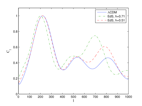
Figure 1: CMB angular power spectra for the $\Lambda$CDM model and two Einstein-de Sitter models, normalized to the height of the first Doppler peak

In our case, we must use expression (22) for the angular diameter distance to the last scattering surface when we calculate the shift parameter in Eq. (32). On the other hand, we can still use the expression for the sound horizon as defined in the homogeneous case in Eq. (25), since our model is assumed to be homogeneous close to the last scattering surface.

IV Results

When going from a homogeneous to an inhomogeneous universe model, the parameters describing the model ($\omega_{m}$ and $\omega_{k}$) become functions of $r$. This means that we introduce, in principle, an infinite number of new degrees of freedom. However, for the purpose of studying the possibility of explaining the current observations without introducing dark energy into the model, we have restricted ourselves to a very simple “toy model”: An underdense region close to us, surrounded by a flat, matter dominated universe. This means that we must choose $\alpha_{0}=1$ and $\beta_{0}=0$. Furthermore, we put $\Delta\alpha=-\Delta\beta$. This leaves four parameters, $\Delta\alpha$, $r_{0}$, $\Delta r$ and the physical Hubble parameter at the origin, $H_{\parallel}(0,t_{0})=100h\,\mathrm{\frac{km}{s\cdot Mpc}}$, to be fitted to the observations.

Let us first focus on the two main observations: The supernova Hubble diagram and CMB angular power spectrum. A good fit to the supernova data requires the Hubble parameter inside the underdensity, $h_{\text{in}}$ to be around $h_{\text{in}}\simeq 0.65$. On the other hand, a good fit to the CMB spectrum for a flat matter dominated model requires the Hubble parameter outside the underdensity to be $h_{\text{out}}\simeq 0.5$. This more or less determines the two parameters $\Delta\alpha$ and $h$.

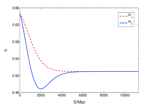
Figure 2: The spatial variation of the Hubble-parameters at $t=t_{0}$

Next, the shape of the transition between the underdense and the homogeneous region is specified by $r_{0}$ and $\Delta r$. These values dictate the redshift-magnitude relationship, and must be chosen to fit the supernova Hubble diagram. There are lots of choices for the parameters that give a very good fit to both the supernovae and the position of the first acoustic peak in the temperature power spectrum. However, we want the underdensity in our model to be such that the matter density is compatible with the current model independent observations of $\Omega_{m0}$. An excellent candidate for such observations is the mass-to-light ratio measurements made by the 2dF team Cross et al. (2001). These yield $\Omega_{m0}=0.24\pm 0.05$ from observations of galaxies with redshifts $z<0.12$. We will therefore choose the free parameters such that the mass density parameter at the origin is within this range in addition to giving a good fit to the supernova measurements and the CMB peak. The model which we adopt as our “standard model” gives a matter density at the center of the underdensity of $\Omega_{m0}=0.20$. A plot of the spatial variation today of the Hubble parameters of our standard model is given in figure 2. Furthermore, a plot of the distance modulus of this model together with the supernova observations can found in figure 3 .

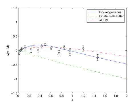
Figure 3: Distance modulus vs. redshift for our standard model together with supernova observations

Note that the $\chi^{2}$-value for our model is $\chi^{2}=176.5$, when compared to the “gold” dataset of Riess et al. Riess et al. (2004). This is slightly better than that of the concordance $\Lambda$CDM model Riess et al. (2004), $\chi^{2}_{\Lambda CDM}=178$.

The spatial shapes of the underdensity at the initial time and today are plotted in figure 4 as functions of the physical distance today. This illustrates the time evolution of the underdensity. As we can see, the shape stays almost constant. This is due to the Hubble parameters $H_{\parallel}$ and $H_{\perp}$ being roughly constant in space.

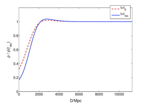
Figure 4: The evolution of the underdensity in our standard model

Although the matter distribution is clearly inhomogeneous close to the observer, we wish to point out that this does not necessarily contradict the data from the galaxy surveys. One often hears the claim that these surveys show the local distribution of matter to be homogeneous. However, it is probably more correct to say that they are shown to be compatible with a homogeneous universe rather than actually proving it. The key point here is that in order to determine for example the number counts of galaxy clusters, one needs to make an assumption about galaxy evolution and how likely it is to observe a galaxy with a certain luminosity at a certain redshift. As pointed out in e.g. Mustapha et al. (1997), one usually assumes a homogeneous universe in order to deduce the effects of source evolution. Therefore, using this deduced evolution to claim observed homogeneity in the number counts amounts only to circular argumentation. Furthermore, it is explicitly shown in Mustapha et al. (1997) that given any LTB model it is always possible to find a source evolution that agrees with the observed number counts.

The inhomogeneity at the center gives only a minor change of the angular diameter distance to the last scattering surface. In fact, our model has $d_{A}=10.4\,\mathrm{Mpc}$, which is the same value as we find for the Einstein-de Sitter model with $h=0.51$. (Note that these values are physical, not comoving distances). Our model, with Hubble parameter $h\simeq 0.51$ in the homogeneous region, thus yields a CMB angular power spectrum very similar to the one plotted in figure 1, at least for large $l$ values. Using the formula (32), we find $\mathcal{S}=1.006$, i.e. an almost perfect match for the position of the first Doppler peak. For smaller $l$ values, the CMB pattern will be affected by our position relative to the center of the underdensity. This has been studied in the previously mentioned void model of Tomita Tomita (2000), who concluded that relatively large displacements from the center of the underdensity were fully consistent with the observed CMB dipole and quadrupole. Furthermore, J. Moffat Moffat (2005) argues that such a displacement could even explain the detected alignment of the CMB quadru- and octopole Schwarz et al. (2004).

A rough estimate of the apparent peculiar velocity for an off-center observer is Tomita (2000)

$$v_{p}\simeq\left(h_{\parallel,\text{in}}-h_{\parallel,\text{out}}\right)l_{0}\cdot 100\,\mathrm{km/s}$$ (33)

where $l_{0}$ is the distance from the observer to the center, measured in Mpc. If we for instance require that $v_{p}$ must be less than the estimated peculiar velocity of the local group Kogut et al. (1993), which is of the order of 600 km/s, this means that the observer must be within $40\,\mathrm{Mpc}$ from the center of the inhomogeneity. Even stronger constraints might be obtained by considering the peculiar velocities of nearby clusters, see e.g. Hudson et al. (2004).

Recently, Eisenstein et al. announced the detection of baryon oscillations in the SDSS galaxy power spectrum Eisenstein et al. (2005). This represents additional, independent data that can be used to constrain our model even further. The physical length scale associated with these oscillations is set by the sound horizon at recombination. Measuring how large this length scale appears at some redshift in the galaxy power spectrum allows us to constrain the time evolution of the universe from recombination to the time corresponding to this redshift Hu and Sugiyama (1996); Eisenstein and Hu (1998); Hu and Haiman (2003); Blake and Glazebrook (2003); Linder (2003, 2005).

A length scale quoted by Eisenstein et al. is the ratio of the effective distance to the chosen redshift in the galaxy survey to the angular diameter distance to the last scattering surface,

$$R_{0.35}=\frac{d_{V}(z_{sdss})}{d_{A}(z_{*})}\,,$$ (34)

where $z_{sdss}=0.35$. The effective distance $d_{V}$ is defined in Eq. (2) in Ref. Eisenstein et al. (2005) as a mix of radial and angular distance, to take into account that these scale differently. The value they measure for this ratio is $R_{0.35}=79.0\pm 2.9$. Note that this value differs from that quoted in Eisenstein et al. (2005). The reason for this is that we’ve chosen to give the distances $d_{V}$ and $d_{A}$ in physical coordinates, while Eisenstein et al. quote them as comoving.

Calculating this ratio for our model we find the value $R_{0.35}^{inhom}=107.1$. Comparing this value with that quoted by Eisenstein et al., one might be tempted to claim that the model is ruled out. However, in order to say something conclusive using this constraint, we need to be sure that the “measured” value of $R_{0.35}$ is model independent. But when the authors derived this constraint they assumed a $\Lambda$CDM model. This makes it a little unclear how to use this constraint for non-$\Lambda$CDM models, or, indeed, whether it is even possible to use it for such models. Ideally, one would need to repeat the analysis of Eisenstein et al. assuming our inhomogeneous model as base model. We will therefore be careful not to rule out the model based on this parameter alone.

The main features of our standard model are summarized in table 1.

Description	Symbol	Value
Density contrast parameter	$\Delta\alpha$	0.90
Transition point	$r_{0}$	1.35 Gpc
Transition width	$\Delta r/r_{0}$	0.40
Fit to supernovae	$\chi^{2}_{SN}$	176.5
Position of first CMB peak	$\mathcal{S}$	1.006
Age of the universe	$t_{0}$	$12.8\,\mathrm{Gyr}$
Relative density inside underdensity	$\Omega_{m,in}$	0.20
Relative density outside underdensity	$\Omega_{m,out}$	1.00
Hubble parameter inside underdensity	$h_{in}$	0.65
Hubble parameter outside underdensity	$h_{out}$	0.51
Physical distance to last scattering surface	$D_{LSS}$	11.3 Gpc
Length scale of baryon oscillation from SDSS	$R_{0.35}$	107.1

Table 1: The parameters and features of our adopted standard inhomogeneous model

Note that the age of the universe is $12.8\,\mathrm{Gyr}$ in our model. This is significantly less than the value for the concordance $\Lambda$CDM model, $13.7\,\mathrm{Gyr}$, but it is still in agreement with observations of globular clusters Krauss and Chaboyer (2003), which put a lower limit of $11.2\,\mathrm{Gyr}$ on the age of the universe.

V Summary and conclusions

The main goal of this paper has been to present a simple model with the ability to explain the apparent accelerated expansion of the universe without the need to introduce dark energy. Inspired by the recent discussions about the possibility of explaining the apparent acceleration by inhomogeneities in the matter distribution, we have studied a model where the observer is assumed to be situated near the center of an underdense bubble in a flat, matter dominated universe. If this model is realistic, we live in a perturbed Einstein-de Sitter universe within 130 million light years from the center of an underdensity that extends about 5 billion light years outwards. Under the assumption of spherical symmetry this universe is described by the Lemaître-Tolman-Bondi space-time.

The two main observations we sought to explain were the luminosity distance-redshift relation inferred from SNIa observations and the CMB temperature power spectrum. These two sets of observations are made at opposite ends of the redshift spectrum, respectively low redshifts for the supernovae and high redshifts for the CMB. The fact that our model is inhomogeneous allows us therefore to choose the geometry and matter distribution such that the physical conditions are favourable for explaining the SNIa at low redshift while they at the same time are favourable for explaining the CMB at high redshifts. We find that a very good fit to the supernova data is obtained if we allow the transverse Hubble parameter to decrease with the distance from the observer. On the other hand, we get a good fit to the location of the first peak of the CMB power spectrum if we assume the universe to be flat with a value of $0.51$ for the Hubble parameter outside the inhomogeneity. Interpolating between these two limiting behaviours we get a good fit to both the supernova data and the location of the first peak.

Our model yields a better fit to the Riess data set of supernovae than the concordance $\Lambda$CDM model. However, for the CMB fit we tested only for the location of the first peak. Although the model yields a good fit to this, it does not necessarily mean that it matches the whole CMB spectrum. Indeed, since the physics responsible for the acoustic peaks is determined by the pre-recombination era, we would expect the peaks to look more or less the same as for a flat, homogeneous model with $h=0.51$. This suggests that our model might fail to explain the third peak. Furthermore, the model does not appear to be able to explain the observed length scale of the baryon oscillations in the SDSS matter power spectrum either, although one may question whether the data quoted by the SDSS team can be used directly to test our model.

The most powerful way to rule out inhomogeneous universe models would be to do a full analysis of the evolution of perturbations in these models. In that way, one could confront the model with both the full CMB angular power spectrum and the matter power spectrum. Only after such an analysis is carried out can one say whether our model is ruled out or if it is a viable alternative to dark energy.