What galaxies know about their nearest cluster

Abstract

We investigate the extent to which galaxies’ star-formation histories and morphologies are determined by their clustocentric distance and their nearest cluster’s richness. We define clustocentric distance as the transverse projected distance between a galaxy and its nearest cluster center within $\pm 1000~{}\mathrm{km\,s^{-1}}$. We consider a cluster to be a bound group of at least $N_{\mathrm{gal}}$ galaxies brighter than $M_{r}=-19$ mag; we employ different richness criteria of $N_{\mathrm{gal}}=5$, 10, and 20. We look at three tracers of star-formation history (${}^{0.1}i$ band absolute magnitude $M_{{}^{0.1}i}$, ${}^{0.1}[g-r]$ color, and $\mathrm{H}\alpha$ emission line equivalent width) and two indicators of galaxy morphology (surface brightness and radial concentration) for 52,569 galaxies in the redshift range of $0.015<z<0.068$. We find that our morphology indicators (surface brightness and concentration) relate to the clustocentric distance only indirectly through their relationships with stellar population and star formation rate. Galaxies that are near the cluster center tend to be more luminous, redder and have lower $\mathrm{H}\alpha$ EW (i.e., lower star-formation rates) than those that lie near or outside the virial radius of the cluster. The detailed relationships between these galaxy properties and clustocentric distance depend on cluster richness. For richer clusters, we find that (i) the transition in color and $\mathrm{H}\alpha$ EW from cluster center to field values is more abrupt and occurs closer to the cluster virial radius, and (ii) the color and $\mathrm{H}\alpha$ EW distributions are overall narrower than in less rich clusters. We also find that the radial gradient seen in the luminosity distribution is strongest around the smaller clusters and decreases as the cluster richness (and mass) increases. We find there is a “characteristic distance” at around one virial radius (the infall region) where the change with radius of galaxy property distributions is most dramatic, but we find no evidence for infall-triggered star bursts. These results suggest that galaxies “know” the distance to, and the size of, their nearest cluster and they express this information in their star-formation histories.

1 Introduction

The statistical properties of galaxies are closely related to the densities of their surrounding environments. Since regions of the Universe with different densities evolve at different rates, we expect these environment dependencies to contain crucial information about galaxy formation and evolution.

Much of previous environment-related work focused on the relationship between morphology and environment (Hubble 1936; Oemler 1974; Dressler 1980; Postman & Geller 1984; or the more recent work of Hermit et al. 1996; Guzzo et al. 1997; Giuricin et al. 2001; Trujillo et al. 2002). All these works find that bulge-dominated galaxies are more strongly clustered than disk-dominated galaxies. Spectroscopic and photometric properties of galaxies are strongly correlated with morphology so it is not surprising to find that the spectroscopic and photometric properties of galaxies are also functions of clustering (Kennicutt, 1983; Hashimoto et al., 1998; Balogh et al., 2001; Martínez et al., 2002; Lewis et al., 2002; Norberg et al., 2002; Hogg et al., 2003, 2004; Kauffmann et al., 2004; Zehavi et al., 2005). While trying to understand why these properties relate with environment, it is important to ask which properties are correlated with environment independently of the others. Previous work has found that, out of color, luminosity, surface brightness, and Sérsic index (concentration), the color and luminosity of a galaxy appear to be the only properties that are directly related to the local overdensity (Blanton et al., 2005a). Surface brightness and concentration appear to be related to the environment only through their relationships with color and luminosity.

The clustocentric distance—the distance to the nearest rich cluster center—is a fundamental and precisely measurable environment indicator; indeed it can be measured at much higher signal-to-noise than estimates of overdensity on fixed scales. Previous observational results that use the clustocentric distance as an environment indicator have found that the star-formation rates of galaxies are correlated with the clustocentric distance in the following ways: (i) the star-formation rates of galaxies near the centers of clusters are low and they rise with increasing clustocentric distance. (ii) the correlation is steeper for galaxies with higher star-formation rates, and (iii) there is a ‘characteristic break’ at a distance of 3-4 cluster virial radii at which the change in the correlation is greatest (Lewis et al., 2002; Gomez et al., 2003). It has been suggested that gas-stripping plays a significant role in this rapid truncation of star-formation, as well as the morphological transformation that is observed in the cluster population (Vogt et al., 2004), although most statistical studies find that this process cannot be extremely rapid (Kodama & Bower, 2001; Balogh et al., 2000). Models generally find that the star-formation rates of cluster galaxies depend primarily on the time elapsed since their accretion onto the massive system, but that the cessation of star formation may take place gradually over a few billion years (Balogh et al., 2000).

In this short paper, we build upon previous studies in several ways. We use the Berlind et al. (2006) cluster catalog that was created with a different algorithm than previous studies. In particular, the algorithm did not use galaxy colors in the group and cluster identification, so our galaxy colors are unbiased even in the cluster cores. Moreover, the cluster catalog was designed to recover clusters of galaxies that occupy the same underlying dark matter halo. Consequently, the abundance of these clusters is unbiased relative to the abundance of halos and can thus be used to obtain robust estimates of the cluster masses. The method we use to estimate cluster masses differs significantly from the methods used in previous studies. This difference leads to a different conclusion regarding the activity observed in the theoretically active infall regions around clusters. Finally, we examine the relationship between the morphology–environment relation and the color–environment relation.

We use the Sloan Digital Sky Survey (SDSS) data to measure the clustocentric distances of $\sim 52,000$ galaxies relative to $\sim 950$ clusters within the redshift range $0.015<z<0.068$. We use high quality photometric and spectroscopic data to examine the dependence of ${}^{0.1}[g-r]$ color, absolute magnitude $M_{{}^{0.1}i}$, $\mathrm{H}\alpha$ equivalent width (EW), concentration (Sérsic index), and surface brightness $\mu_{{}^{0.1}i}$ on both clustocentric distance and cluster richness. The large solid angular coverage of the SDSS permits the study of galaxies from cluster centers through the “infall regions” (Poggianti et al., 1999; Balogh et al., 2000; Kodama & Bower, 2001) and out to huge clustocentric distances.

In what follows, a cosmological world model with $(\Omega_{\mathrm{M}},\Omega_{\mathrm{\Lambda}})=(0.3,0.7)$ is adopted, and the Hubble constant is parameterized $H_{0}\equiv 100\,h~{}\mathrm{km\,s^{-1}\,Mpc^{-1}}$, for the purposes of calculating distances and volumes with $h=1$ except where otherwise noted (e.g., Hogg, 1999).

2 Data

The SDSS is taking $ugriz$ CCD imaging of $\sim 10^{4}~{}\mathrm{deg^{2}}$ of the Northern Galactic sky, and, from that imaging, selecting $\sim 10^{6}$ targets for spectroscopy, most of them galaxies with $r<17.77~{}\mathrm{mag}$ (e.g., Gunn et al., 1998; York et al., 2000; Stoughton et al., 2002). All the data processing, including astrometry (Pier et al., 2003), source identification, deblending and photometry (Lupton et al., 2001), calibration (Fukugita et al., 1996; Smith et al., 2002), spectroscopic target selection (Eisenstein et al., 2001; Strauss et al., 2002; Richards et al., 2002), spectroscopic fiber placement (Blanton et al., 2003a), spectral data reduction and analysis (Schlegel & Burles, in preparation, Schlegel in preparation) are performed with automated SDSS software.

Galaxy colors are computed in fixed bandpasses, using Galactic extinction corrections (Schlegel et al., 1998) and $K$ corrections (computed with kcorrect v3_2; Blanton et al., 2003). They are $K$ corrected, not to the redshift $z=0$ observed bandpasses, but to bluer bandpasses ${}^{0.1}g$, ${}^{0.1}r$ and ${}^{0.1}i$ “made” by shifting the SDSS $g$, $r$, and $i$ bandpasses to shorter wavelengths by a factor of 1.1 (c.f., Blanton et al., 2003, 2003b). This means that galaxies at redshift $z=0.1$ all have the same $K$ corrections: $K(0.1)=-2.5\log(1.1)$.

For the purposes of computing large-scale structure statistics, we have assembled a complete subsample of SDSS galaxies known as the NYU LSS sample14. This subsample is described elsewhere (Blanton et al., 2005b); it is selected to have a well-defined window function and magnitude limit. In addition, the sample of galaxies used here was selected to have apparent magnitude in the range $14.5<r<17.77~{}\mathrm{mag}$, redshift in the range $0.015<z<0.068$, and absolute magnitude $M_{{}^{0.1}i}>-24~{}\mathrm{mag}$. These cuts left 52,569 galaxies.

A seeing-convolved Sérsic model is fit to the azimuthally averaged radial profile of every galaxy in the observed-frame $i$ band, as described elsewhere (Blanton et al., 2003b; Strateva et al., 2001). The Sérsic model has surface brightness $I$ related to angular radius $r$ by $I\propto\exp[-(r/r_{0})^{(1/n)}]$, so the parameter $n$ (Sérsic index) is a measure of radial concentration (seeing-corrected). At $n=1$ the profile is exponential, and at $n=4$ the profile is de Vaucouleurs. In the fits shown here, values in the range $0.5<n<5.5$ were allowed.

To every best-fit Sérsic profile, the Petrosian (1976) photometry technique is applied, with the same parameters as used in the SDSS survey. This supplies seeing-corrected Petrosian magnitudes and radii. A $K$-corrected surface-brightness $\mu_{{}^{0.1}i}$ in the ${}^{0.1}i$ band is computed by dividing half the $K$-corrected Petrosian light by the area of the Petrosian half-light circle.

The $\mathrm{H}\alpha$ line flux is measured in a 20 Å width interval centered on the line. Before the flux is computed, a best-fit model A+K spectrum (Quintero et al., 2004) is scaled to have the same flux continuum as the data in the vicinity of the emission line and subtracted to leave a continuum-subtracted line spectrum. This method fairly accurately models the $\mathrm{H}\alpha$ absorption trough in the continuum, although in detail it leaves small negative residuals. The flux is converted to a rest-frame EW with a continuum found by taking the inverse-variance-weighted average of two sections of the spectrum about 150 Å in size and on either side of the emission line. Further details are presented elsewhere (Quintero et al., 2004).

A caveat to this analysis is that the 3 arcsec diameter spectroscopic fibers of the SDSS spectrographs do not obtain all of each galaxy’s light because at redshifts of $0.015<z<0.068$ they represent apertures of between $0.6$ and $2.7~{}h^{-1}\,\mathrm{kpc}$ diameter. The integrity of our $\mathrm{H}\alpha$ EW measurement is a function of galaxy size, inclination, and morphology. We have looked at variations in our $\mathrm{H}\alpha$ EW results as a function of redshift and found that the quantitative results differ but our qualitative results remain the same.

For each galaxy, a selection volume $V_{\mathrm{max}}$ is computed, representing the total volume of the Universe (in $h^{-3}~{}\mathrm{Mpc^{3}}$) in which the galaxy could have resided and still made it into the sample. The calculation of these volumes is described elsewhere (Blanton et al., 2003c, b). For each galaxy, the quantity $1/V_{\mathrm{max}}$ is that galaxy’s contribution to the cosmic number density.

We use the group and cluster catalog described in Berlind et al. (2006). The catalog is obtained from a volume-limited sample of galaxies that is complete down to an ${}^{0.1}r$ band absolute magnitude of $M_{r}<-19$ mag and goes out to a redshift of 0.068. Groups are identified using a friends-of-friends algorithm (see e.g., Geller & Huchra 1983; Davis et al 1985) with perpendicular and line-of-sight linking lengths equal to 0.14 and 0.75 times the mean inter-galaxy separation, respectively. These parameters were chosen with the help of mock galaxy catalogs to produce galaxy groups that most closely resemble galaxy systems that occupy the same dark matter halos; i.e., that are bound. The resulting catalog contains 944 systems with a richness $N_{\mathrm{gal}}\geq 5$ member galaxies. For consistency, we call these objects “clusters”. Note that, unlike some other catalogs, galaxy colors are not used in cluster identification.

Berlind et al. (2006) calculate rough mass estimates for the clusters using the cluster luminosity function (where luminosity is defined as the total luminosity in $M_{r}<-19$ mag galaxies in the cluster) and assuming a monotonic relation between a cluster’s luminosity and the mass of its underlying dark matter halo. By matching the measured space density of clusters to the theoretical space density of dark matter halos (given the concordance cosmological model and a standard halo mass function), they assign a virial halo mass to each cluster luminosity. The masses derived in this way ignore the scatter in mass at fixed cluster luminosity and are only meant to be rough estimates. The resulting masses for the clusters used here range from $\sim 10^{12}$ to $\sim 10^{15}$ solar masses. Each cluster has an associated “virial radius” of

$$R_{\mathrm{vir}}=\left(\frac{3}{4\,\pi}\frac{M}{200\,\rho_{o}}\right)^{\frac{1}{3}}\quad,$$ (1)

where $M$ is the estimated mass of the cluster and $\rho_{o}$ is the current mean density of the Universe. Note that this method for determination of the virial radii is very different from that employed by other investigators. Some have used a quasi-empirical formula based on velocity dispersion (Gomez et al., 2003; Christlein & Zabludoff, 2005), others have assumed that cluster mass is directly proportional to richness (Lewis et al., 2002); in general these methods differ substantially, and thus produce cluster catalogs with very different mass functions.

We use the cluster centers given by Berlind et al. (2006), which are computed as the mean of the member galaxy positions. We then calculate the transverse projected clustocentric distance $D_{\mathrm{cl}}$ from each galaxy to its nearest cluster center on the sky within $\pm 1000~{}\mathrm{km\,s^{-1}}$ in radial velocity. We split the cluster catalog into three richness bins. The small, medium, and large richness bins contain clusters with 5 to 9, 10 to 19, and 20 or greater galaxies with $M_{r}<-19$ mag, respectively. We associate galaxies to their nearest large cluster, even if they are also nearby a smaller cluster; for example, a galaxy whose nearest cluster has a richness of $5\leq N_{\mathrm{gal}}\leq 9$ falls into the “small” richness bin. If this galaxy also has a nearby cluster of richness $10\leq N_{\mathrm{gal}}\leq 19$ it would also fall into the “medium” richness bin, but with a $D_{\mathrm{cl}}$ which corresponds to this different cluster.

3 Results

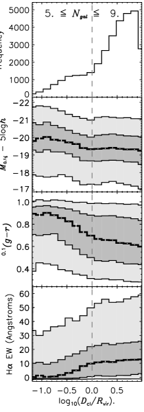
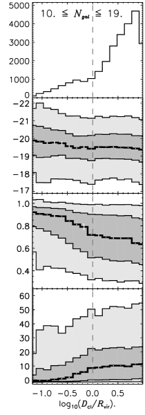
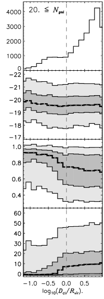
Figure 1: The dependence of the 5, 25, 50 (bold), 75, and 95 percent $V_{\mathrm{max}}$-weighted quantiles of several galaxy properties on $D_{\mathrm{cl}}$, shown for 3 different cluster-richness bins. The “weighted quantile” is defined as follows: The 5th percentile weighted quantile has 5 percent of the total weight below it and 95 percent above it. The top panel of each column shows the $D_{\mathrm{cl}}$ distribution of galaxies in the specified richness bin. The other panels show the dependencies of the quantiles of absolute magnitude $M_{{}^{0.1}i}$ , ${}^{0.1}[g-r]$ color, and $\mathrm{H}\alpha$EW on $D_{\mathrm{cl}}$. The figures are shaded to guide the eye. The errors in the 50 percent quantiles, calculated using the jackknife method (10 jackknife trials, separated by constant declination lines, in each of which 1/10 of the survey footprint is dropped) are overplotted in white.

We first examine the relation between three tracers of star-formation history and clustocentric distance. Figure 1 shows the relationship between clustocentric distance and quantiles of three $1/V_{\mathrm{max}}$-weighted galaxy properties: absolute magnitude $M_{{}^{0.1}i}$, ${}^{0.1}[g-r]$ color and $\mathrm{H}\alpha$ EW for the three different richness bins. All three properties show a dependence on clustocentric distance. In agreement with previous work, we find that galaxies near the centers of clusters are more luminous, redder and lower in $\mathrm{H}\alpha$ EW than galaxies in the field.

For all three galaxy properties there is a change of slope or “break” in the quantile gradients at around one virial radius, regardless of richness. The break seen in $\mathrm{H}\alpha$ EW is similar to that found by Gomez et al. (2003), except that they found this break at a distance of 3-4 virial radii, whereas this figure shows it occurs at $D_{\mathrm{cl}}\,\sim\,R_{\mathrm{vir}}$. This discrepancy can be attributed to the different methods of determining the virial radius. Our estimates of $R_{\mathrm{vir}}$ are based on cluster abundances (Berlind et al., 2006), whereas Gomez et al. (2003) use the Girardi et al. (1998) approximation relating $R_{\mathrm{vir}}$ to velocity dispersion. We discuss this more in § 4.

Although all these trends in galaxy properties display a break near $R_{\mathrm{vir}}$, Figure 1 shows that the strength of the trends depends on cluster richness, $N_{\mathrm{gal}}$. The different $M_{{}^{0.1}i}$ panels demonstrate that the $M_{{}^{0.1}i}$ vs. $D_{\mathrm{cl}}$ gradient is larger for the smaller clusters. In other words, as one approaches the center of a cluster, the increase in typical luminosity is greater for smaller clusters. The ${}^{0.1}[g-r]$ vs. $D_{\mathrm{cl}}$ gradient depends on cluster richness in the following two ways: (i) the transition in typical galaxy color from the cluster center (i.e., redder) to the field value (i.e., bluer) is more abrupt and occurs closer to $R_{\mathrm{vir}}$ for larger clusters and (ii) the color distribution is overall narrower within larger clusters. Similar to color, the $\mathrm{H}\alpha$ EW vs. $D_{\mathrm{cl}}$ gradient depends on cluster richness in the following two ways: (i) the transition in typical $\mathrm{H}\alpha$ EW from the cluster center (i.e., lower) to the field value (i.e., higher) is more abrupt and occurs closer to $R_{\mathrm{vir}}$ for larger clusters and (ii) the $\mathrm{H}\alpha$ EW distribution is overall narrower within larger clusters.

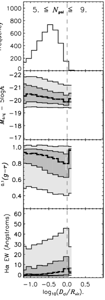
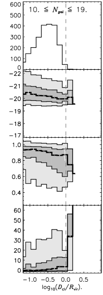
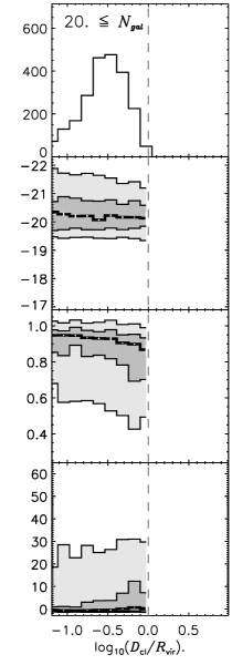
Figure 2: Similar to Figure 1, except for galaxies that Berlind et al. (2006) have determined to be members of their closest clusters. All trends are affected (relative to Figure 1) by the magnitude cut of $M_{r}<-19$ mag in the cluster definition; in particular, the $M_{{}^{0.1}i}$ panels are strongly affected.

The plots in Figure 1 include all galaxies within $\pm 1000~{}\mathrm{km\,s^{-1}}$ of each cluster center, so galaxies in the foreground and background of the cluster contribute to this Figure. To investigate whether these projection effects (such as the presence of “infall interlopers” discussed by Rines et al. 2005) significantly influence the observed trends, we made the same plot in Figure 2, but showing only the cluster members (i.e., the galaxies that are members of their closest cluster). Figure 2 shows that there are still dependences on clustocentric distance. The trends are not as strong as in Figure 1 because this subset of the data has a smaller absolute magnitude range. There is a cut of $M_{{}^{0.1}r}<-19$ mag on this subset due to the cluster definition. When we make the same $M_{{}^{0.1}r}$ cut on the sample used in Figure 1, the trends look the same as they do in this Figure. The result of this comparison suggests two things: first, effects due to projection (i.e., due to galaxies with small $D_{\mathrm{cl}}$ but not spatially close to the cluster center) are small and don’t affect our results and, second, the fainter galaxies contribute more to these trends than the brighter ones.

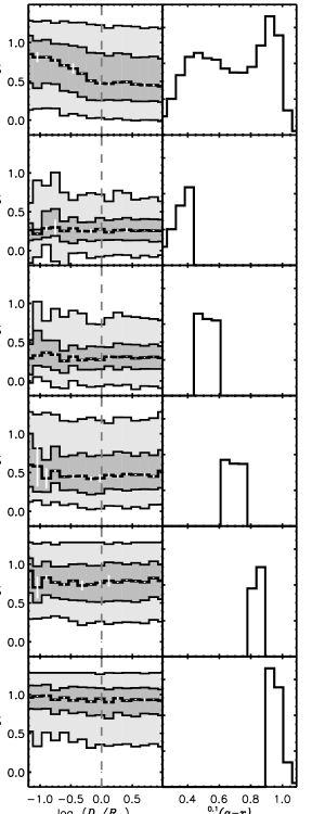
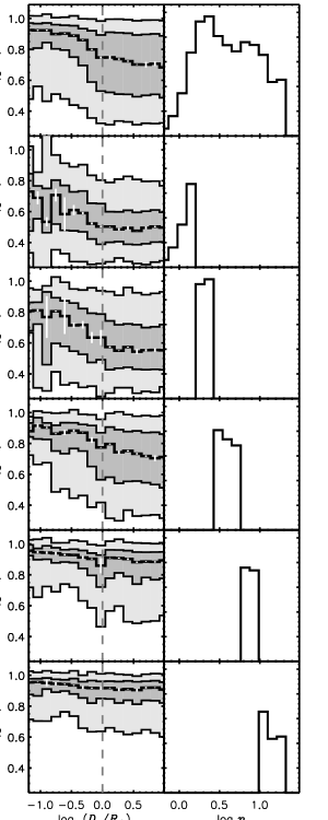
Figure 3: The dependence of radial concentration $n$ (left figure) and ${}^{0.1}[g-r]$ color (right figure) on clustocentric distance $D_{\mathrm{cl}}$ for the smallest richness bin sample: $5\leq N_{\mathrm{gal}}\leq 9$. For the figure on the left, the top-left panel shows how the quantiles of Sérsic index $n$ depend on $D_{\mathrm{cl}}$ for the whole sample. The top-right panel of this figure shows the ${}^{0.1}[g-r]$ color distribution of the sample. The subsequent rows show the same for narrow color subsamples described by the color distributions shown in the right column. All the panels in the left column have the same layout as Figure 1. The figure on the right is very similar but with the $n$ and ${}^{0.1}[g-r]$ properties interchanged. Notice the dependence of concentration on clustocentric distance almost vanishes in each color subsample while the dependence of color on clustocentric distance remains in each concentration subsample. These phenomena were also observed for the other two richness bin samples: $10\leq N_{\mathrm{gal}}\leq 19$ and $20\leq N_{\mathrm{gal}}$.

Figures 1 and 2 show how our tracers of star-formation history depend on clustocentric distance and cluster richness. Blanton et al. (2005a) found that morphology tracers, such as concentration and surface brightness, only depend on local overdensity through their correlation with star-formation history. This has not been demonstrated for clustocentric radius, which is a much higher signal-to-noise environment estimator than local overdensity. We investigate this in Figure 3.

The left half of Figure 3 shows the the relation between the Sérsic index $n$ (concentration) and clustocentric distance for different color bubsamples (left panels), as well as the 1/Vmax-weighted distribution of ${}^{0.1}[g-r]$ color for each subsample (right panels). The dependence of concentration on clustocentric distance for the whole sample is shown in the top row, and for narrow color subsamples in the following rows. Similar to previous results (Blanton et al., 2005a), we find that this dependence of concentration on clustocentric distance almost completely vanishes within narrow color subsamples. The right half of Figure 3 is similar, but with the concentration $n$ and ${}^{0.1}[g-r]$ color properties interchanged. The dependence of color on clustocentric distance remains even within the narrow concentration subsamples. We therefore conclude that the dependence of concentration $n$ on clustocentric distance is simply due to the dependence of concentration on color combined with the dependence of color on clustocentric distance. There is very little independent dependence of concentration on clustocentric distance. Surface brightness $\mu_{{}^{0.1}i}$ shows the same behavior as concentration.

It is worth mentioning that galaxies that contain active galactic nuclei (and therefore have $\mathrm{H}\alpha$ EW not entirely due to star formation) have a negligible effect on these results. These results and figures do not change substantially when we remove the AGN galaxies, as defined elsewhere (Kauffmann et al., 2003). We also note that “edge effects” from the survey boundaries do not alter our results; there is little change to the figures and results when we remove galaxies and clusters that lie near the survey edges. Finally, our results are not sensitive to the choice of definition for cluster centers. We have verified that the results do not change significantly if we assume that a cluster’s center is at the position of its most luminous galaxy, rather than the centroid of all its galaxy positions.

4 Discussion

Using a complete sample of 52,569 galaxies in the redshift range of $0.015<z<0.068$ we examine how ${}^{0.1}i$ band absolute magnitude $M_{{}^{0.1}i}$, ${}^{0.1}[g-r]$ color, $\mathrm{H}\alpha$ EW, surface brightness, and concentration are related to both the transverse projected clustocentric distance, $D_{\mathrm{cl}}$, and the richness, $N_{\mathrm{gal}}$, of its nearest cluster. Similar to previous results (Blanton et al., 2005a; Christlein & Zabludoff, 2005), we find that our morphology tracers (concentration and surface brightness) appear to be related to environment ($D_{\mathrm{cl}}$  in this case) only indirectly through their relationships with the star-formation history tracers. This suggests that the well known morphology–environment relation is a residual of the star-formation-history–environment relation. We note that, although our simple morphology indicators do not show direct dependence on clustocentric distance, this result does not disagree with that the original morphology–density studies (Hubble, 1936; Oemler, 1974; Dressler, 1980; Postman & Geller, 1984) because these studies did not attempt to separate morphological and star-formation dependences. Our results also do not disagree with previous work (Vogt et al., 2004) which suggests that gas stripping plays a significant role in the morphological transformation and rapid truncation of star formation by showing asymmetries in HI and $\mathrm{H}\alpha$ flux on the leading edge of infalling spiral galaxies. There is no disagreement because our very blunt morphology indicators are insensitive to these asymmetries.

We have shown that galaxies know about the distance to, and richness of, their nearest cluster and they express that knowledge most clearly through their star-formation histories. Some morphological evidence suggests that they also know the direction as well (Vogt et al., 2004).

Where our results overlap those of previous investigators (Lewis et al., 2002; Gomez et al., 2003; Blanton et al., 2005a), we mostly find good agreement. In particular, we find that galaxy properties depend on clustocentric distance much the same way as they do on other environmental indicators (Blanton et al., 2005a). Our result improves on this previous one because the clustocentric distance is measured at much higher signal-to-noise and probes environments on scales much smaller than local overdensity measurements. Where our results disagree with previous work, it can mainly be attributed to the different methods of computing cluster virial radii. While it may seem that this is a minor discrepancy, these disagreements become important at the interpretation level. In particular, the claim that clusters affect galaxies well beyond the cluster virial radii (Lewis et al., 2002; Gomez et al., 2003) depends strongly on the calculation of virial radius. Our virial radii are estimated from cluster abundances (and an assumed “concordance” cosmological model), whereas in previous work they are estimated from cluster velocity dispersions. In order to check the difference between these two methods, we computed a second set of virial radii for our clusters using the Berlind et al. (2006) velocity dispersions and the Girardi et al. (1998) approximation that relates virial radius to velocity dispersion. We find that the virial radii based on velocity dispersions are systematically lower than those based on abundances by a factor of two to three. This is sufficient to explain the difference in interpretation between Gomez et al. (2003) and this work. We choose to measure our virial radii using cluster abundances because the Berlind et al. (2006) cluster catalog was tuned to produce unbiased abundances and we, therefore, believe them to be less subject to systematic errors than velocity dispersion estimates. However, this point deserves to be studied in more detail.

After analyzing these results, we are in a position to address the theoretically active “infall region” (Poggianti et al., 1999; Balogh et al., 2000; Kodama & Bower, 2001) around virialized systems. All three trends (color, $\mathrm{H}\alpha$, and absolute magnitude) as a function of $D_{\mathrm{cl}}$ have a “characteristic break” at about the same virial-radius-normalized distance from the cluster center but we find no clear evidence for an “increase” in star formation activity at the infall region.

Here we have investigated how galaxy colors, luminosities, and star-formation rates ($\mathrm{H}\alpha$ EW) relate to clustocentric distance and how these relations depend on cluster richness. We find that for larger clusters the transitions in the typical values of color and star-formation rate from cluster centers to the field are more abrupt and occur closer to the viral radius than those for smaller clusters. We also find the increase in typical luminosity when looking from the field to cluster centers is greater around smaller clusters. A question that naturally arises is: What physical physical processes are involved in creating these richness-dependent variations? It could be that (i) the possible transformation mechanisms are stronger in larger clusters (e.g., more frequent tidal interactions or a hotter intercluster medium), (ii) galaxies in larger clusters have been in this environment longer and therefore have had more time to evolve to their long-term properties, or (more likely) a combination of the two.

References

- Balogh et al. (2001) Balogh, M. L., Christlein, D., Zabludoff, A. I., & Zaritsky, D. 2001, ApJ, 557, 117
- Balogh et al. (2000) Balogh, M. L., Navarro, J. F., & Morris, S. L. 2000, ApJ, 540, 113
- Berlind et al. (2006) Berlind, A. A., Frieman, J. A., Weinberg, D. H., Blanton, M. R., Warren, M., Abazajian, K., Scranton, R., Hogg, D. W., & Scoccimarro, R. 2006, ApJ
- Blanton et al. (2003) Blanton, M. R., Brinkmann, J., Csabai, I., Doi, M., Eisenstein, D. J., Fukugita, M., Gunn, J. E., Hogg, D. W., & Schlegel, D. J. 2003, AJ, 125, 2348
- Blanton et al. (2005a) Blanton, M. R., Eisenstein, D., Hogg, D. W., Schlegel, D. J., & Brinkmann, J. 2005a, ApJ, 629, 143
- Blanton et al. (2003a) Blanton, M. R., Lin, H., Lupton, R. H., Maley, F. M., Young, N., Zehavi, I., & Loveday, J. 2003a, AJ, 125, 2276
- Blanton et al. (2003b) Blanton, M. R. et al. 2003b, ApJ, 594, 186
- Blanton et al. (2003c) Blanton, M. R. et al. 2003c, ApJ, 592, 819
- Blanton et al. (2005b) Blanton, M. R. et al. 2005b, AJ, 129, 2562
- Christlein & Zabludoff (2005) Christlein, D. & Zabludoff, A. I. 2005, ApJ, 621, 201
- Dressler (1980) Dressler, A. 1980, ApJ, 236, 351
- Eisenstein et al. (2001) Eisenstein, D. J. et al. 2001, AJ, 122, 2267
- Fukugita et al. (1996) Fukugita, M., Ichikawa, T., Gunn, J. E., Doi, M., Shimasaku, K., & Schneider, D. P. 1996, AJ, 111, 1748
- Girardi et al. (1998) Girardi, M., Giuricin, G., Mardirossian, F., Mezzetti, M., & Boschin, W. 1998, ApJ, 505, 74
- Giuricin et al. (2001) Giuricin, G., Samurović, S., Girardi, M., Mezzetti, M., & Marinoni, C. 2001, ApJ, 554, 857
- Gomez et al. (2003) Gomez, P. et al. 2003, ApJ, 584, 210
- Gunn et al. (1998) Gunn, J. E., Carr, M. A., Rockosi, C. M., Sekiguchi, M., et al. 1998, AJ, 116, 3040
- Guzzo et al. (1997) Guzzo, L., Strauss, M. A., Fisher, K. B., Giovanelli, R., & Haynes, M. P. 1997, ApJ, 489, 37
- Hashimoto et al. (1998) Hashimoto, Y., Oemler, A., Lin, H., & Tucker, D. L. 1998, ApJ, 499, 589
- Hermit et al. (1996) Hermit, S., Santiago, B. X., Lahav, O., Strauss, M. A., Davis, M., Dressler, A., & Huchra, J. P. 1996, MNRAS, 283, 709
- Hogg (1999) Hogg, D. W. 1999, astro-ph/9905116
- Hogg et al. (2003) Hogg, D. W. et al. 2003, ApJ, 585, L5
- Hogg et al. (2004) Hogg, D. W. et al. 2004, ApJ, 601, L29
- Hubble (1936) Hubble, E. P. 1936, The Realm of the Nebulae (New Haven: Yale University Press)
- Kauffmann et al. (2004) Kauffmann, G., White, S. D. M., Heckman, T. M., Ménard, B., Brinchmann, J., Charlot, S., Tremonti, C., & Brinkmann, J. 2004, MNRAS, 314
- Kauffmann et al. (2003) Kauffmann, G. et al. 2003, MNRAS, 346, 1055
- Kennicutt (1983) Kennicutt, R. C. 1983, AJ, 88, 483
- Kodama & Bower (2001) Kodama, T. & Bower, R. G. 2001, MNRAS, 321, 18
- Lewis et al. (2002) Lewis, I. et al. 2002, MNRAS, 334, 673
- Lupton et al. (2001) Lupton, R. H., Gunn, J. E., Ivezić, Z., Knapp, G. R., Kent, S., & Yasuda, N. 2001, in ASP Conf. Ser. 238: Astronomical Data Analysis Software and Systems X, Vol. 10, 269
- Martínez et al. (2002) Martínez, H. J., Zandivarez, A., Domínguez, M., Merchán, M. E., & Lambas, D. G. 2002, MNRAS, 333, L31
- Norberg et al. (2002) Norberg, P. et al. 2002, MNRAS, 332, 827
- Oemler (1974) Oemler, A. 1974, ApJ, 194, 1
- Petrosian (1976) Petrosian, V. 1976, ApJ, 209, L1
- Pier et al. (2003) Pier, J. R., Munn, J. A., Hindsley, R. B., Hennessy, G. S., Kent, S. M., Lupton, R. H., & Ivezić, Ž. 2003, AJ, 125, 1559
- Poggianti et al. (1999) Poggianti, B. M., Smail, I., Dressler, A., Couch, W. J., Barger, A. J., Butcher, H., Ellis, R. S., & Oemler, A. 1999, ApJ, 518, 576
- Postman & Geller (1984) Postman, M. & Geller, M. 1984, ApJ, 281, 95
- Quintero et al. (2004) Quintero, A. D. et al. 2004, ApJ, 602, 190
- Richards et al. (2002) Richards, G. et al. 2002, AJ, 123, 2945
- Rines et al. (2005) Rines, K., Geller, M. J., Kurtz, M. J., & Diaferio, A. 2005, AJ, 130, 1482
- Schlegel et al. (1998) Schlegel, D. J., Finkbeiner, D. P., & Davis, M. 1998, ApJ, 500, 525
- Smith et al. (2002) Smith, J. A., Tucker, D. L., et al. 2002, AJ, 123, 2121
- Stoughton et al. (2002) Stoughton, C. et al. 2002, AJ, 123, 485
- Strateva et al. (2001) Strateva, I. et al. 2001, AJ, 122, 1861
- Strauss et al. (2002) Strauss, M. A. et al. 2002, AJ, 124, 1810
- Trujillo et al. (2002) Trujillo, I., Aguerri, J. A. L., Gutiérrez, C. M., Caon, N., & Cepa, J. 2002, ApJ, 573, L9
- Vogt et al. (2004) Vogt, N. P., Haynes, M. P., Giovanelli, R., & Herter, T. 2004, AJ, 127, 3300
- York et al. (2000) York, D. et al. 2000, AJ, 120, 1579
- Zehavi et al. (2005) Zehavi, I. et al. 2005, ApJ, 630, 1