Revised Pulsar Spindown

Abstract

We address the issue of electromagnetic pulsar spindown by combining our experience from the two limiting idealized cases which have been studied in great extent in the past: that of an aligned rotator where ideal MHD conditions apply, and that of a misaligned rotator in vacuum. We construct a spindown formula that takes into account the misalignment of the magnetic and rotation axes, and the magnetospheric particle acceleration gaps. We show that near the death line aligned rotators spin down much slower than orthogonal ones. In order to test this approach, we use a simple Monte Carlo method to simulate the evolution of pulsars and find a good fit to the observed pulsar distribution in the $P-\dot{P}$ diagram without invoking magnetic field decay. Our model may also account for individual pulsars spinning down with braking index $n<3$, by allowing the corotating part of the magnetosphere to end inside the light cylinder. We discuss the role of magnetic reconnection in determining the pulsar braking index. We show, however, that $n\sim 3$ remains a good approximation for the pulsar population as a whole. Moreover, we predict that pulsars near the death line have braking index values $n>3$, and that the older pulsar population has preferentially smaller magnetic inclination angles. We discuss possible signatures of such alignment in the existing pulsar data.

1. Introduction

The current canonical pulsar paradigm is that of a magnetized rotating neutron star (see Mestel 1999 for a review). However, we feel that certain fundamental aspects of the paradigm still remain unclear.

One aspect of the paradigm which we hope to elucidate in the present work has to do with the way the neutron star spins down. A spinning down neutron star with mass $M_{*}$, radius $r_{*}$, and angular velocity $\Omega$ loses rotational kinetic energy at a rate

$$L=\frac{2}{5}M_{*}r_{*}^{2}\Omega\dot{\Omega}\ .$$ (1)

Here, $M_{*}\sim 1.4M_{\odot}$, $r_{*}\sim 10$ km, and $\dot{(...)}\equiv{\rm d}(...)/{\rm d}t$. Energy is lost through electromagnetic torques in the magnetosphere, although other physical processes have at times also been discussed (gravitational radiation, wind outflow, star-disk interaction, etc.).

To a first approximation, the stellar magnetic field may be considered as that of a rotating magnetic dipole. Even under such a simplification the general description of the stellar magnetosphere is a formidable three dimensional problem, since, in general, the magnetic and rotation axes do not coincide. Awaiting the development of the general theory, one can still derive important conclusions based on two idealized limiting cases which have been studied in great extent: the case of an aligned magnetic dipole rotating in an atmosphere with freely available electric charges (i.e. with ideal MHD conditions), and that of a misaligned magnetic dipole rotating in vacuum.

The neutron star is not surrounded by vacuum, and one needs to take into consideration the electric fields that develop and the electric currents that flow in the rotating charged magnetosphere (Goldreich & Julian 1969). The most recent numerical calculation of the simplest possible case, that of the magnetosphere of an aligned rotator in force-free approximation (Contopoulos 2005, hereafter C05), yielded the following rather general result for the electromagnetic energy loss

$$L_{\rm aligned}=\frac{4\Omega\Omega_{F}\psi_{\rm open}^{2}}{6c}\$$ (2)

(the quantities $\Omega_{F}$ and $\psi_{\rm open}$ are defined below). In that picture, the magnetosphere consists of a corotating region of closed fieldlines which extends up to a distance $r_{c}$ from the rotation axis, and an open fieldline region with enclosed magnetic flux

$$\psi_{\rm open}\equiv\frac{1}{2\pi}\int_{\rm open}{\bf B}\cdot{\rm d}{\bf S}=1.23\frac{B_{*}r_{*}^{3}}{2r_{c}},$$ (3)

where $B_{*}$ is the polar value of the magnetic field (Contopoulos, Kazanas & Fendt 1999, hereafter CKF; Gruzinov 2005; C05; Timokhin 2005; see also Appendix A). The above expression is valid when $r_{c}\gg r_{*}$. In the limit $r_{c}=r_{*}$, straightforward calculation yields $\psi_{\rm open}=B_{*}r_{*}^{2}/2$.

The neutron star spins down because of the establishment of a large scale poloidal electric current circuit flowing along open field lines, and returning along the edge of the open field line region (see CKF for a detailed description). The electric current that flows between the magnetic axis (characterized by $\psi=0$) and the edge of the open field line region (characterized by $\psi=\psi_{\rm open}$) generates the spindown torque which leads to eq. 2. The quantity $\Omega_{F}$ in eq. 2 is the angular frequency of rotation of the open field lines. It is set by the electric potential drop that develops accross open field lines, between the magnetic axis and the edge of the open field line region. This potential in the magnetosphere is in general smaller than the corresponding electric potential drop on the surface of the star. The difference between the two potential drops is just the particle acceleration gap potential which develops along open magnetic field lines in the vicinity of the polar cap. Consequently, the angular velocity of open field lines will in general be different (smaller) than $\Omega$. Models of particle acceleration and pair creation of rotation-powered pulsars yield values of the gap potential $V_{\rm gap}$ of the order of $10^{12}$ Volts (e.g. Hibschmann & Arons 2001). One can directly show (see Appendix B) that the above together with the simplifying assumption that $\Omega_{F}$ is uniform accross open field lines, yield

$$\Omega_{F}=\Omega-\Omega_{\rm death}\ ,$$ (4)

where,

$$\Omega_{\rm death}\equiv\frac{V_{\rm gap}}{\psi_{\rm open}}c\ .$$ (5)

This describes the so-called pulsar ‘death’, i.e. the stopping of pulsar emission. As the neutron star slows down and $\Omega$ drops below $\Omega_{\rm death}$, the gap potential cannot attain the value required for particle acceleration and consequent pulse generation, and the pulsar stops generating radio emission.

A misaligned dipole rotating in vacuum loses energy at a rate

$$L_{vacuum}=\frac{B_{*}^{2}\Omega^{4}r_{*}^{6}}{6c^{3}}\sin^{2}\theta\ ,$$ (6)

where $\theta$ is the misalignment angle between the magnetic and rotation axes. We know that in real life the neutron star is not surrounded by vacuum, and we may argue that, in analogy to the aligned case, the magnetosphere consists of a corotating and an open line region. We may thus rewrite eq. 6 in a more general form that expresses the energy loss rate of an orthogonal ($\theta=90^{o}$) magnetic rotator as

$$L_{\rm orthogonal}\sim\frac{4\Omega^{2}\psi_{\rm open}^{2}}{6c}\ .$$ (7)

We would like to emphasize at this point that eqs. 2 & 6 being so similar, led most researchers to ignore the dependence on $\theta$ and $\Omega_{F}$ in estimates of stellar magnetic fields, and in most studies of the $P-\dot{P}$ diagram. The aim of the present work is to show that the dependence on $\theta$ and $\Omega_{F}$ is important and should not be ignored, especially in old pulsars approaching their death. As we will see, pulsar death manifests itself in a most interesting way through its dependence on $\Omega_{F}$. Moreover, the $\theta$ dependence ‘softens’ the distribution of pulsars around the death line in the $P-\dot{P}$ diagram.

2. Electromagnetic Energy Losses

In real life, pulsars are neither aligned nor perpendicular rotators. It is natural, therefore, to expect that the two electromagnetic energy loss terms described in eqs. 2 & 7 contribute together in the total energy loss. A possible combination is:

$$L\sim L_{\rm orthogonal}\sin^{2}\theta+L_{\rm aligned}\cos^{2}\theta$$

$$\sim\frac{2\Omega^{2}\psi_{\rm open}^{2}}{3c}(\sin^{2}\theta+\frac{\Omega_{F}}{\Omega}\cos^{2}\theta)$$

$$=\frac{B_{*}^{2}\Omega^{2}r_{*}^{6}}{4cr_{c}^{2}}(\sin^{2}\theta+\left(1-\frac{\Omega_{\rm death}}{\Omega}\right)\cos^{2}\theta)\ .$$ (8)

We stress that this combination, although inspired by physical limiting cases, is not a rigorous derivation. An exact expression will require the development of a detailed non-axisymmetric MHD theory of the pulsar magnetosphere. As we will show, however, this rather simple general expression accounts qualitatively for the main contributions in the electromagnetic energy loss mechanism.

A key element in the present discussion is what determines $\psi_{\rm open}$, or equivalently, what determines the equatorial extent $r_{c}$ of the closed line region. In the context of force-free ideal MHD, the only natural length scale is the light cylinder distance $r_{lc}\equiv c/\Omega$. We could have directly assumed that $r_{c}$ is close to $r_{lc}$, i.e. that the corotating closed line region extends up to the light cylinder distance (see CKF). But this does not answer the question how the corotating region follows the light cylinder as the star spins down and the light cylinder moves out. Obviously, in order for $r_{c}$ to follow $r_{lc}$, the corotating closed line region must grow through north-south poloidal magnetic field reconnection around $r_{c}$. One may consider two limiting cases:

• Reconnection is very efficient, and the extent of the closed line region follows closely the light cylinder, i.e.

  $$r_{c}\approx r_{lc}\ .$$ (9)

• Reconnection is very inefficient, and the closed line region cannot grow. In that case,

  $$r_{c}\approx\mbox{const.}$$ (10)

  One might argue that the supernova explosion that led to the formation of the spinning neutron star blew the magnetic field open, and the magnetic field remained open since then.

We are going to consider a simple parametric model where $r_{c}$ is neither equal nor proportional to $r_{lc}$, but is equal to

$$r_{c}=r_{lc}\left(\frac{r_{lc\circ}}{r_{lc}}\right)^{\alpha}=r_{lc}\left(\frac{\Omega}{\Omega_{\circ}}\right)^{\alpha}\ ,$$ (11)

where $r_{lc\circ}$ and $\Omega_{\circ}$ are the values of $r_{lc}$ and $\Omega$ at pulsar birth repsectively, and $0\leq\alpha\leq 1$. Equation 8 has a different from dipolar dependence on $\Omega$, i.e. a dependence different from $\propto\Omega^{4}$. This accounts for braking index values $n\neq 3$ (we introduce here the first and second order braking indices $n\equiv\ddot{\Omega}\Omega/\dot{\Omega}^{2}$ and $m\equiv\stackrel{{\scriptstyle...}}{{\Omega}}\Omega^{2}/\dot{\Omega}^{3}$ respectively).

We have presented here a natural physical model that accounts for braking indices $n\neq 3$, namely a corotating closed line region which does not extend up to the light cylinder but follows the light cylinder at an increasing distance. The dependence of energy loss on the extent of the magnetosphere and its effect on the braking index was noted in the past (Blandford & Romani 1988; Harding et al. 1999; Alvarez & Carramiñana 2004; Gruzinov 2005b; Timokhin 2005), with Gruzinov (2005b) and Timokhin (2005) introducing the same evolutionary parametrization as in (11). The physical motivation of the extent of the closed zone varies between the authors (e.g., inertial stresses by the wind in Blandford & Romani 1988 and in Harding et al. 1999, obliqueness effects in Gruzinov 2005b, or inability of pulsar gaps to supply necessary poloidal currents in Timokhin 2005). Our view, however, that $r_{c}<r_{lc}$ might be due to insufficiently fast reconnection near the Y-point in the outer magnetosphere is original and worthy of further study.

More importantly, though, eq. 8 brings a new element to the discussion: we directly introduce pulsar death and magnetic-rotation axes misalignment in the electromagnetic pulsar spindown expression. Pulsar death expresses the inability of the magnetosphere to generate the particles required in the poloidal electric currents which generate spindown torques in the aligned rotator case. They do not affect the orthogonal spindown component though. Beyond the death line, the misaligned neutron star will continue to spin down without emitting pulsar radiation.

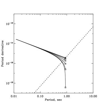
Figure 1.— $P-\dot{P}$ evolutionary diagram that shows the effect of the misalignment angle $\theta$. We show spindown trajectories for pulsars with initial period $P_{\circ}=10$ msec, magnetic field $B_{*}=10^{12}$ G, and $V_{\rm gap}=10^{13}$ Volt. Initial braking index $n=3$ is assumed ($\alpha=0$). Trajectories from bottom to top correspond to pulsars with increasing magnetic inclination angle from $0^{\circ}$ to $90^{\circ}$ with $15^{\circ}$ increments. Rectangular dots indicate when pulsars reach $P_{\rm death}$ and turn off. The dashed line represents the theoretical death line as given in eq. 15 which does not take into account the misalignment angle dependence introduced in eq. 12. Oblique pulsars evolve faster through the diagram.

3. Period Evolution and the $P-\dot{P}$ Diagram

In order to study how pulsars spin down, we equate the values of $L$ in eqs. 1 & 8 and thus obtain

$$\dot{P}=3.3\times 10^{-16}\left(\frac{P}{P_{\circ}}\right)^{2\alpha-1}\left(\frac{B_{*}}{10^{12}~{}\mbox{G}}\right)^{2}\left(\frac{P_{\circ}}{\mbox{sec}}\right)^{-1}$$

$$\times(\sin^{2}\theta+\left(1-\frac{P}{P_{\rm death}}\right)\cos^{2}\theta)$$ (12)

where from (5)

$$P_{\rm death}=8.1^{\frac{1}{2-\alpha}}\ \mbox{sec}$$

$$\times\left(\frac{B_{*}}{10^{12}\mbox{G}}\right)^{\frac{1}{2-\alpha}}\left(\frac{V_{\rm gap}}{10^{12}\mbox{Volt}}\right)^{-\frac{1}{2-\alpha}}\left(\frac{P_{\circ}}{\mbox{sec}}\right)^{-\frac{\alpha}{2-\alpha}}\ .$$ (13)

$P_{\circ}$ is the initial period at pulsar birth. Note that we have introduced an angular dependence in the definition of the death line $\dot{P}(P_{\rm death})$. As we will see below, this has interesting observational consequences. Note also that, in the limit $\theta\sim 90^{\circ}$ and $\alpha=0$, we obtain the following simple expression

$$\dot{P}_{\rm death}=5\times 10^{-18}\left(\frac{P_{\rm death}}{P_{\circ}}\right)^{3}\left(\frac{V_{\rm gap}}{10^{12}\mbox{Volt}}\right)^{2}\left(\frac{P_{\circ}}{\mbox{sec}}\right)^{3}\ ,$$ (14)

which can also be written as

$$\log\dot{P}_{\rm death}=3\log P_{\rm death}-17.3+2(\log V_{\rm gap}-12)$$ (15)

(compare with Zhang, Harding & Muslimov 2000). When $P\ll P_{\rm death}$,

$$B_{*} \propto \dot{P}^{\frac{1}{2}}P^{\frac{1}{2}-\alpha}$$ (16)

$$n = 3-2\alpha$$ (17)

$$m = n(n-1)\ ,$$ (18)

and pulsars evolve in the logarithmic $P-\dot{P}$ diagram along lines of constant magnetic field $\dot{P}\propto P^{2\alpha-1}$. As $P$ approaches $P_{\rm death}$, however, the evolution curves down away from the above straight lines and ends at a point $P=P_{\rm death}$ and $\dot{P}=\dot{P}(P_{\rm death})$ (see figure 1). This evolution is similar to what one would expect if we had assumed magnetic field decay in the standard dipole spindown model (e.g. Gonthier et al. 2002 and 2004, hereafter G02 and G04 respectively). In figure 1 we show only $\alpha=0$, or evolution with initial braking index $n=3$. For $n<3$ the straight portion of the lines would rotate counterclockwise, and would become horizontal for $n=2$ ($\alpha=0.5$). Such pulsars would also evolve faster.

As a test of the validity of our results, we tried to reproduce the observed distribution of pulsars in the $P-\dot{P}$ diagram with the minimum number of assumptions possible, through a simple Monte Carlo numerical experiment that follows G02 and G04. We integrated eq. 12 for random times $t$ within a $10^{9}$ year time interval (this mimics random pulsar birth in the galaxy). The result of the integration is recorded only if the star remains active as a pulsar, i.e. only if $P(t)\leq P_{\rm death}$. To make our results more realistic, we assumed a multipeaked lognormal distribution of polar magnetic fields around $B_{*}\sim 10^{12}\mbox{G}$ (eq. 1 in G02): $\rho_{B}=\Sigma_{i=1}^{2}A_{i}e^{-(\log B-\log B_{i})^{2}/\sigma^{2}_{i}}$. We used two terms with $A_{1}=20.0$, $A_{2}=2.0$, $\log B_{1}=12.65$, $\log B_{2}=13.0$, $\sigma_{1}=0.6$, and $\sigma_{2}=0.4$.

We assumed a uniform random distribution of initial pulse periods from 10 msec to 0.2 sec. We did account for the observational selection effect due to finite instrument detectability by implementing the radio pulsar luminosity model of Narayan & Ostriker 1990 (eqs. 23, 24 in G02), and a lower detectable pulsar luminosity limit of $12.5$ mJy$\cdot$kpc². Finally, we assumed that there is no magnetic field or misalignment angle evolution with time. In an effort to simplify the approach we did not consider the multitude of selection effects and individual survey detectability limits. We also did not calculate the distance to individual pulsars after tracking them in the galactic potential as in G02 and G04, relying on the luminosity distribution function. We believe, however, that the gross effects of the new spindown law (12) can be understood even with our procedure.

Our results are shown in figs. 2,3 & 5. In figure 2 we show the result of our simulation for the standard dipolar spindown ($\alpha=0$, or equivalently $n=3$, and no dependence on misalignment angle $\theta$, i.e., $\theta=90^{\circ}$ for all pulsars). One can directly see a strong concentration of pulsars near the death line, although the concentration is decreased by the luminosity selection effect, which favors younger brighter pulsars and fills up the upper left corner of the diagram. This concentration is understood since pulsars evolve slower and slower as they grow older. This is, however, not what is observed (figure 4). The need to make the death line boundary softer led some researchers to introduce a ”death valley” (G02) or field decay (G02, G04) in their simulations. In figure 3 we show that introducing the $\theta$ dependence that we have obtained in eq. 8 with random misalignment angles, solves this problem naturally without magnetic field decay. As we saw in figure 1 the angle-dependent death line helps in smoothing the pileup. In figure 4, we show the present day observed radio pulsar distribution from the ATNF pulsar catalog for comparison with our results. The similarity between figures 3 & 4 is quite good considering the simplifications of our model. We aim to reproduce the gross features of the observed $P-\dot{P}$ diagram for non-millisecond pulsars – its triangular shape and centroid location, while keeping the number of initial magnetic field components to a minimum. In the standard spindown picture it is very difficult to have pulsars in the lower corner of the $P-\dot{P}$ triangle without polluting the low $P$ – low $\dot{P}$ region of the diagram with low-field pulsars, which are not observed. In our spindown model the lower corner is filled with pulsars dropping from the higher $\dot{P}$ (higher $B_{*}$) region, rather than the ones moving on straight tracks as in the standard case. This contributes to the triangular shape of the diagram.

We obtain a better overall fit if we constrain the misalignment angles to be smaller than $45^{\circ}$ (figure 5). This reduces the horizontal width of the triangle, which means that more higher-field pulsars are moving on vertical tracks in the diagram. Also, the ridge of overdensity near the theoretical death line seen in figure 3 is smoothed out in figure 5.

Similar shapes of the diagram are found for $\alpha>0$. This explains individual observed pulsars with $n<3$. However, our fit deteriorates for values of $\alpha$ larger than 0.25. We thus conclude that, although individual pulsars may well have $\alpha>0$, as a whole, $\alpha\sim 0$ is a good approximation for the observed pulsar population.

Furthermore, when $\alpha=0$, from eqs. 1 & 8 we derive

$$n=3+\frac{2}{\Omega/(\Omega_{\rm death}\cos^{2}\theta)-1}\ .$$ (19)

Around the pulsar death line $\Omega\approx\Omega_{\rm death}$, this equation gives

$$n\approx 3+\frac{2\cos^{2}\theta}{1-\cos^{2}\theta}\ ,$$ (20)

which, for aligned pulsars with $\cos\theta\approx 1$ may be much greater than 3. Such high braking index values may be observable (Johnston & Galloway 1999).

In figure 6 we plot the distribution of $\cos\theta$ in our Monte Carlo simulation that was presented in figure 3. In this simulation pulsars are injected (born) with random magnetic axis orientation with respect to the rotation axis as shown by the dashed histogram in figure  6. The pulsar population at the end of the simulation, however, shows a different distribution of misalignment angles as shown by the thick solid line. The selection bias towards smaller misalignment angles may be attributed to the fact that orthogonal rotators spin down faster (on the average), and therefore are more likely to evolve beyond the death line within the observation time interval. Finally, the thin solid line represents the distribution of misalignment angles in the pulsars observed lying below the theoretical death line given by eq. 15 (which does not take into account the angle dependence introduced in eq. 12). One sees clearly that pulsars observed near or below the death line should have preferentially smaller misalignment angles $\theta$ than the rest of the pulsar population. This is, we believe, an important observational prediction of the present work.

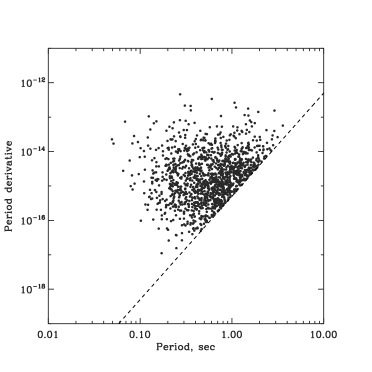
Figure 2.— Monte Carlo experiment using the standard dipole model ($\alpha=0$, or equivalently $n=3$, and no angle dependence). Pulsars are injected with a lognormal distribution of polar magnetic field values around $B_{*}=10^{12}$ G (as in G02). $V_{\rm gap}=10^{13}$ Volt. $P_{\circ}$, the initial period at pulsar birth, is uniformly randomly distributed between 10 msec and 0.2 sec. We have also introduced an observational selection effect due to finite instrument detectability limit (see text). The dashed line represents the theoretical death line as given in eq. 15. The strong concentration of pulsars near the death line is not observed in the real distribution of pulsars.

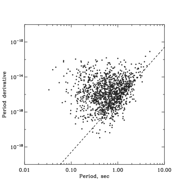
Figure 3.— Same as fig. 2, only with the misalignment random angle dependence obtained in eq. 8. The introduction of the angle dependence results in the softening of the death line.

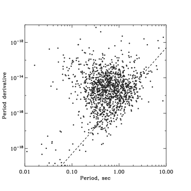
Figure 4.— The present day observed radio pulsar distribution. Data from ATNF pulsar catalog.

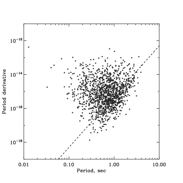
Figure 5.— Same as figure 2, but with misalignement angles constrained to be less than $45^{\circ}$.

Figure 6.— The distribution of $|\cos(\theta)|$ in our Monte Carlo experiment in figure 3. The dashed line represents the original distribution injected with uniform random misalignment angle. The thick solid line represents the distribution of misalignment angles in the simulated pulsar distribution as a whole. The thin solid line represents the distribution of misalignment angles for the pulsars observed lying below the theoretical death line given by eq. 15. An interesting observational prediction of the present work is that pulsars lying near or below the theoretical death line should have preferentially smaller misalignment angles.

Figure 7.— Distribution of alignment measure in the observed pulsar population. Each pulsar is plotted as a circle with radius proportional to the quantity $WP^{-1/2}$ using the pulse width $W$ at 50% of the peak. Data from ATNF pulsar catalog.

4. Discussion

Awaiting the development of a detailed three dimensional MHD theory for the rotating neutron star magnetosphere, we can describe a few general characteristics of its expected structure.

We argue that $\Omega_{F}$ characterizes the reduced magnetospheric electric potential drop between the magnetic axis and the edge of the open field line region. Poloidal electric currents will be generated as long as electric charges can be produced in the magnetosphere. These charges are produced in the magnetospheric polar gaps. In the axisymmetric case, $\Omega_{F}$ can also be thought as the angular velocity of rotation of open magnetic field lines, which is in general smaller than $\Omega$. The electric current that flows between the magnetic axis and the edge of the open field line region generates the spindown torque. As shown in C05, this electric current and spindown torque are both proportional to $\Omega_{F}$.

We argue that this picture describes also the situation when $\theta\neq 0$. As the neutron star rotates, the magnetic axis moves around the axis of rotation. In the rotating frame of the star, however, open field lines rotate at their own rate $\Omega-\Omega_{F}$ opposite to the direction of stellar rotation around the magnetic axis. Observational evidence for this effect can be found in the well known sub-pulse drift phenomenon (e.g. Beskin 1997; Rankin & Wright 2003). In the limit $\Omega_{F}=\Omega$, it is as if open magnetic field lines are anchored on the stellar surface. In the opposite limit $\Omega_{F}=0$, open field lines rotate around both the magnetic and rotation axes returning to the same position every rotation of the star when viewed by an inertial observer. For finite $\Omega_{F}$ a phase shift about the magnetic axis will be accumulated after every turn of the star. A simple analogy to the above picture might be that of a lawn watering system consisting of a hose rotating at angular velocity $\Omega$, and a sprinkler at its end rotating with angular velocity $\Omega_{F}-\Omega$ in the rotating frame of the watering hose.

Note that the orthogonal component does not require the establishment of a poloidal electric current circuit in order for it to slow down the stellar rotation. The orthogonal component emits spiral electromagnetic waves (in general Alfven waves) which travel out to infinity through the rotating or non-rotating open field lines.

The main conclusions of the present work are:

1. The electromagnetic energy loss of a pulsar depends not only on the surface magnetic field $B_{*}$ and on the rotational angular velocity $\Omega$, but also on the misalignment angle $\theta$ and on the angular velocity of the open magnetic field lines $\Omega_{F}$ (which is in general smaller than $\Omega$).

2. The approach to pulsar death modifies the rate of energy loss. The death occurs when the pulsar slows down sufficiently so that the angular velocity of the open fieldlines $\Omega_{F}=0$.

3. The energy loss close to the pulsar death is smaller than what is given by the standard dipolar spindown formula. This effect gives a good fit between the theoretical and observed distributions of pulsars near the death line, without invoking a magnetic field decay.

4. Our model may also account for individual pulsars spinning down with braking index $n<3$. However, $n\sim 3$ remains a good approximation for the pulsar population as a whole.

5. Pulsars near the death line have braking index values $n>3$. Such high braking index values may be observable.

6. Pulsars near the death line may have preferentially smaller inclination angles.

A preliminary look at the ATNF pulsar catalog data suggests that the last point may have some observational support. One possible measure of the inclination angle of a pulsar is its fractional pulse width, or the ratio of the width of the pulse to the period of the pulsar. If the radio beam size is independent of inclination, then we would expect pulsars with smaller inclinations to be seen for a larger fraction of the period than pulsars with large inclinations. In order to test this hypothesis we took the available data for the pulse width at 50$\%$ of the pulse peak from the ATNF catalog (1375 pulsars with $W_{50\%}\neq 0$). In order to be able to compare the fractional pulse width for pulsars of different periods, we have to correct for the intrinsic size of the pulsar beam. If the beam roughly follows the angular size of the open fieldlines, then the beam size falls as $P^{-1/2}$ with increasing period (we are assuming that the last closed field line extends out to the light cylinder). Therefore, the quantity that should relate to the degree of alignment is $F_{\rm align}\equiv(W\times P^{1/2})/P=WP^{-1/2}$, where $W$ is the measured pulse width. In figure 7 we plot the observed pulsars as circles with the radius of the circle linearly proportional to $F_{\rm align}$. A visual inspection of the plot shows that there is an excess of larger pulse fractions for older pulsars, and in particular for pulsars near the right edge of the $P-\dot{P}$ triangle. This region is near the pulsar death line (dashed line), and therefore, this feature is particularly interesting. Obviously, a much better analysis needs to be performed, but these results are quite encouraging. An overabandunce of pulsars with large pulse fractions near the death line in a smaller pulsar sample had also been interpreted by Lyne and Manchester (1988) as an indication of alignment.

In an effort to simplify the fits we have assumed in this paper that the misalignment angle stays the same during the evolution, and there is no field decay. The reality may of course be more complicated, and there could be some amount of field decay, and potential alignment (and consequent precession) during the lifetime of a pulsar, due to electromagnetic torques on the star. These effects would introduce extra degrees of freedom to fitting the pulsar distribution. We hope, however, that the physically motivated spindown law of the type introduced in this work would find its way into detailed population synthesis models.

Appendix A Appendix A: Calculation of Open Magnetic Flux

We present here expressions for $\psi_{\rm open}(r_{c})$ obtained numerically for various axisymmetric magnetospheric configurations using the numerical code developed in C05:

• Standard magnetostatic dipole:

  $$\psi_{\rm open}=\frac{B_{*}r_{*}^{3}}{2r_{c}}\ .$$ (A1)

  Note that in this limit, $\psi_{\rm open}(r_{c})$ is defined as the amount of flux that crosses the equator beyond equatorial distance $r_{c}$. All field lines cross the equator perpendicularly.

• Magnetostatic dipole with open field lines beyond $r_{c}$:

  $$\psi_{\rm open}=1.20\frac{B_{*}r_{*}^{3}}{2r_{c}}\ .$$ (A2)

  Note that this implies the existence of an equatorial azimuthal current sheet beyond $r_{c}$. The magnetosphere is otherwise stress-free. The last open field lines crosses the equator at an angle of about $70^{o}$ towards the axis (‘Y’ point).

• Rotating (relativistic) dipole with open field lines beyond $r_{c}$, and smooth crossing of the light cylinder:

  $$\psi_{\rm open}=1.23\frac{B_{*}r_{*}^{3}}{2r_{c}}\ .$$ (A3)

  This result is valid for $r_{*}\ll r_{c}\leq r_{lc}$. The solution requires the presence of a) a poloidal electric current along open field lines, b) a poloidal current sheet along the separatrix between open and closed field lines, and c) an equatorial azimuthal current sheet beyond $r_{c}$. The last open field line crosses the equator at an angle of about $70^{o}$ towards the axis. Note the interesting similarity with the latter non-relativistic case (eq. A2).

Appendix B Appendix B: Calculation of $\Omega_{F}$

We derive here an approximate expression for $\Omega_{F}$, assuming $\Omega_{F}=\mbox{const}$. We perform the calculation in the aligned (axisymmetric) case $\theta=0$. It has been shown in C05 that $\Omega_{F}$ is related to the magnetospheric potential drop $V_{F}$ between the magnetic axis (characterized by $\psi=0$) and the edge of the open field line region (characterized by $\psi=\psi_{\rm open}$), namely

$$V_{F}=\int_{\psi=0}^{\psi_{\rm open}}{\bf E}\cdot{{\rm d}{\bf s}}=\int_{\psi=0}^{\psi_{\rm open}}\frac{s\Omega_{F}}{c}B_{p}{\rm d}s=\frac{1}{c}\int_{\psi=0}^{\psi_{\rm open}}\Omega_{F}{\rm d}\psi$$

$$=\frac{\Omega_{F}\psi_{\rm open}}{c}\ ,$$ (B1)

where $s$ is the distance from the rotation axis; ${\bf E}$ is the electric field; $B_{p}$ is the poloidal (meridional) component of the magnetic field. $V_{F}$ is in general different from the corresponding stellar potential drop, namely

$$V_{*}=\frac{1}{c}\int_{\psi=0}^{\psi_{\rm open}}\Omega{\rm d}\psi=\frac{\Omega\psi_{\rm open}}{c}\ .$$ (B2)

The difference

$$V_{\rm gap}\equiv V_{*}-V_{F}=\frac{(\Omega-\Omega_{F})\psi_{\rm open}}{c}$$ (B3)

is just the particle acceleration gap potential which devolops along the magnetic field near the footpoint of open field lines (e.g. Beskin 1997). Therefore,

$$\Omega_{F}=\Omega-\Omega_{\rm death}\ ,$$ (B4)

where

$$\Omega_{\rm death}\equiv\frac{V_{\rm gap}}{\psi_{\rm open}}c\ .$$ (B5)

This expression is valid as long as $\Omega\geq\Omega_{\rm death}$. When $\Omega<\Omega_{\rm death}$, $\Omega_{F}=0$.

References

- Alvarez, Carramiñana (2002) Alvarez & Carramiñana 2004, A&A, 414, 651
- Beskin (1997) Beskin, V.S. 1997, Physics-Uspekhi, 40, 659
- BlandfordRomani (88) Blandford R. D. & Romani R. W. 1988, MNRAS, 234, 57
- Contopoulos, Kazanas, Fendt (1999) Contopoulos, I., Kazanas, D. & Fendt, C. 1999, ApJ, 511, 351 (CKF)
- Contopoulos (05) Contopoulos, I. 2005, A&A, 442, 579 (C05)
- Goldreich & Julina (1969) Goldreich, P. & Julian, W. H. 1969, ApJ, 157, 869
- Gonthier et al (2002) Gonthier, P. L., Ouellette, M. S., Berrier, J., O’Brien, S. & Harding, A. K. 2002, ApJ, 565, 482 (G02)
- Gonthier et al (2004) Gonthier, P. L., Van Guilder, R. & Harding, A. K. 2004, ApJ, 604, 775 (G04)
- Gruzinov (2005) Gruzinov A. 2005a, Phys. Rev. Lett., 94, 021101
- (10) Gruzinov A. 2005b, astro-ph/0502554
- Harding, Contopoulos & Kazanas (1999) Harding, A. K., Contopoulos, I. & Kazanas, D. 1999, ApJ, 525, 125
- Hibschman & Arons (2001) Hibschman, J. A. & Arons, J. 2001, ApJ, 554, 624
- (13) Johnston, S. & Galloway, D. 1999, MNRAS, 306L, 50
- (14) Lyne, A. G. & Manchester, R. N. 1988, MNRAS, 234L, 477
- Mestel (1999) Mestel, L. 1999, ”Stellar Magnetism”, Oxford University Press
- (16) Narayan R. & Ostriker J. P. 1990, ApJ, 352, 222
- Rankin & Wright (2003) Rankin, J. M. & Wright, G. A. E. 2003, A&A Rev., 12, 43
- Timokhin (2005) Timokhin, A. 2005, astro-ph/0507054
- (19) Zhang B., Harding A. K., Muslimov A. G., 2000 ApJL, 531, 135