MOJAVE: Monitoring of Jets in AGN with VLBA Experiments - II. First-Epoch 15 GHz Circular Polarization Results

Abstract

We report first-epoch circular polarization results for 133 active galactic nuclei in the MOJAVE program to monitor the structure and polarization of a flux limited sample of extra-galactic radio jets with the VLBA at 15 GHz. We found strong circular polarization ($\geq 0.3$%) in approximately 15% of our sample. The circular polarization was usually associated with jet cores; however, we did find a few strong jet components to be circularly polarized. The levels of circular polarization were typically in the range of $0.3-0.5$% of the local Stokes-$I$. We found no strong correlations between fractional circular polarization of jet cores and source type, redshift, EGRET detections, linear polarization, or other observed parsec-scale jet properties. There were differences between the circular-to-linear polarization ratios of two nearby galaxies versus more distant quasars and BL Lac objects. We suggest this is because the more distant sources either have (1) less depolarization of their linear polarization, and/or (2) poorer effective linear resolution and therefore their VLBA cores apparently contain a larger amount of linearly polarized jet emission. The jet of 3C 84 shows a complex circular polarization structure, similar to observations by Homan & Wardle five years earlier; however, much of the circular polarization seems to have moved, consistent with a proper motion of 0.06$c$. The jet of 3C 273 also has several circularly polarized components, and we find their fractional circular polarization decreases with distance from the core.

Accepted for Publication in the Astronomical Journal

1 Introduction

Only a small fraction of the radio emission from extra-galactic radio jets associated with Active Galactic Nuclei (AGN) is circularly polarized; however, this weak component is a potentially important probe of the particle population and magnetic field structure of the jets. Circular polarization (CP) can be produced either as an intrinsic component of the emitted synchrotron radiation, or via Faraday conversion of linear polarization into circular (Jones & O’Dell, 1977). If the intrinsic mechanism dominates, jets must be a predominantly electron-proton plasma and must contain a significant fraction of unidirectional ordered magnetic field. If the conversion mechanism dominates, circular polarization probes the low energy end of the relativistic particle distribution (e.g. Wardle & Homan, 2003), a key parameter in studying the bulk kinetic luminosity of AGN jets and their particle content (Celotti & Fabian, 1993; Wardle et al., 1998). Faraday conversion is expected to be the dominant mechanism on theoretical grounds (e.g. Jones, 1988); however, there is still only limited observational evidence supporting this view (Wardle et al., 1998; Homan & Wardle, 2004).

Early integrated measurements of CP from AGN jets (Weiler & de Pater, 1983; Komesaroff et al., 1984) revealed circular polarization to be only a very small fraction, typically $<0.1$%, of their total flux. However, the Very Long Baseline Array (VLBA), has made it possible to study circular polarization from extragalactic jets at sub-milliarcsecond resolution. Wardle et al. (1998) and Homan & Wardle (1999, hereafter HW99) found circular polarization in cores of four powerful AGN jets at local fractional levels of $0.3$ to $1$% of Stokes-$I$ with the VLBA. Circular polarization has since been detected with various instruments in other AGN jets (Rayner et al., 2000; Homan et al., 2001) and a wide variety of other synchrotron emitting sources: low-luminosity AGN such as Sagittarius A* and M81* (Bower, Falcke, & Backer, 1999; Sault & Macquart, 1999; Brunthaler et al., 2001; Bower, Falcke, & Mellon, 2002), intra-day variable sources (Macquart et al., 2000), and galactic micro-quasars (Fender et al., 2000, 2002).

Despite the detection of the circular polarization in a variety of sources, observations of circular polarization from AGN jets are fragmented and incomplete. A large temporal gap exists between the integrated measurements of the 1970’s to early 1980’s and the high resolution VLBA measurements from the mid 1990s onward. Only a few AGN jets have high resolution, multi-epoch circular polarization observations that are matched in observing frequency and sensitivity. An even smaller number of sources have multi-frequency circular polarization observations suitable for measuring a spectrum. Additionally, the small, ad hoc samples studied to date have not allowed for an analysis of correlations between the appearance of strong circular polarization and other source properties. While these previous studies raised a number of interesting possibilities of how circular polarization could be used to constrain the magnetic field properties and particle populations of AGN jets, a systematic survey of a large complete sample is necessary to make further progress.

We have exploited the VLBA’s unique imaging capabilities by studying the milliarcsecond-scale circular polarization of a complete AGN jet sample at 15 GHz as part of the MOJAVE (Monitoring Of Jets in AGN with VLBA Experiments) program. The MOJAVE sample of 133 AGN is complete and flux limited on the basis of VLBA-scale emission. The selection criteria are described in detail in Lister & Homan (2005) which also reports first-epoch linear polarization results; however, in brief, for inclusion in MOJAVE, a source must have had a total 15 GHz VLBA flux density of at least 1.5 Jy ($>2$ Jy for sources south of the celestial equator) at any epoch from 1994–2003. When completed, MOJAVE will have obtained at least four epochs of full Stokes VLBA images at 15 GHz of all sources in the sample. In addition, multi-frequency follow-up programs will study the circular polarization spectrum of the strongly circularly polarized sources identified by MOJAVE.

In this paper, we report only the first-epoch circular polarization results from the MOJAVE program. Future papers will explore other aspects of this rich data set including multi-epoch circular polarization variability. The details of our observations and calibration appear in section 2. We present and discuss our results in section 3, and our conclusions appear in §4.

2 Observations and Calibration

Each MOJAVE observing session targets 18 sources over a 24 hour period, and this paper presents results drawn from the first eleven sessions, from 2002 May 31 through 2004 February 11. During each 24 hour session, observations of the 18 sources are broken up into highly interleaved scans, each approximately seven minutes in duration. The schedule is designed to maximize coverage in the $(u,v)$-plane; however, as discussed below, the highly interleaved nature of the observations also improves our ability to calibrate the antenna gains to detect circular polarization. We observed each source for approximately 65 minutes of total integration time. No additional calibrators were observed as all of our target sources were strong and compact.

The data were recorded at each VLBA antenna at a central observing frequency of 15.366 GHz using 1-bit sampling and were correlated at the VLBA correlator in Socorro, NM. The correlator output was 2 s integrations for all four cross-correlations (RR, RL, LR, LL). The correlated data contained four intermediate frequencies (IFs) and 16 channels per IF, yielding a total bandpass of 32 MHz in both RR and LL. Tapes of the correlated data were shipped to NRAO in Charlottesville, VA and Purdue University where they were loaded into NRAO’s Astronomical Image Processing System (AIPS) for further processing.

The basic calibration procedure followed the standard methods outlined in the AIPS cookbook and the procedure by HW99 for measuring circular polarization with the VLBA using the gain transfer technique. Below we briefly describe our basic calibration procedure, in §2.1 we discuss some improvements to the gain transfer procedure developed for these observation, and in §2.2 we discuss some checks on our calibration procedure.

The data were loaded into AIPS using the VLBALOAD procedure. The procedure VLBACALA was then used to do a-priori amplitude calibration, running both the ACCOR and APCAL tasks, including an atmospheric opacity correction. The parallactic angles were removed using the procedure VLBAPANG and the pulse calibration was applied using VLBAPCOR. The procedure VLBAFRNG was then used to perform fringe fitting. All of our sources were strong enough to serve as their own fringe calibrator, and no special interpolation from strong to weak sources was necessary. We used the procedure CRSFRING to remove any residual multi-band delay difference between the right and left-hand systems of the array. Finally we ran BPASS to apply a bandpass correction before averaging across the channels within each IF and ’splitting’ the data off into individual source files.

Following a 2 s time-scale point-source phase calibration to increase coherence, the data were written out to the CALTECH VLBI program, DIFMAP (Shepherd, 1997). In DIFMAP, the data were averaged to 30 seconds and edited in a station-based manner. An edited version of the data was then saved without any self-calibration applied. We will refer to this version of the data as the edited/unself-calibrated data. Normal self-calibration and imaging techniques were then used within DIFMAP to obtain the best Stokes-$I$ model for each source.

For each source, the best Stokes-$I$ model and the edited/unself-calibrated data were then read back into AIPS, and the data were self-calibrated against the model using the task CALIB in amplitude and phase (SOLMODE = ’A&P’) on a 30 second timescale. The antenna feed-leakage term corrections from LPCAL (see below) were applied using SPLIT and the parameter DOPOL = 3 to guarantee that the corrections were applied to both the parallel and cross-hand correlations. A final pass of CALIB self-calibrated the data again against the Stokes-$I$ model to remove any errors by the initial self-calibration prior to D-term removal. For circular polarization calibration via gain transfer it is important that both passes of CALIB described above were performed only making the rigorous assumption that $(RR+LL)/2=I_{model}$. This left as un-calibrated any gain offsets between the right (R) and left (L) hand feeds at each antenna. The gain transfer calibration described in §2.1 was used to remove these offsets. After correction of the $R/L$ antenna gains, final images were made in all four Stokes parameters.

It is important to note that the antenna feed leakage corrections were initially determined on each source individually using LPCAL, and the final corrections (which were applied to the data) were determined by taking the median of these after removing obvious outliers. Our typical feed leakage terms (D-terms) had amplitude of about 0.02 with the largest being 0.05, and we estimate that we have made these corrections accurate to about $\pm 0.005$ . Following HW99, we estimate any uncertainty in our fractional circular polarization measurements, $m_{c}$, due to leakage correction errors to be of the order $\Delta m_{c}<0.001m_{L}+1\times 10^{-5}$, where $m_{L}$ is the fractional linear polarization of the map peak (typically a few percent or less). Thus any uncertainty due to leakage feed corrections is very much smaller than the uncertainty due to the gain calibration and can be neglected.

2.1 R/L Gain Calibration

As described in HW99 and Homan et al. (2001), the gain transfer technique requires that we initially make no assumption about circular polarization during self-calibration, i.e., we only assume $(RR+LL)/2=I_{model}$ as discussed above. This will leave as un-calibrated a small relative R/L complex gain ratio at each VLBA antenna. The essential idea is to calibrate this gain ratio with a smoothed set of R/L complex antenna gains determined from all 18 sources in each 24 hour observing session.

To determine the smoothed set of antenna gains that will ultimately be applied to the data, we first solve for the R/L complex gain ratios by self-calibrating each source assuming no circular polarization in that source ($RR=I_{model}$ and $LL=I_{model}$). These solutions are not applied to the data, but rather they are collected into a single calibration table which we smooth by using a six-hour running median with all sources equally weighted. Solutions from sources with low gain SNR or very strong circular polarization (greater than 0.5%) are prevented from contributing to the running median. To account for the possibility of smaller levels of real circular polarization showing up in the raw R/L antenna gains of individual sources, we subtract from the raw R/L gain ratios for each source a single mean offset (taken across all times, antennas, and IFs for that source) from the running median. The sum of the applied offsets for all sources in a given 24 hour observing session is constrained to be zero. This constraint guarantees quick convergence of an iterative algorithm which generates a trial set of smoothed gains, computes mean offsets for each source, takes those offsets out of the data, and then repeats the process. The constraint also underscores the fundamental assumption of the gain transfer technique: that any single observing session will have an average circular polarization of zero across all the sources in the sample. This assumption may introduce a small overall gain bias in any individual epoch; however, our Monte Carlo method of estimating the uncertainty due to the gain calibration (described below) naturally accounts for this possibility.

We note that the procedure described above for accounting for sources with small levels of real circular polarization differs from the procedure used in HW99 and Homan et al. (2001). In those papers, we prevented such sources from contributing to the smoothed gains through an iterative process where the strongest polarized sources were removed first, the smoothed gains recomputed, and the process repeated until no source contributing to the smooth gains appeared to have real circular polarization. In those papers, we found the final results were insensitive to the detailed steps of this process; however, the process was time consuming and difficult to automate. For the MOJAVE program, we needed a procedure that was automated, reproducible, and could be easily tested by a Monte Carlo simulation we developed. As a check that the new procedure gave the same results as our previous methods, we reprocessed the antenna gain solutions from the 40 source observation analyzed in Homan et al. (2001). For the circularly polarized sources in that experiment, we found an RMS R/L gain difference of $0.017$% between our technique and the original. This difference is approximately one-third of the estimated gain uncertainty of that experiment, verifying that the two techniques indeed give effectively the same results.

2.1.1 Uncertainty in Measured CP due to Gain Transfer

In the appendix of Homan et al. (2001), we laid out a prescription for estimating the uncertainty in circular polarization measurements made by gain transfer. Here we improve on that work by using a Monte Carlo simulation to test our methods and obtain more accurate uncertainty estimates. As in Homan et al. (2001), we focus on amplitude gain errors, as those dominate the uncertainty in the technique. Phase errors will not contribute to first order for point-like sources, and for sources with significant extended structure, phase errors will produce anti-symmetric structure around the phase center. In section §2.2 we discuss possible phase effects and tests to constrain/resolve those issues.

The Monte Carlo simulation we developed generates 18 point sources (Most sources in our sample are dominated by a point source, e.g., Lister & Homan (2005).), and for each source generates a circular polarization with magnitude drawn at random from the distribution of observed mean gain offsets in the real gain table. The sign ($+$ or $-$) of the CP signal for each source is determined at random. Finally, a Gaussian deviate representative of our measurement uncertainty is added to each value. Each of these generated CP values is then stored for comparison to the “measured” value at the end of a Monte Carlo trial.

To generate the gain table for the simulation, a random slowly-varying gain curve is created for each antenna/IF with amplitudes and timescales similar to those in the real gain curves. To this slowly-varying gain curve is added randomly-generated scan-to-scan variations of the same range of amplitudes as seen for the corresponding source in the real gain table. Finally, the generated CP values are added to the gain curves as offsets for each source. This step is important to mimic the real gain table, which was generated from the assumption that each source has no circular polarization, so the real raw gain table contains ’corrections’ to the circular polarization of each source in addition to the actual gain variations.

Finally, this randomly-generated ’raw’ gain table is processed by exactly the same procedure we used on the real gain curve. A smoothed version of the raw table is produced by our standard procedures and compared with the raw gain table. If the procedures work correctly, the only differences between the raw and smoothed tables should be the circular polarizations set at the beginning of the simulation trial. Therefore, by comparing the two tables, we can estimate the uncertainty due to the gain calibration procedure. We repeat this simulation for 1000 independent trials to generate an estimate of the uncertainty for each source.

To safe-guard against the possibility that an unusual combination of circularly polarized sources in our data has made our results more uncertain than the above simulation indicates, we also ran a second version of the Monte Carlo described above. The only difference is that the initial circular polarization of each source in the simulation is forced to match the mean gain offset of the corresponding source in the real gain table (plus a Gaussian deviate to represent measurement uncertainty). To these values, we add a randomly-determined overall bias (the same for all 18 sources) to account for the possibility that the circular polarizations in the sample do not average to zero. The size of this gain bias is determined from the RMS of the mean offset values in the real gain table. The larger of the uncertainties from the first and second version of the Monte Carlo simulations are used to represent the total gain uncertainty for a given source; however, in practice the two Monte Carlo simulations give very nearly the same estimate of uncertainty.

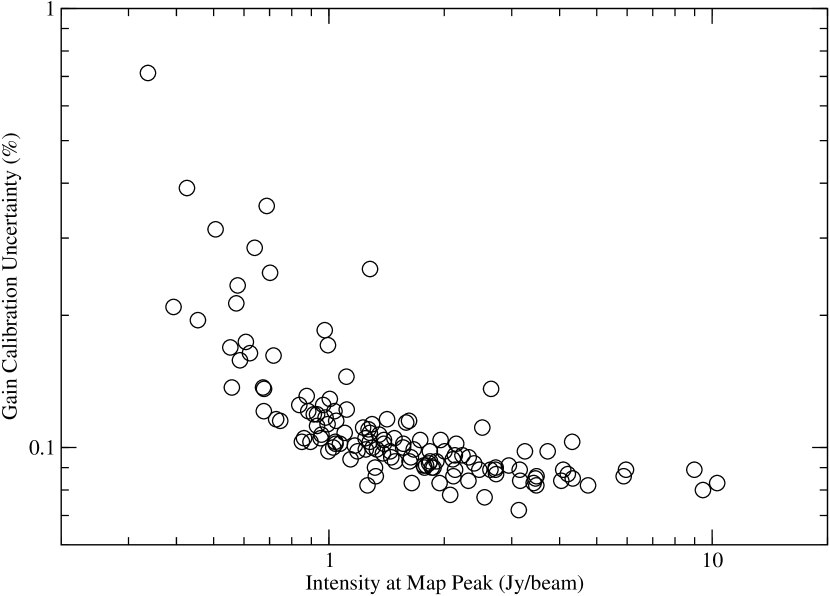
Figure 1: Gain calibration uncertainty for circular polarization (as a percentage of Stokes-$I$) as a function of Stokes-$I$ intensity at the map peak for the 133 sources in our sample.

Figure 1 shows a plot of uncertainty in fractional circular polarization measurements due to gain calibration as a function of the peak Stokes-$I$ flux for the 133 sources in the MOJAVE sample. The trend of larger uncertainties for weaker sources is expected and is driven by the larger self-calibration gain uncertainties in the weaker sources; however, it will be important to consider this trend when interpreting the results in §3. Note that most sources in the sample have uncertainty contributions from gain calibration very close to 0.1%, and given that the gain uncertainties dominate the total uncertainty (the much smaller RMS map noise is added in quadrature), our procedures are able to robustly detect CP signals as small as 0.3% of the Stokes-$I$ peak at the 3-$\sigma$ level.

2.2 Phase Calibration for Circular Polarization

Because there is no phase connection between sources in our sample (they are well separated in the sky and fringe-fit separately), the gain calibration technique described above is only effective for calibrating the antenna amplitude gains. We do allow the possibility of a phase correction in the gain transfer technique (the median phase difference between the right and left hands is treated in a similar fashion to the median amplitude ratio.); however the applied corrections are generally $\lesssim 0.1$ degrees for each antenna/IF combination.

For effective relative R/L phase correction at each antenna we rely first on the pulse calibration corrections, then on fringe fitting and the initial phase calibration in CALIB to increase coherence before averaging the data in time in DIFMAP. Each of these steps provides separate phase corrections for the left and right-hand feeds at each antenna. The pulse calibration makes no assumptions about circular polarization in the source; however both fringe fitting and the initial phase calibration to increase coherence make their corrections assuming the source is point-like. Any real circular polarization on a point source will not appear as a gain error in the antenna phases (HW99), so for most sources in our sample phase corrections found in this fashion will remove only genuine R/L phase gain errors from the data.

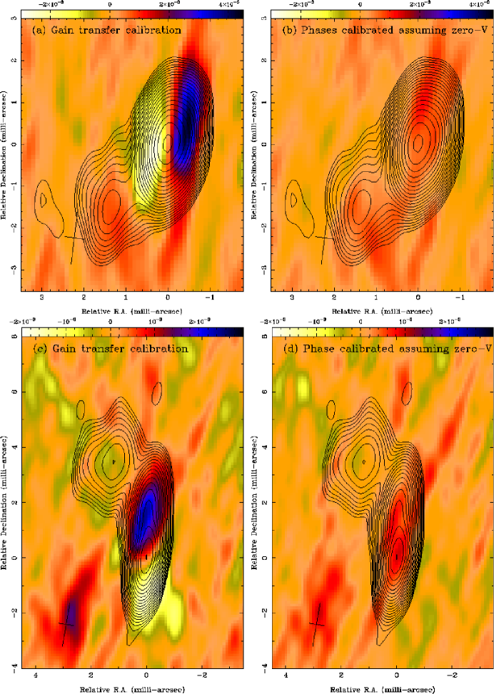
Figure 2: Circular polarization (color-scale given in mJy beam^-1) superimposed on Stokes-$I$ contours for 1213$-$172 (top panels) and 2243$-$123 (bottom panels). The $I$ contours start at 1 and 2 mJy beam^-1 respectively for 1213$-$172 and 2243$-$123 and increase in steps of $\times\sqrt{2}$. The FWHM dimensions of the restoring beams are indicated by a cross in the lower left corner of each panel. Left hand panels (a,c) show the results of straight gain transfer calibration which has a combination of real circular polarization plus phase errors. Right hand panels (b,d) show the additional effect of a round of phase self-calibration assuming no circular polarization in the data. For both sources, the additional phase calibration has corrected a phase shift in the data between the left and right hand data, and reveal that the source has no real circular polarization.

If a source has significant extended structure in Stokes-$I$, the right and left hand systems of the array may receive slightly different solutions in the algorithm’s attempt to find point source solutions to the right and left hand data separately. Most likely this will generate a small difference in the phase centers of the right and left hand data. While this small difference will not affect the Stokes-$I$ image, it may be enough to generate an anti-symmetric stripe of circular polarization across the strongest parts of the source. The effect is only apparent in the circular polarization image because Stokes-$V$ is formed by taking the difference of the right and left hand data ($V=(RR-LL)/2$), whereas Stokes-$I$ is formed from their average. See panels (a) and (c) of Figure 2 for examples of this effect.

To account for this effect and other possible phase errors in our data, we have generated two circular polarization images of each source. The first image is generated from the gain transfer calibration alone and may contain unaccounted-for phase errors. The second image is generated after an additional round of self-calibration of the phases alone. During this self-calibration of the phases, we assume there is no circular polarization in the data so both the $RR$ and $LL$ data are compared to $I_{model}$ to find the antenna phase corrections for the right and left-hand feeds separately. This self-calibration will very effectively remove any genuine R/L phase gain errors remaining in the data, as shown in panels (b) and (d) of Figure 2. The large majority of the sources in our sample are core-dominated and thus show no significant differences between the images produced before and after this phase self-calibration; however, an important minority of sources with significant extended structure do show differences (usually both in their noise levels and in their apparent circular polarization) between the two sets of images.

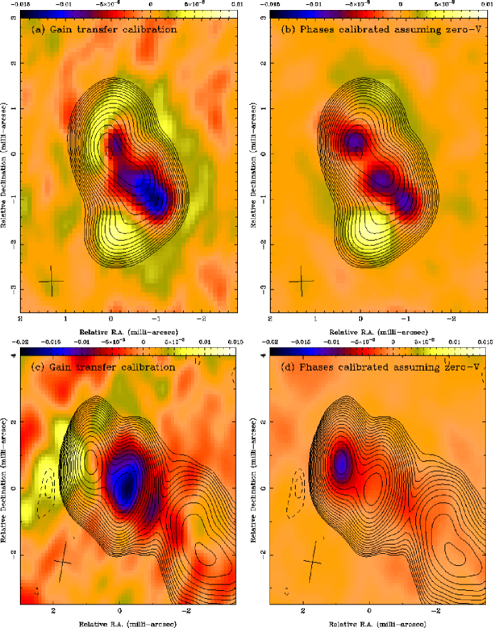
Figure 3: Circular polarization (color-scale given in mJy beam^-1) superimposed on Stokes-$I$ contours for 3C 84 (top panels) and 3C 273 (bottom panels). The $I$ contours for both sources start at 10 mJy beam^-1 and increase in steps of $\times\sqrt{2}$. The FWHM dimensions of the restoring beams are indicated by a cross in the lower left corner of each panel. Left hand panels (a,c) show the results of straight gain transfer calibration which has a combination of real circular polarization plus phase errors. Right hand panels (b,d) show the additional effect of a round of phase self-calibration assuming no circular polarization in the data. For 3C 84, panel (b), the additional phase calibration has corrected the phase errors and revealed the circular polarization of the source in greater detail, although the main features appear quite similar to panel (a). For 3C 273, panel (d), the additional phase calibration has corrected the phase error and reveals that the real circular polarization in the source is on the jet core and not on the jet component. Note that the images shown here for 3C 273 are from our second MOJAVE epoch on this source (August 28, 2003), but they are included here as an illustrative example.

Figure 3 illustrates two cases where the antenna phase errors have been removed to reveal real circular polarization. It is important to know to what extent (if any) the resulting circular polarization in these images has been modified by the phase calibration assuming zero circular polarization. In general, phase differences between RR and LL due to real circular polarization do not show up in a consistent antenna-based fashion (as would phase gain errors); however it is possible that some combination of antenna-based phase gains could be found by the self-calibration algorithm which minimizes these real phase differences and thus modifies the real circular polarization of the source.

We have tested for this effect by (1) removing all circular polarization from a real source (by setting $RR=LL=I$), (2) adding known amounts of circular polarization, and then (3) self-calibrating the phases of that data assuming no circular polarization. We have done this for several sources from our observations, and in general we find that the known circular polarization is not modified very much by this procedure. We usually see some reduction in amplitude from a few percent up to about 10% of the known CP value, and the location of the CP peak may be shifted a fraction of a beam-width to better align with the map peak (assuming it is near the map peak to begin with). In some sources with a broad core-region (core $+$ barely resolved component), a single component of CP is spread out by this self-calibration to encompass the whole region. Large shifts in CP location (more than a half a beam-width) or large reductions in amplitude (more than 20%) do not seem possible with this procedure. For example, our tests on the images in Figure 3 show that real circular polarization that began on the first jet component would remain there after phase self-calibration and would not be shifted to the core; thus, we can be confident that the real circular polarization in this epoch of 3C 273 is actually associated with the core as revealed in panel (b).

3 Results and Discussion

Our first-epoch circular polarization measurements are summarized in Tables 1, 2, and 3. Table 1 lists the linear and circular polarization measurements at the peak of each map. In most cases the Stokes-I map peak corresponds to the unresolved VLBI core; however, in a handful of cases the core and map peak do not coincide. In most of these cases, the peak appears at the location of a strong component within the jet, and we take the core to be the compact component at the base of the jet. The core of 0923$+$392 is taken at the location identified by Alberdi et al. (1993). The core of 0316$+$413 (3C 84) is a special case and is discussed further in §3.3. The off-peak jet cores are listed in Table 2, along with measurements of their linear and circular polarization at the core location. Table 3 lists the circular polarization measured on all jet components in our sample with peak fluxes stronger than 300 mJy beam^-1. We chose 300 mJy beam^-1 as a reasonable cutoff for the jet component analysis as our typical uncertainty levels would still allow very strong circular polarization of $m_{c}=0.5$% to be detected on such a component.

The linear polarization was always measured at the location of the Stokes-I peak (or at the location of the VLBI core or jet component in the cases of Tables 2 and 3 respectively). Limits are given for the linear polarization when the measured value does not exceed five times the map RMS noise. Circular polarization was also measured at the location of the Stokes-I peak (or at the location of the VLBI core or jet component for Tables 2 or 3) unless there was a CP peak within two pixels of the Stokes-I measurement location. In that case, the value of the CP peak was used instead. This procedure was used because with our phase calibration (see section 2), there may be a small positional shift in the location of the circular polarization relative to the Stokes-I. The raw circular polarization measurements and their uncertainties are given in Tables 1, 2, and 3. The uncertainties includes both the gain transfer uncertainty from our Monte Carlo simulation (see §2) and the RMS noise added in quadrature. It is important to note that the fractional circular polarization values reported in the Tables include both measurements and limits. While we do actually measure a CP value in every case, most of these measurements are not significant, and thus we have chosen a $2\sigma$ cutoff, below which we report a limit on the value of $|m_{c}|$. The quoted limits on $|m_{c}|$ are the larger of $\left(|\mathrm{V}|+1\sigma_{\mathrm{V}}\right)$ or $2\sigma_{\mathrm{V}}$. The raw values of $m_{c}$ in the cases that are less significant than $2\sigma_{\mathrm{V}}$ can be computed from the $V$ and $I$ intensities reported in the Tables.

We note that we have applied exactly the same procedures to the cores and jet components in Tables 2 and 3 as we applied to the map peak values; and, as argued in §2.1, the interpretation of the gain uncertainties is most robust for the map peak. Therefore, we are somewhat less confident of the uncertainties reported in Tables 2 and 3; however, we believe that the gain uncertainties will still accurately account for the possibility of any overall gain bias in the CP map. The gain uncertainties do not account for the possibility of random (but not net) gain errors creating small amounts of spurious circular polarization off the map peak; however, the RMS noise level in the map naturally takes this into account. We notice no particular trend for map noise to be scattered preferentially onto weaker source structure, and we therefore believe that the combination of gain uncertainties and map RMS noise provides a reasonable uncertainty estimate for the off-peak circular polarization reported in Tables 2 and 3.

3.1 Circular Polarization on VLBI Cores

Figure 4 shows the distribution of core circular polarization for all the sources in our sample. For the purposes of this figure we use measured values rather than limits in every case. We detect circular polarization in 17 out of 133 jet cores at the $3\sigma$ level or higher significance. Of the 115 sources with overall uncertainties less than $0.15$%, we measure circular polarization stronger than $0.3$% of the local Stokes-I in 17 of those sources (all but two of those at $\geq 3\sigma$ significance). The existence of strong circular polarization ($\geq 0.3$%) in about 15% of our sample is somewhat higher than the rate of strong circular polarization observed by Homan et al. (2001) with the VLBA at 5 GHz. They found CP stronger than 0.3% in only 2 out of 36 sources (6%); however, these rates of strong circular polarization detection are compatible according to Poisson statistics.

We examined the circular polarization distribution between source types (using the optical classifications given by Lister & Homan, 2005), and a Gehan’s Generalized Wilcoxon test from the ASURV package (Lavalley et al., 1992) shows no significant difference between the distributions for quasars and BL Lac objects. Unfortunately there are simply too few galaxies in the MOJAVE sample for a robust test of their distribution. A Gehan’s test also shows no significance difference between the EGRET and non-EGRET detected sources (as defined in Lister & Homan, 2005) in terms of their CP levels.

Due to the large number of limits in our sample, we used a Kendall-Tau test for censored data (Lavalley et al., 1992) to test for correlations between circular polarization and various other source properties. Table 4 collects the results of these tests. The Kendall-Tau test gives the probability that no correlation exists between fractional circular polarization, $|m_{c}|$, and the property in question. Small values in the Table indicate that a correlation may exist, and we take $p<0.05$ as suggestive of a correlation. Of the twenty properties tested in Table 4, we find only three with $p\lesssim 0.05$: 15 GHz jet flux ($S_{jet}$), 15 GHz core/jet flux ratio ($R_{jet}$), and 15 GHz core/total flux ratio ($R_{total}$) as defined by Lister & Homan (2005). These three properties are closely related through the prominence of the VLBI scale jet, so we really only have one property with a possible correlation at the $p<0.05$ level, consistent with pure chance. Removing 3C 273 from consideration raises $p$ to $0.12$ for $S_{jet}$ and $0.09$ for $R_{total}$, so we don’t find strong evidence that circular polarization is correlated with any of these properties.

While Galactic latitude, $|b|$, is not correlated with circular polarization, it is interesting that of the 12 sources near the galactic plane ($|b|<10$ degrees), none of them have circular polarization at $\geq 2\sigma$. Treating these sources and those with $|b|>10$ degrees as separate samples, a Kolomogorov-Smirnov gives only a 5.3% chance they are drawn from the same distribution. Again, this low probability may be spurious as there seems little reason the galactic plane should interfere with circular polarization signals. In particular, any galactic Faraday rotation should have no noticeable effect on circular polarization (e.g., Homan et al., 2001).

One property that might naturally be expected to correlate with core circular polarization is core linear polarization. In the most common models of circular polarization production (Wardle & Homan, 2003), both linear and circular polarization increase with increasing field order; however, the two may not be correlated in a few scenarios: (1) if circular polarization is produced through a high internal Faraday depth model (e.g., Ruszkowski & Begelman, 2002; Beckert & Falcke, 2002), (2) if the linear polarization is externally depolarized (e.g., Homan et al., 2001), or (3) if the circular and linear polarization we observe are produced in two distinct regions of the jet but are unresolved in what we see as the VLBI core.

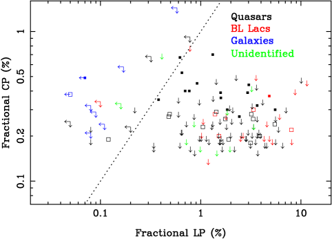
Figure 5: Plot of the absolute value of the fractional circular polarization versus fractional linear polarization for jet cores. Black points represent quasars, red points are BL Lac objects, blue points are galaxies, and unidentified objects appear in green. Solid squares are of $\geq 3\sigma$ significance, open squares are of $2$–$3\sigma$ significance, and arrows represent upper limits. The dashed line indicates $|m_{c}|=m_{l}$.

Figure 5 is a plot of absolute fractional core circular polarization, $|m_{c}|$, versus fractional core linear polarization, $m_{l}$. There is no clear relation between the two, and the obvious lack of correlation between linear and circular polarization is similar to the 5 GHz VLBA results of Homan et al. (2001), and the integrated 5 GHz measurements from the ATCA by Rayner et al. (2000). The persistence of no trend at higher frequency suggests that the complicating factors (lack of resolution/Faraday effects) are to some degree self-similar and scale-up with observing frequency.

Although there is no correlation between linear and circular polarization for jet cores, Figure 5 shows that for quasars and BL Lac objects, linear polarization almost always exceeds circular polarization. This does not seem to be the case for radio galaxies, which generally have weak linear polarization. Brunthaler et al. (2001) have noted that the nearby very low luminosity radio sources Sgr A* and M81* are circularly polarized but show no linear polarization. These authors have suggested that the $m_{c}/m_{l}$ ratio is distinctly different for low luminosity AGN ($m_{c}/m_{l}>>1$) and high luminosity AGN ($m_{c}/m_{l}<<1$). This relation was tested further by Bower et al. (2002), who failed to find additional LLAGN with circular polarization; however, if we consider the lowest redshift (and hence lowest luminosity) sources in our sample (which are admittedly quite different in character from the Sgr A* and M81*), we find that $m_{c}/m_{l}>>1$ for M87 (1228$+$126) and 3C 84 (0316$+$413), the only two radio galaxies for which we can do the comparison. Both M87 and 3C 84 are known to have strong external Faraday screens which can depolarize the linear polarization (Wardle, 1971; Zavala & Taylor, 2002), and in fact, all the radio galaxies in the MOJAVE sample have very low levels of core linear polarization, likely due to external depolarization. Higher redshift sources may have smaller $m_{c}/m_{l}$ ratios not because a different production mechanism for CP, but rather because either (1) they have less depolarization, and/or (2) we study them with less effective linear resolution and therefore polarization from more of the jet contributes to what we see as the ”core”. If (2) is the case, it also naturally explains the lack of correlation between $m_{c}$ and $m_{l}$ in Figure 5.

3.2 Circular Polarization of Jet Components

Table 3 lists circular polarization measurements for all strong jet components in our sample with peak Stokes-I $\geq 300$ mJy beam^-1. Of the 33 jet components that meet this criteria, we detect circular polarization in six (18%) of them at the $3\sigma$ level or higher significance. Five of these six detections are on the relatively nearby sources 3C 84 (0316$+$413) and 3C 273 (1226$+$023) which are discussed in more detail in section §3.3, and we note that 3C 84 is a special case as the distinction between the VLBI core and jet is not well defined and the circular polarization measured is unusually strong ($\gtrsim 1$%). For these reasons, we must be cautious about drawing conclusions about the circular polarization characteristics of jet components in general; however, it is clear that strong jet components can be circularly polarized, and the levels of circular polarization found in strong jet components are not clearly different from jet cores.

3.3 Discussion of Selected Sources

Here we discuss a few sources in detail, and we also compare our first epoch results with previous VLBA observations of circular polarization (HW99; Homan et al. (2001); Homan & Wardle (2003); Homan & Wardle (2004)) and from historical integrated measurements (1970s through early 1980s: Weiler & de Pater (1983), hereafter WdP83; Komesaroff et al. (1984), hereafter K84; Aller et al. (2003)). Because the latter are at lower frequency (typically 5 GHz and below) and are integrated measurements, we only compare to the historical circular polarization results in those cases where the source was repeatedly (three times or more) detected in circular polarization.

Because there is a large overlap of our sample with the sources observed at 5 GHz with the VLBA on 1996 December 15 by Homan et al. (2001), we list results from the latter study alongside our 15 GHz results in Table 5. We discuss some of the sources common to both of these studies in more detail below. The large number of limits from both programs makes the results in Table 5 difficult to interpret; however, it appears that CP of the core can vary with time and/or frequency.

0316$+$413 (3C 84):

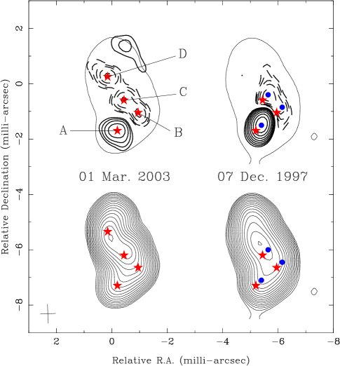
Figure 6: Circular polarization from the central 5 milli-arcseconds of 3C 84. The left-hand panels show our March 2003 observations, and the right-hand panels show the observations by Homan & Wardle (2004) from December of 1997. The images from both epochs have been convolved with an identical beam of 0.69$\times$0.55 mas$\times$mas, plotted as a cross in the lower left hand corner of the plot. The top images are circular polarization contours beginning at $\pm 2$ mJy beam^-1 and increasing in steps of $\times\sqrt{2}$. Dashed contours represent negative circular polarization. A single Stokes-$I$ contour shows the registration of the CP within this region. The bottom images are the Stokes-$I$ contours (beginning at $\pm 10$ mJy beam^-1 and increasing in steps of $\times\sqrt{2}$) from the same region. The four circularly polarized components from March 2003 are labelled with letters and their positions are marked with red stars. The three blue dots on the right hand image have the same relative positions as the red stars corresponding to components A–C, only they have been shifted by 0.2 milli-arcseconds to the west and by 0.2 milli-arcseconds to the north.

The left-hand panels of Figure 6 show the central 5 milli-arcseconds from our March 2003 MOJAVE observations of 3C 84. The image reveals four distinct spots of circular polarization within this central region of the source. Without a clear component to identify as the core, we have taken spot ”D” as the location of the VLBI core. Homan & Wardle (2004) found that even the locations corresponding to spots ”C” and ”B” were optically thick in December of 1997, so the precise definition of the jet core in this source is not clear. With only one frequency, we don’t know where the $\tau\sim 1$ surface is in 2003, so it is possible that all three spots of negative circular polarization: B, C, and D, may be part of an extended optically thick region; however, for the purposes of this paper, we have chosen to treat spots B and C as locations in the jet, along with spot A.

Both spots D and C are similarly circularly polarized at the $-0.4$% level; however, the strength of the circular polarization increases sharply in spot B to $-1.4$%. A little further out in the jet, but at quite a different position angle, spot A is more than $2$% circularly polarized with positive circular polarization. Homan & Wardle (2004) attribute this change in sign to the stark change in opacity they observe between spots B and A.

The circular polarization we observe is very similar to that seen by Homan & Wardle (2004) in observations more than 5 years earlier; however, spot D is entirely new and was not present in December of 1997. A version of the 15 GHz image from Homan & Wardle (2004) (convolved with a matching beam to our MOJAVE observations) appears in the right-hand panels of Figure 6. The 1997 image is registered with the 2003 image by matching contours on the northern-most end of the central region shown here. The red dots in the right-hand panels of Figure 6 have the same relative positions as the blue stars which mark the locations of spots A, B, and C in 2003, but they have been shifted by 0.2 milli-arcseconds to the North and by 0.2 milli-arcseconds to the West. It is clear that the relative positions of these circularly polarized spots has not changed significantly in 5$+$ years; however, they do appear to move outward together at a sub-luminal rate of roughly $0.06c$, almost directly South-East. This speed is, of course, dependent on our alignment of the images; however, it is similar to the speed found by Dhawan et al. (1998) at 43 GHz for two of the three component they studied within this region, although those two components were moving almost due South.

Homan & Wardle (2004) found spot A to have $m_{c}=+3.2\pm 0.1$% which is somewhat larger than the $m_{c}=+2.3\pm 0.3$% we measure five years later. The intensity at the location of spot A has faded by a factor of three, from 1.2 Jy beam^-1 to 0.4 Jy beam^-1, so presumably the region has become more optically thin. Multi-frequency observations are necessary to test if this is indeed the case, but if so, it is remarkable that this location has remained as strongly circularly polarized as it has. Homan & Wardle (2004) argued that Faraday conversion is responsible for the high levels of circular polarization detected here. Faraday conversion is strongly dependent on optical depth, and we would eventually expect a significant decline in circular polarization from this mechanism if this region of the jet is becoming increasingly optically thin (e.g., Wardle & Homan, 2003). It will be particularly interesting to follow the changes in spot A in future MOJAVE epochs.

Homan & Wardle (2004) found spots B and C to have $m_{c}=-0.7\pm 0.1$% and $m_{c}=-0.6\pm 0.1$% respectively at 15 GHz. Spot B has essentially doubled in circular polarization percentage in 5 years, and Spot C has not changed significantly within our uncertainties. Neither location has changed much in Stokes-$I$ intensity.

If the alignment between the epochs is correct, the lack of large changes in the circular polarization distribution between spots A, B, and C is surprising given their motion. The magnetic field order and particles responsible for producing this circular polarization must be in motion, however, this motion seems to have preserved the particular field characteristics responsible for the strong levels of circular polarization we observe.

0430$+$052 (3C 120):

We find a limit of $|m_{c}|<0.29$% in the core at 15 GHz in February of 2003. HW99 also found limits between 0.2 and 0.3% in the core at 15 GHz throughout 1996. Both signs of circular polarization (with a clear preference for positive CP) were detected intermittently in the historical integrated measurements (WdP83 and K84) at 8.9 GHz and below.

0528$+$134:

We find a limit of $|m_{c}|<0.18$% in the core at 15 GHz in February of 2003. HW99 detected multiple epochs of significant circular polarization at about the $m_{c}=-0.5$% level in the core at 15 GHz during 1996. During 1996, 0528$+$134 was undergoing a large outburst, peaking with an integrated core flux 4.6 times larger than observed in February 2003.

0607$-$157:

We find a limit of $|m_{c}|<0.21$% in the core at 15 GHz in March of 2003. Homan & Wardle (2003) measured only $m_{c}=-0.23\pm 0.12$% in the core at 15 GHz in January of 1998, but they simultaneously detected $m_{c}=-0.65\pm 0.07$% in the core at 8 GHz. Homan et al. (2001) detected circular polarization in core of $m_{c}=-0.18\pm 0.05$ % at 5 GHz thirteen months earlier in December of 1996. Aller et al. (2003) found strong circular polarization, $m_{c}=-0.23\pm 0.04$% at 4.8 GHz in integrated measurements with the UMRAO during the period 2001–2002.

0735$+$178:

We measure $m_{c}=-0.30\pm 0.11$ % in the core at 15 GHz in November of 2002. HW99 did not detect core circular polarization at 15 GHz at any epoch during 1996 with a typical limit of $|m_{c}|<0.4$%.

0851$+$202 (OJ287):

We measure $m_{c}=-0.20\pm 0.08$ % in the core at 15 GHz in October of 2002. HW99 did not detect core circular polarization at 15 GHz at any epoch during 1996, with a typical limit of $|m_{c}|<0.2$%. Homan et al. (2001) also found a limit of $|m_{c}|<0.10$% for the core circular polarization at 5 GHz in December of 1996. In older integrated measurements during the period 1978–1983, Aller et al. (2003) found strong CP at 4.8 and 8.0 GHz with $m_{c}=-0.37\pm 0.12$% and $m_{c}=-0.22\pm 0.03$% respectively.

0923$+$392 (4C 39.25):

We find a limit of $|m_{c}|<0.18$% in the core at 15 GHz in October of 2002. In older integrated measurements during the period 1978–1983, Aller et al. (2003) found strong CP at 4.8 GHz with $m_{c}=-0.21\pm 0.05$%.

1127$-$145:

We measure $m_{c}=-0.24\pm 0.10$ % in the core at 15 GHz in October of 2002. Negative circular polarization was repeatedly detected at 5 GHz and below in the historical integrated measurements cataloged by WdP83 and K84.

1222$+$216:

We find a limit of $|m_{c}|<0.35$% in the core at 15 GHz in February of 2003. HW99 also found limits between 0.1 and 0.2% in the core at 15 GHz throughout 1996.

1226$+$023 (3C 273):

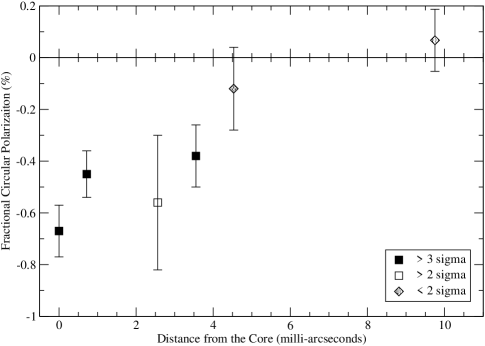
Figure 8: Plot of fractional circular polarization as a function of distance from the jet core for 3C 273. Note that the circular polarizaiton in 3C 273 predominantly has a negative sign and becomes weaker (going to smaller absolute values) at greater distances from the core. For the purposes of this plot, we have plotted all the values with their corresponding error bars, including those of $\lesssim 2\sigma$ significance.

Figure 7 shows the first 10 milli-arcseconds of the jet of 3C 273 at 15 GHz in October of 2002. The top panel is Stokes I, the middle panel is linear polarization, and the bottom panel is circular polarization. Positions where circular polarization measurements or limits were taken are marked and numbered on the Stokes I map. Figure 8 shows the fractional circular polarization at these locations as a function of distance from the jet core. The absolute fractional level of the circular polarization appears to decrease as distance from the core increases. This decrease could be tied to decreasing opacity along the jet or a decrease in poloidal magnetic field strength.

The core of 3C 273 was found by HW99 to have $m_{c}\simeq-0.5$% at three epochs during 1996. The circular polarization appeared with the emergence of a new jet component. The core was very opaque at this time, and HW99 showed that the appearance of the CP was tied to the flattening of the core’s spectral index due to the emergence of the new component. As cataloged in WdP83 and K84, 3C 273 was repeatedly detected in integrated measurements during the 1970s and early 80s at 8 GHz and below where it had a consistently negative sign of circular polarization.

1228$+$126 (M87):

Figure 9 shows our 15 GHz VLBA image of the jet of M87 in February of 2003. No linear polarization is detected, but strong circular polarization, $m_{c}=-0.49\pm 0.10$% is seen at the peak of the core.

M87 was studied at the VLA in April of 2000 by Bower et al. (2002), who found no significant circular polarization at 8 GHz, $m_{c}=0.01\pm 0.10$; however, they did find linear polarization at the $1.7$% level. These results are the opposite of our finding of strong circular polarization and no linear polarization. It is important to consider that their VLA results include contributions from the jet well beyond the region imaged by the VLBA, and the linear polarization they observe must come from beyond the depolarizing screen which covers most of the VLBA scale jet (Zavala & Taylor, 2002). The fractional circular polarization they measure may be diluted by emission beyond the VLBA scale, or the circular polarization may simply vary with frequency or time. Regardless, the differing linear polarizations observed between the VLBA and VLA scale images underscores our point from §3.1 that at least some of the lack of correlation between linear and circular polarization for jet cores could be due to the two quantities being produced in different regions of the unresolved jet core.

M87 has been detected intermittently in integrated circular polarization (with both signs) at 5 GHz and below in the historical observations cataloged by WdP83 and K84.

1253$-$055 (3C 279):

Figure 10 shows the first 5 milli-arcseconds of the jet of 3C 279 at 15 GHz in November of 2002. The top panel is Stokes I, the middle panel is linear polarization, and the bottom panel is circular polarization. Positions where circular polarization measurements or limits were taken are marked and numbered on the Stokes I map. We detect strong circular polarization of $m_{c}=+0.30\pm 0.08$% only on the jet core. The sign and magnitude of the circular polarization is consistent with five epochs of CP detections by HW99 at 15 GHz during 1996. At 5 GHz, Homan et al. (2001) did not detect circular polarization with a limit of $|m_{c}|<0.11$%. Historically, 3C 279 has repeatedly and consistently shown a positive sign for its circular polarization in integrated measurements at 8 GHz and below during the 1970s and early 80s (WdP83 and K84); however, Aller et al. (2003) found $m_{c}=-0.17\pm 0.01$% at 4.8 GHz with the UMRAO during 2001-2002. This change in sign at the lower frequency is particularly interesting as no change has yet occurred at 15 GHz.

1308$+$326:

We find a limit of $|m_{c}|<0.21$% in the core at 15 GHz in November of 2003. HW99 also found limits between 0.1 and 0.2% in the core at 15 GHz throughout 1996.

1510$-$089:

We measure $m_{c}=+0.20\pm 0.09$ % in the core at 15 GHz in November of 2002. HW99 did not detect circular polarization in the core at 15 GHz during 1996: three epochs had limits of 0.1 to 0.2%, and for two epochs they reported peak CP values of $+0.2\pm 0.2$ %. Homan et al. (2001) find a limit of $|m_{c}|<0.24$% in the core at 5 GHz in December of 1996.

1641$+$399 (3C 345):

We find a limit of $|m_{c}|<0.19$% in the core at 15 GHz in November of 2002. Homan & Wardle (2003) detected circular polarization in the core at 15 GHz, $m_{c}=-0.38\pm 012$%, in January of 1998. The same location was optically thick at 8 GHz where they did not detect any circular polarization in simultaneous measurements. 3C 345 was detected intermittently (and with both signs) at 8 GHz and below in the historical integrated measurement compiled by WdP83.

1730$-$130:

We find a limit of $|m_{c}|<0.17$% in the core at 15 GHz in October of 2002. The historical integrated measurements (WdP83 and K84) show several intermittent detections of positive circular polarization at 5 GHz and below.

1749$+$096:

We find a limit of $|m_{c}|<0.14$% in the core at 15 GHz in May of 2002. HW99 also found typical limits of 0.2% in the core at 15 GHz throughout 1996.

1928$+$738:

We measure $m_{c}=+0.19\pm 0.09$ % in the core at 15 GHz in June of 2002. HW99 also measured circular polarization in the core 15 GHz at the limit of their sensitivity. They found $m_{c}=+0.3\pm 0.1$ % in two epochs, $m_{c}=+0.2\pm 0.1$ % in one epoch, and limits of 0.1 and 0.2% in their other two epochs during 1996.

2134$+$004:

Figure 11 shows our observations of 2134$+$004 at 15 GHz in May of 2002. The top panel is Stokes I, the middle panel is linear polarization, and the bottom panel is circular polarization. Positions where circular polarization measurements or limits were taken are marked and numbered on the Stokes I map. We detect strong circular polarization of $m_{c}=+0.35\pm 0.12$% on the jet core, we measure a similar value at location number 1 of $m_{c}=+0.29\pm 0.12$%, and we find a limit on the CP at location 2 to be $|m_{c}|<0.34$%.

In recent integrated measurements from 2001–2002, Aller et al. (2003) found strong circular polarization at 4.8 GHz with $m_{c}=+0.62\pm 0.06$%. 2134$+$004 was also detected repeatedly in the historical integrated measurements at 5 GHz and below, always with positive circular polarization (WdP83 and K84).

2145$+$067:

We find a limit of $|m_{c}|<0.26$% in the core at 15 GHz in March of 2003. In recent integrated measurement from 2001–2002, Aller et al. (2003) measured $m_{c}=-0.50\pm 0.07$% at 4.8 GHz with the UMRAO. The historical integrated measurements (WdP83 and K84) show consistent, repeated detections of negative circular polarization at 5 GHz and below. Given this historical record of detection, it is interesting that the ’limit’ reported here came from measurements that had a significance of $1.98\sigma$, just barely less than the $2\sigma$ cutoff we had for defining measurements versus limits. If we allow $1.98\sigma$ as a measurement, then our fractional level for the core is $m_{c}=-0.17\pm 0.09$ %.

2200$+$420:

We find a limit of $|m_{c}|<0.21$% in the core at 15 GHz in June of 2002. WdP83 reported intermittent detections of both signs of circular polarization at frequencies below 5 GHz in the historical integrated measurements.

2230$+$114 (CTA102):

We find a limit of $|m_{c}|<0.19$% in the core at 15 GHz in October of 2002. Homan et al. (2001) measured $m_{c}=-0.09\pm 0.04$% in the core at 5 GHz in December of 1996. CTA102 was intermittently detected (with both signs of CP) in the historical integrated measurements (WdP83; K84) at 5 GHz and below.

2251$+$158 (3C 454.3):

Figure 12 shows the first 4 milli-arcseconds of the jet of 3C 454.3 at 15 GHz in March of 2003. Positions where circular polarization measurements or limits were taken are marked and numbered on the Stokes I map. The first jet component (position 1) appears slightly more strongly circularly polarized, $m_{c}=+0.38\pm 0.10$%, than the core, $m_{c}=+0.23\pm 0.10$%; however, an alternative calibration assuming no circular polarization for calibrating the phases (see §2.2) spreads the circular polarization between the core and component 1 more evenly with both having $m_{c}\simeq 0.3$%.

Homan et al. (2001) measured $m_{c}=+0.08\pm 0.04$% in the core of 3C 454.3 at 5 GHz in December of 1996, and the source was repeatedly detected with positive circular polarization at 8 GHz and below in the integrated historical measurements compiled by WdP83 and K84.

2345$-$167:

We detect $m_{c}=+0.40\pm 0.11$% in the core at 15 GHz in October of 2002. Homan et al. (2001) found a limit of $|m_{c}|<0.11$% in the core at 5 GHz in December of 1996. WdP83 and K84 reported intermittent detections (but always with positive sign) of circular polarization in integrated measurements at frequencies of 5 GHz and below.

4 Conclusions

In this paper, we report first-epoch circular polarization results for each of the 133 AGN in the MOJAVE program to monitor the VLBA structure and polarization of a flux limited sample of AGN jets at 15 GHz. We found strong circular polarization ($\geq 0.3$%) in approximately 15% of our sample. The circular polarization we detected was usually associated with jet cores, typically in the range of $0.3-0.5$% of the local Stokes-$I$. Our ability to detect circular polarization on jet components was limited by their relatively weak flux density; however, we did find a few strong jet components to be circularly polarized.

We found no significant correlations between fractional circular polarization of jet cores and optical source type, redshift, EGRET detections, linear polarization, or a number of other pc-scale jet properties listed in Table 4. While there was no clear relation between linear and circular polarization of jet cores, quasars and BL Lac objects consistently had more linear than circular polarization, and the two galaxies with detected circular polarization had much more circular than linear polarization. We suggested that higher redshift sources may have smaller $m_{c}/m_{l}$ ratios, not because they produce circular polarization differently from low redshift sources, but rather because either (1) they have less depolarization, and/or (2) we study them with less effective linear resolution and therefore polarization from more of the jet contributes to what we see as the “core”.

The lack of clear correlations between circular polarization and other source properties is intriguing, particularly given that some sources, 3C 273 and 3C 279 in particular, show consistently high levels of circular polarization over years and decades of observation, even though they are both known to be highly variable with regular ($\sim$ annual) ejections of new jet components. It seems highly unlikely that these sources would be circularly polarized in a very similar fashion from epoch to epoch due only to stochastic factors (such as a chance favorable magnetic field configuration). It may be that we simply detect too few sources in circular polarization to find subtle trends between circular polarization and other source properties, or perhaps, even with the VLBA we are not resolving the core region well enough to see where the circular polarization is being generated.

In addition to looking for overall trends in the circular polarization of our sample, we also examined the structure of a few sources in detail. 3C 84 was particularly interesting, showing the strongest circular polarization in our sample, up to $2$% in one location. Our image revealed essentially the same structure as Homan & Wardle (2004) found in data taken five years earlier; however, a new circularly polarized spot appeared in our data, and the older spots of circular polarization, while maintaining the same relative positions, appear to have moved outward in the jet at a rate of approximately 0.06$c$. 3C 273 also showed multiple locations of circular polarization in its jet, and we were able to plot circular polarization measurements for several strong jet components. This plot revealed that, in 3C 273, fractional circular polarization gets weaker at greater distances from the jet core. Multi-frequency observations will be necessary for both sources so we can use opacity measurements to help understand the trends of circular polarization with jet position.

Table 1: Circular Polarization at Stokes $I$ Peak.

IAU			Opt.		$I_{peak}$	$m_{l}$	$V_{peak}$	$m_{c}$
Name	Alias	z	Class	Epoch	(Jy beam-1)	(%)	(mJy beam-1)	(%)	$\sigma$
(1)	(2)	(3)	(4)	(5)	(6)	(7)	(8)	(9)	(10)
$0003-066$	NRAO 005	$0.347$	B	2003 Feb 06	$1.83$	$4.30$	$+1.55\pm 1.82$	$<0.20$	$\cdots$
$0007+106$	III Zw 2	$0.0893$	G	2004 Feb 11	$1.35$	$<0.08$	$-2.74\pm 1.54$	$<0.32$	$\cdots$
$0016+731$	$\cdots$	$1.781$	Q	2003 Aug 28	$0.99$	$0.97$	$+1.02\pm 1.73$	$<0.35$	$\cdots$
$0048-097$	$\cdots$	$\cdots$	B	2003 Aug 28	$0.70$	$3.57$	$-0.74\pm 1.78$	$<0.51$	$\cdots$
$0059+581$	$\cdots$	$\cdots$	U	2002 Nov 23	$3.16$	$1.96$	$+1.22\pm 2.68$	$<0.17$	$\cdots$
$0106+013$	$\cdots$	$2.107$	Q	2003 Mar 29	$2.13$	$1.54$	$+1.27\pm 2.07$	$<0.19$	$\cdots$
$0109+224$	$\cdots$	$\cdots$	B	2002 Jun 15	$0.93$	$4.58$	$-0.82\pm 1.14$	$<0.25$	$\cdots$
$0119+115$	$\cdots$	$0.57$	Q	2003 Mar 01	$0.88$	$5.58$	$-0.01\pm 1.18$	$<0.27$	$\cdots$
$0133+476$	DA 55	$0.859$	Q	2002 Jun 15	$4.20$	$3.14$	$-7.79\pm 3.69$	$-0.18\pm 0.09$	2.1
$0202+149$	4C $+$15.05	$0.405$	Q	2002 Oct 09	$1.23$	$0.08$	$+0.23\pm 1.39$	$<0.23$	$\cdots$
$0202+319$	$\cdots$	$1.466$	Q	2003 Mar 29	$2.10$	$1.57$	$+2.03\pm 2.00$	$<0.19$	$\cdots$
$0212+735$	$\cdots$	$2.367$	Q	2003 May 09	$1.25$	$10.90$	$+2.46\pm 1.35$	$<0.31$	$\cdots$
$0215+015$	$\cdots$	$1.715$	B	2002 May 31	$0.75$	$1.39$	$+2.10\pm 0.89$	$+0.28\pm 0.12$	2.4
$0224+671$	4C $+$67.05	$\cdots$	U	2002 Nov 23	$0.68$	$0.86$	$0.00\pm 0.86$	$<0.25$	$\cdots$
$0234+285$	CTD 20	$1.213$	Q	2002 Nov 23	$3.42$	$0.79$	$+2.82\pm 2.88$	$<0.17$	$\cdots$
$0235+164$	$\cdots$	$0.94$	B	2003 Mar 01	$1.45$	$4.85$	$-1.45\pm 1.45$	$<0.20$	$\cdots$
$0238-084$	NGC 1052	$0.0049$	G	2002 Oct 09	$0.34$	$<0.58$	$+0.83\pm 2.43$	$<1.44$	$\cdots$
$0300+470$	4C $+$47.08	$\cdots$	B	2002 Nov 23	$1.04$	$1.02$	$+0.12\pm 1.09$	$<0.21$	$\cdots$
$0316+413$	3C 84	$0.01756$	G	2003 Mar 01	$2.65$	$<0.04$	$-4.87\pm 3.67$	$<0.32$	$\cdots$
$0333+321$	NRAO 140	$1.263$	Q	2003 Mar 29	$1.73$	$0.49$	$-4.88\pm 1.82$	$-0.28\pm 0.10$	2.7
$0336-019$	CTA 26	$0.852$	Q	2003 Feb 06	$2.72$	$4.37$	$+1.47\pm 2.47$	$<0.18$	$\cdots$
$0403-132$	$\cdots$	$0.571$	Q	2002 May 31	$1.32$	$0.62$	$+0.21\pm 1.21$	$<0.18$	$\cdots$
$0415+379$	3C 111	$0.0491$	G	2002 Oct 09	$1.17$	$<0.08$	$-0.22\pm 1.21$	$<0.21$	$\cdots$
$0420-014$	$\cdots$	$0.915$	Q	2003 Mar 01	$9.46$	$0.87$	$+1.58\pm 7.62$	$<0.16$	$\cdots$
$0422+004$	$\cdots$	$\cdots$	B	2002 Jun 15	$1.64$	$8.11$	$+1.18\pm 1.58$	$<0.19$	$\cdots$
$0430+052$	3C 120	$0.033$	G	2003 Feb 06	$1.04$	$<0.09$	$+1.92\pm 1.10$	$<0.29$	$\cdots$
$0446+112$	$\cdots$	$1.207$	Q	2002 May 31	$2.11$	$1.14$	$-2.30\pm 1.85$	$<0.20$	$\cdots$
$0458-020$	$\cdots$	$2.286$	Q	2003 Mar 01	$1.04$	$1.29$	$-0.03\pm 1.23$	$<0.24$	$\cdots$
$0528+134$	$\cdots$	$2.07$	Q	2003 Feb 06	$2.64$	$4.55$	$+0.95\pm 2.37$	$<0.18$	$\cdots$
$0529+075$	$\cdots$	$\cdots$	U	2002 May 31	$0.69$	$0.41$	$-2.17\pm 2.46$	$<0.71$	$\cdots$
$0529+483$	$\cdots$	$1.162$	Q	2002 Oct 09	$0.90$	$1.99$	$-0.22\pm 0.95$	$<0.21$	$\cdots$
$0552+398$	DA 193	$2.363$	Q	2003 Mar 29	$2.39$	$1.60$	$-2.48\pm 2.23$	$<0.20$	$\cdots$
$0605-085$	$\cdots$	$0.872$	Q	2003 Feb 06	$1.00$	$2.54$	$-0.92\pm 1.32$	$<0.26$	$\cdots$
$0607-157$	$\cdots$	$0.324$	Q	2003 Mar 01	$4.04$	$3.65$	$+5.09\pm 3.42$	$<0.21$	$\cdots$
$0642+449$	OH 471	$3.408$	Q	2003 Mar 29	$3.46$	$2.94$	$+13.57\pm 2.96$	$+0.39\pm 0.09$	4.6
$0648-165$	$\cdots$	$\cdots$	U	2002 Nov 23	$2.31$	$0.99$	$-1.93\pm 1.97$	$<0.17$	$\cdots$
$0716+714$	$\cdots$	$\cdots$	B	2003 Aug 28	$2.51$	$4.84$	$+9.34\pm 2.82$	$+0.37\pm 0.11$	3.3
$0727-115$	$\cdots$	$1.591$	Q	2003 Mar 01	$4.09$	$3.14$	$-3.44\pm 3.68$	$<0.18$	$\cdots$
$0730+504$	$\cdots$	$0.72$	Q	2002 Jun 15	$0.72$	$0.65$	$-3.78\pm 1.20$	$-0.53\pm 0.17$	3.2
$0735+178$	$\cdots$	$\cdots$	B	2002 Nov 23	$0.85$	$3.36$	$-2.57\pm 0.92$	$-0.30\pm 0.11$	2.8
$0736+017$	$\cdots$	$0.191$	Q	2003 Mar 01	$1.49$	$0.92$	$+6.66\pm 1.41$	$+0.45\pm 0.09$	4.7
$0738+313$	OI 363	$0.63$	Q	2003 Feb 06	$0.51$	$0.42$	$-1.79\pm 1.65$	$<0.68$	$\cdots$
$0742+103$	$\cdots$	$\cdots$	U	2004 Feb 11	$0.59$	$<0.16$	$-0.31\pm 0.96$	$<0.33$	$\cdots$
$0748+126$	$\cdots$	$0.889$	Q	2003 Feb 06	$1.79$	$3.37$	$+2.69\pm 1.66$	$<0.24$	$\cdots$
$0754+100$	$\cdots$	$0.266$	B	2002 Nov 23	$1.38$	$6.12$	$-2.46\pm 1.36$	$<0.28$	$\cdots$
$0804+499$	$\cdots$	$1.432$	Q	2004 Feb 11	$0.61$	$0.60$	$-0.27\pm 1.11$	$<0.36$	$\cdots$
$0805-077$	$\cdots$	$1.837$	Q	2002 Jun 15	$1.28$	$0.64$	$+0.71\pm 1.41$	$<0.22$	$\cdots$
$0808+019$	$\cdots$	$\cdots$	B	2004 Feb 11	$0.46$	$8.75$	$+0.43\pm 0.92$	$<0.41$	$\cdots$
$0814+425$	$\cdots$	$\cdots$	B	2004 Feb 11	$0.67$	$1.79$	$+0.47\pm 0.96$	$<0.28$	$\cdots$
$0823+033$	$\cdots$	$0.506$	B	2003 Jun 15	$0.97$	$1.06$	$+0.20\pm 1.23$	$<0.26$	$\cdots$
$0827+243$	$\cdots$	$0.941$	Q	2002 May 31	$1.77$	$0.08$	$-1.37\pm 1.64$	$<0.19$	$\cdots$
$0829+046$	$\cdots$	$0.18$	B	2003 Aug 28	$0.43$	$0.78$	$+0.60\pm 1.69$	$<0.80$	$\cdots$
$0836+710$	$\cdots$	$2.218$	Q	2003 Mar 29	$1.19$	$0.70$	$+4.72\pm 1.20$	$+0.40\pm 0.10$	3.9
$0851+202$	OJ 287	$0.306$	B	2002 Oct 09	$3.48$	$1.52$	$-6.90\pm 2.88$	$-0.20\pm 0.08$	2.4
$0906+015$	4C $+$01.24	$1.018$	Q	2003 Mar 29	$1.91$	$5.59$	$-0.23\pm 1.80$	$<0.19$	$\cdots$
$0917+624$	$\cdots$	$1.446$	Q	2002 Jun 15	$0.57$	$3.61$	$-1.01\pm 1.27$	$<0.44$	$\cdots$
$0923+392$	4C $+$39.25	$0.698$	Q	2002 Oct 09	$4.33$	$2.05$	$+4.09\pm 3.76$	$<0.18$	$\cdots$
$0945+408$	$\cdots$	$1.252$	Q	2002 Oct 09	$1.00$	$1.84$	$+3.03\pm 1.02$	$+0.30\pm 0.10$	3.0
$0955+476$	$\cdots$	$1.873$	Q	2002 Jun 15	$1.56$	$0.86$	$-2.73\pm 1.60$	$<0.28$	$\cdots$
$1036+054$	$\cdots$	$\cdots$	U	2002 May 31	$2.55$	$1.45$	$+1.86\pm 1.99$	$<0.16$	$\cdots$
$1038+064$	$\cdots$	$1.265$	Q	2002 May 31	$1.03$	$0.60$	$-1.97\pm 1.06$	$<0.29$	$\cdots$
$1045-188$	$\cdots$	$0.595$	Q	2002 Jun 15	$1.11$	$3.26$	$+1.99\pm 1.64$	$<0.33$	$\cdots$
$1055+018$	4C $+$01.28	$0.888$	Q	2003 Feb 06	$3.15$	$3.66$	$+10.10\pm 2.82$	$+0.32\pm 0.09$	3.6
$1124-186$	$\cdots$	$1.048$	Q	2003 Mar 01	$1.30$	$1.94$	$+2.67\pm 1.49$	$<0.32$	$\cdots$
$1127-145$	$\cdots$	$1.187$	Q	2002 Oct 09	$1.07$	$5.49$	$-2.60\pm 1.12$	$-0.24\pm 0.10$	2.3
$1150+812$	$\cdots$	$1.25$	Q	2002 Jun 15	$0.98$	$0.72$	$+1.23\pm 1.20$	$<0.25$	$\cdots$
$1156+295$	4C $+$29.45	$0.729$	Q	2002 Nov 23	$1.86$	$2.43$	$-5.02\pm 1.70$	$-0.27\pm 0.09$	3.0
$1213-172$	$\cdots$	$\cdots$	U	2002 Jun 15	$1.11$	$4.18$	$+0.61\pm 1.39$	$<0.25$	$\cdots$
$1219+044$	$\cdots$	$0.965$	Q	2002 Jun 15	$0.91$	$0.22$	$+1.72\pm 1.12$	$<0.31$	$\cdots$
$1222+216$	$\cdots$	$0.435$	Q	2002 May 31	$0.56$	$4.15$	$-1.13\pm 0.81$	$<0.35$	$\cdots$
$1226+023$	3C 273	$0.158$	Q	2002 Oct 09	$8.99$	$3.74$	$-40.28\pm 8.07$	$-0.45\pm 0.09$	5.0
$1228+126$	M87	$0.0044$	G	2003 Feb 06	$1.28$	$<0.07$	$-6.32\pm 1.34$	$-0.49\pm 0.10$	4.7
$1253-055$	3C 279	$0.538$	Q	2002 Nov 23	$10.31$	$5.53$	$+30.52\pm 8.67$	$+0.30\pm 0.08$	3.5
$1308+326$	$\cdots$	$0.997$	Q	2002 Nov 23	$2.00$	$3.26$	$+2.30\pm 1.99$	$<0.21$	$\cdots$
$1324+224$	$\cdots$	$1.4$	Q	2002 Oct 09	$0.55$	$1.33$	$+1.10\pm 0.96$	$<0.37$	$\cdots$
$1334-127$	$\cdots$	$0.539$	Q	2003 Mar 01	$4.31$	$1.43$	$+12.71\pm 4.47$	$+0.29\pm 0.10$	2.8
$1413+135$	$\cdots$	$0.247$	B	2002 Nov 23	$0.88$	$<0.10$	$-1.89\pm 1.10$	$<0.34$	$\cdots$
$1417+385$	$\cdots$	$1.832$	Q	2002 Jun 15	$0.84$	$2.04$	$-0.51\pm 1.08$	$<0.26$	$\cdots$
$1458+718$	3C 309.1	$0.904$	Q	2003 Aug 28	$0.58$	$1.43$	$+0.77\pm 1.39$	$<0.48$	$\cdots$
$1502+106$	4C $+$10.39	$1.833$	Q	2003 Mar 29	$1.45$	$1.01$	$-1.54\pm 1.40$	$<0.20$	$\cdots$
$1504-166$	$\cdots$	$0.876$	Q	2003 Feb 06	$0.93$	$1.76$	$+2.43\pm 1.07$	$+0.26\pm 0.12$	2.3
$1510-089$	$\cdots$	$0.36$	Q	2002 Nov 23	$2.73$	$3.88$	$+5.51\pm 2.40$	$+0.20\pm 0.09$	2.3
$1538+149$	4C $+$14.60	$0.605$	B	2004 Feb 11	$0.97$	$11.50$	$-2.80\pm 1.82$	$<0.47$	$\cdots$
$1546+027$	$\cdots$	$0.412$	Q	2003 Mar 29	$1.42$	$1.81$	$-0.88\pm 1.66$	$<0.24$	$\cdots$
$1548+056$	4C $+$05.64	$1.422$	Q	2003 Mar 01	$1.66$	$3.24$	$-0.38\pm 1.68$	$<0.20$	$\cdots$
$1606+106$	4C $+$10.45	$1.226$	Q	2002 Nov 23	$1.48$	$2.55$	$-0.06\pm 1.59$	$<0.21$	$\cdots$
$1611+343$	DA 406	$1.401$	Q	2003 Feb 06	$2.72$	$2.97$	$-3.44\pm 2.45$	$<0.22$	$\cdots$
$1633+382$	4C $+$38.41	$1.807$	Q	2003 Mar 29	$3.48$	$1.58$	$-13.59\pm 3.02$	$-0.39\pm 0.09$	4.5
$1637+574$	$\cdots$	$0.751$	Q	2002 May 31	$1.65$	$1.64$	$+0.67\pm 1.39$	$<0.17$	$\cdots$
$1638+398$	NRAO 512	$1.666$	Q	2003 Mar 01	$0.68$	$7.10$	$-1.15\pm 0.97$	$<0.31$	$\cdots$
$1641+399$	3C 345	$0.594$	Q	2002 Nov 23	$2.95$	$3.53$	$-0.04\pm 2.83$	$<0.19$	$\cdots$
$1655+077$	$\cdots$	$0.621$	Q	2002 Oct 09	$0.86$	$3.20$	$+2.40\pm 0.93$	$+0.28\pm 0.11$	2.6
$1726+455$	$\cdots$	$0.714$	Q	2002 May 31	$2.07$	$3.71$	$-0.64\pm 1.65$	$<0.16$	$\cdots$
$1730-130$	NRAO 530	$0.902$	Q	2002 Oct 09	$4.75$	$0.34$	$+0.37\pm 3.92$	$<0.17$	$\cdots$
$1739+522$	4C $+$51.37	$1.379$	Q	2003 Mar 29	$1.30$	$2.86$	$-0.59\pm 1.32$	$<0.20$	$\cdots$
$1741-038$	$\cdots$	$1.057$	Q	2003 Mar 01	$5.96$	$0.65$	$-7.59\pm 5.34$	$<0.22$	$\cdots$
$1749+096$	4C $+$09.57	$0.32$	B	2002 May 31	$3.13$	$1.19$	$+1.10\pm 2.28$	$<0.14$	$\cdots$
$1751+288$	$\cdots$	$\cdots$	U	2002 Jun 15	$1.84$	$0.72$	$+1.62\pm 1.75$	$<0.19$	$\cdots$
$1758+388$	$\cdots$	$2.092$	Q	2003 May 09	$1.26$	$1.21$	$-1.30\pm 1.07$	$<0.19$	$\cdots$
$1800+440$	$\cdots$	$0.663$	Q	2003 Mar 29	$1.10$	$1.32$	$+7.71\pm 1.21$	$+0.70\pm 0.11$	6.3
$1803+784$	$\cdots$	$0.68$	B	2003 Feb 06	$1.33$	$2.50$	$+1.27\pm 1.35$	$<0.20$	$\cdots$
$1823+568$	4C $+$56.27	$0.663$	B	2003 May 09	$1.32$	$8.05$	$+2.96\pm 1.17$	$+0.22\pm 0.09$	2.5
$1828+487$	3C 380	$0.692$	Q	2003 Mar 29	$1.28$	$2.26$	$-0.02\pm 3.27$	$<0.51$	$\cdots$
$1849+670$	$\cdots$	$0.657$	Q	2003 Jun 15	$1.59$	$3.34$	$-4.10\pm 1.84$	$-0.26\pm 0.12$	2.2
$1928+738$	4C $+$73.18	$0.303$	Q	2002 Jun 15	$2.47$	$0.12$	$+4.78\pm 2.23$	$+0.19\pm 0.09$	2.1
$1936-155$	$\cdots$	$1.657$	Q	2002 May 31	$0.73$	$1.59$	$+2.65\pm 0.88$	$+0.36\pm 0.12$	3.0
$1957+405$	Cygnus A	$0.056$	G	2002 Nov 23	$0.64$	$<0.17$	$+1.21\pm 1.85$	$<0.58$	$\cdots$
$1958-179$	$\cdots$	$0.652$	Q	2002 May 31	$0.95$	$0.48$	$+2.56\pm 1.03$	$+0.27\pm 0.11$	2.5
$2005+403$	$\cdots$	$1.736$	Q	2003 Mar 01	$1.56$	$3.94$	$+0.94\pm 1.65$	$<0.21$	$\cdots$
$2008-159$	$\cdots$	$1.18$	Q	2003 Jun 15	$1.96$	$<0.05$	$+2.80\pm 2.06$	$<0.25$	$\cdots$
$2021+317$	4C $+$31.56	$\cdots$	U	2003 Feb 06	$0.39$	$3.22$	$-0.04\pm 0.85$	$<0.43$	$\cdots$
$2021+614$	$\cdots$	$0.227$	G	2003 Mar 01	$0.99$	$<0.11$	$+0.18\pm 1.18$	$<0.24$	$\cdots$
$2037+511$	3C 418	$1.687$	Q	2002 Oct 09	$1.62$	$0.97$	$+1.63\pm 1.54$	$<0.20$	$\cdots$
$2121+053$	$\cdots$	$1.941$	Q	2003 Mar 29	$2.13$	$6.56$	$-1.60\pm 1.92$	$<0.18$	$\cdots$
$2128-123$	$\cdots$	$0.501$	Q	2003 May 09	$1.78$	$1.72$	$+3.86\pm 1.63$	$+0.22\pm 0.09$	2.4
$2131-021$	4C $-$02.81	$1.285$	B	2003 May 09	$1.14$	$5.20$	$+1.11\pm 1.10$	$<0.19$	$\cdots$
$2134+004$	$\cdots$	$1.932$	Q	2002 May 31	$1.62$	$0.38$	$+5.63\pm 1.89$	$+0.35\pm 0.12$	3.0
$2136+141$	OX 161	$2.427$	Q	2002 Nov 23	$2.15$	$3.02$	$+9.45\pm 2.23$	$+0.44\pm 0.10$	4.2
$2145+067$	4C $+$06.69	$0.999$	Q	2003 Mar 01	$5.88$	$1.56$	$-10.11\pm 5.12$	$<0.26$	$\cdots$
$2155-152$	$\cdots$	$0.672$	Q	2003 Mar 29	$1.27$	$3.66$	$-1.97\pm 1.43$	$<0.27$	$\cdots$
$2200+420$	BL Lac	$0.069$	B	2002 Jun 15	$1.25$	$2.65$	$-0.15\pm 1.30$	$<0.21$	$\cdots$
$2201+171$	$\cdots$	$1.076$	Q	2003 Jun 15	$1.83$	$1.90$	$+3.42\pm 1.70$	$+0.19\pm 0.09$	2.0
$2201+315$	4C $+$31.63	$0.298$	Q	2002 Nov 23	$2.23$	$2.82$	$+0.74\pm 2.18$	$<0.20$	$\cdots$
$2209+236$	$\cdots$	$1.125$	Q	2003 Mar 01	$0.62$	$10.08$	$-1.98\pm 1.06$	$<0.49$	$\cdots$
$2216-038$	$\cdots$	$0.901$	Q	2002 May 31	$1.95$	$2.17$	$+0.27\pm 1.64$	$<0.17$	$\cdots$
$2223-052$	3C 446	$1.404$	Q	2002 Oct 09	$3.72$	$3.81$	$+4.45\pm 3.67$	$<0.22$	$\cdots$
$2227-088$	PHL 5225	$1.562$	Q	2003 Mar 29	$1.88$	$0.34$	$+0.67\pm 1.71$	$<0.18$	$\cdots$
$2230+114$	CTA 102	$1.037$	Q	2002 Oct 09	$2.32$	$1.67$	$+0.12\pm 2.22$	$<0.19$	$\cdots$
$2243-123$	$\cdots$	$0.63$	Q	2002 Oct 09	$1.03$	$1.32$	$+0.97\pm 1.27$	$<0.25$	$\cdots$
$2251+158$	3C 454.3	$0.859$	Q	2003 Mar 29	$3.25$	$1.05$	$+7.35\pm 3.32$	$+0.23\pm 0.10$	2.2
$2331+073$	$\cdots$	$\cdots$	U	2002 Jun 15	$0.96$	$3.38$	$+1.26\pm 1.06$	$<0.24$	$\cdots$
$2345-167$	$\cdots$	$0.576$	Q	2002 Oct 09	$1.39$	$0.77$	$+5.55\pm 1.48$	$+0.40\pm 0.11$	3.8
$2351+456$	4C $+$45.51	$1.986$	Q	2002 May 31	$1.39$	$2.09$	$+2.83\pm 1.45$	$<0.31$	$\cdots$

Note. — Columns are as follows: (1) IAU Name (B1950); (2) Other Name; (3) Redshift (see Lister & Homan, 2005, for references); (4) Optical classification where Q = quasar, B = BL Lac object, G = active galaxy, and U = unidentified; (5) Epoch of first observation in MOJAVE program; (6) Stokes $I$ at the map peak; (7) Fractional linear polarization of the Stokes $I$ peak; (8) Maximum circular polarization measured within two pixels of the Stokes $I$ peak; (9) Fractional circular polarization corresponding to Stokes-$V$ in column (8); (10) Significance of the circular polarization measurement: $|m_{c}|/\Delta m_{c}$.

Table 2: Circular Polarization on Off-Peak Jet Cores.

IAU	$R$	$\theta$	$I_{core}$	$m_{l}$	$V_{core}$	$m_{c}$
Name	(marcsec)	(deg.)	(Jy beam-1)	(%)	(mJy beam-1)	(%)	$\sigma$
(1)	(2)	(3)	(4)	(5)	(6)	(7)	(8)
$0212+735$	$0.67$	$-63.4$	$0.79$	$5.97$	$+0.21\pm 0.90$	$<0.23$	$\cdots$
$0316+413$	$0.28$	$45.0$	$2.26$	$<0.05$	$-8.61\pm 3.15$	$-0.38\pm 0.14$	2.7
$0738+313$	$3.71$	$-4.6$	$0.33$	$<0.32$	$+0.37\pm 1.12$	$<0.68$	$\cdots$
$0923+392$	$2.75$	$-79.5$	$0.19$	$<0.78$	$-0.95\pm 0.81$	$<0.92$	$\cdots$
$1213-172$	$0.50$	$-53.1$	$0.53$	$1.84$	$+0.86\pm 0.71$	$<0.30$	$\cdots$
$1226+023$	$0.72$	$56.3$	$2.78$	$0.62$	$-18.77\pm 2.71$	$-0.67\pm 0.10$	6.9
$1548+056$	$0.63$	$161.6$	$1.25$	$1.51$	$-0.20\pm 1.29$	$<0.21$	$\cdots$
$2128-123$	$1.12$	$26.6$	$0.43$	$<0.20$	$-0.20\pm 0.51$	$<0.23$	$\cdots$

Note. — Columns are as follows: (1) IAU Name (B1950); (2) Radial position of the core relative to the map peak; (3) Structural position angle of the core relative to the map peak; (4) Peak Stokes $I$ at the core position; (5) Fractional linear polarization at the core position; (6) Maximum circular polarization measured within two pixels of the core; (7) Fractional circular polarization corresponding to Stokes $V$ in column(6); (8) Significance of the circular polarization measurement: $|m_{c}|/\Delta m_{c}$.

Table 3: Circular Polarization on Strong Jet Components.

IAU	$R$	$\theta$	$I_{comp}$	$m_{l}$	$V_{comp}$	$m_{c}$
Name	(marcsec)	(deg.)	(Jy beam-1)	(%)	(mJy beam-1)	(%)	$\sigma$
(1)	(2)	(3)	(4)	(5)	(6)	(7)	(8)
$0212+735$	$0.67$	$116.6$	$1.25$	$10.90$	$+2.46\pm 1.35$	$<0.31$	$\cdots$
$0224+671$	$0.41$	$14.0$	$0.60$	$1.17$	$+0.12\pm 0.78$	$<0.26$	$\cdots$
$0316+413$	$1.00$	$-143.1$	$2.00$	$<0.06$	$-8.43\pm 2.82$	$-0.42\pm 0.14$	3.0
$0316+413$	$1.77$	$-137.3$	$0.65$	$<0.17$	$-8.93\pm 1.13$	$-1.37\pm 0.17$	7.9
$0316+413$	$1.94$	$-168.1$	$0.34$	$<0.34$	$+7.56\pm 0.84$	$+2.25\pm 0.25$	9.0
$0552+398$	$0.85$	$-69.4$	$0.33$	$<0.37$	$-0.34\pm 0.48$	$<0.29$	$\cdots$
$0738+313$	$3.71$	$175.4$	$0.51$	$0.42$	$-1.79\pm 1.65$	$<0.68$	$\cdots$
$0754+100$	$1.22$	$9.5$	$0.31$	$4.03$	$-0.13\pm 0.39$	$<0.25$	$\cdots$
$0851+202$	$1.25$	$-118.6$	$0.37$	$7.73$	$+0.61\pm 0.52$	$<0.30$	$\cdots$
$0923+392$	$2.75$	$100.5$	$4.33$	$2.05$	$+4.09\pm 3.76$	$<0.18$	$\cdots$
$0945+408$	$0.94$	$122.0$	$0.33$	$2.77$	$+0.75\pm 0.44$	$<0.36$	$\cdots$
$1038+064$	$0.71$	$171.9$	$0.49$	$1.29$	$-0.81\pm 0.56$	$<0.28$	$\cdots$
$1127-145$	$0.51$	$101.3$	$0.57$	$7.30$	$-0.35\pm 0.63$	$<0.22$	$\cdots$
$1213-172$	$0.50$	$126.9$	$1.11$	$4.18$	$+0.61\pm 1.39$	$<0.25$	$\cdots$
$1226+023$	$0.72$	$-123.7$	$8.99$	$3.74$	$-40.28\pm 8.07$	$-0.45\pm 0.09$	5.0
$1226+023$	$2.56$	$-120.6$	$0.46$	$6.33$	$-2.59\pm 1.18$	$-0.56\pm 0.26$	2.2
$1226+023$	$3.55$	$-130.4$	$1.28$	$7.08$	$-4.88\pm 1.59$	$-0.38\pm 0.12$	3.1
$1226+023$	$4.53$	$-131.4$	$0.82$	$4.20$	$-1.00\pm 1.33$	$<0.32$	$\cdots$
$1226+023$	$9.75$	$-115.5$	$1.49$	$9.97$	$+0.10\pm 1.73$	$<0.23$	$\cdots$
$1253-055$	$1.36$	$-126.0$	$1.04$	$24.91$	$-0.10\pm 1.65$	$<0.32$	$\cdots$
$1253-055$	$2.83$	$-122.0$	$0.52$	$38.68$	$+0.38\pm 1.47$	$<0.56$	$\cdots$
$1253-055$	$4.99$	$-122.7$	$0.54$	$10.93$	$-1.40\pm 1.47$	$<0.55$	$\cdots$
$1548+056$	$0.63$	$-18.4$	$1.66$	$3.24$	$-0.38\pm 1.68$	$<0.20$	$\cdots$
$1641+399$	$1.10$	$-90.0$	$1.53$	$4.14$	$+1.05\pm 1.66$	$<0.22$	$\cdots$
$1641+399$	$2.31$	$-95.0$	$0.33$	$3.43$	$-0.77\pm 0.96$	$<0.58$	$\cdots$
$1928+738$	$0.98$	$156.0$	$0.52$	$1.58$	$+1.09\pm 0.61$	$<0.33$	$\cdots$
$2128-123$	$1.12$	$-153.4$	$1.78$	$1.72$	$+3.86\pm 1.63$	$+0.22\pm 0.09$	2.4
$2131-021$	$0.76$	$113.2$	$0.61$	$1.92$	$+0.46\pm 0.63$	$<0.21$	$\cdots$
$2134+004$	$0.80$	$-90.0$	$0.77$	$8.54$	$+2.21\pm 0.94$	$+0.29\pm 0.12$	2.4
$2134+004$	$2.02$	$-98.5$	$1.33$	$4.99$	$+2.99\pm 1.56$	$<0.34$	$\cdots$
$2145+067$	$0.71$	$135.0$	$1.83$	$3.01$	$+0.59\pm 1.76$	$<0.19$	$\cdots$
$2223-052$	$0.85$	$45.0$	$0.63$	$6.03$	$+1.20\pm 0.76$	$<0.31$	$\cdots$
$2230+114$	$1.20$	$138.4$	$0.32$	$7.05$	$+0.11\pm 0.45$	$<0.28$	$\cdots$
$2243-123$	$1.60$	$-3.6$	$0.43$	$2.30$	$+0.60\pm 0.57$	$<0.27$	$\cdots$
$2251+158$	$0.80$	$-90.0$	$3.11$	$1.10$	$+11.94\pm 3.20$	$+0.38\pm 0.10$	3.7

Note. — Columns are as follows: (1) IAU Name (B1950); (2) Radial position of the component relative to the jet core; (3) Structural position angle of the component relative to the jet core; (4) Peak Stokes $I$ of the component; (5) Fractional linear polarization of the component; (6) Maximum circular polarization measured within two pixels of the component peak; (7) Fractional circular polarization corresponding to Stokes-$V$ in column (6); (8) Significance of the circular polarization measurement: $|m_{c}|/\Delta m_{c}$.

Table 4: Kendall-Tau Test for Correlations with Fractional Core CP.

Property	$p$
Apparent Optical V Magnitude	$0.07$
Optical V Magnitude	$0.78$
Redshift	$0.33$
Galactic Latitude, $|b|$	$0.28$
Luminosity Distance	$0.33$
Angular Size Distance	$0.10$
Maximum Jet Speed, $\beta_{app}$	$0.68$
Total 15 GHz Flux	$0.57$
Maximum Total 15 GHz Flux (any epoch)	$0.44$
Total 15 GHz Luminosity	$0.38$
Maximum Total 15 GHz Luminosity (any epoch)	$0.66$
15 GHz Flux of Core	$0.94$
15 GHz Luminosity of Core	$0.30$
15 GHz Flux of Jet	$0.06$
15 GHz Luminosity of Jet	$0.92$
Core to Jet Flux Ratio	$0.05$
Core to Total Flux Ratio	$0.04$
Total Fractional Linear Polarization	$0.44$
Fractional Linear Polarization of Jet	$0.46$
Fractional Linear Polarization of Core	$0.19$

Note. — The $p$ value indicates the probability (1 = 100%) that no correlation exists between the (absolute) fractional circular polarization of the core, $|m_{c}|$, and the listed property. References for optical data are given in Lister & Homan (2005). Proper motion data is from Kellermann et al. (2004). Radio data is from Lister & Homan (2005).

Table 5: Comparison of Core CP at 5 GHz and 15 GHz.

IAU Name	5 GHz $m_{c}$ (%)	15 GHz $m_{c}$ (%)
0215$+$015	$<0.21$	$+0.28\pm 0.12$
0336$-$019	$+0.19\pm 0.06$	$<0.18$
0403$-$132	$<0.16$	$<0.18$
0420$-$014	$<0.11$	$<0.16$
0605$-$085	$<0.10$	$<0.26$
0607$-$157	$-0.18\pm 0.05$	$<0.21$
0851$+$202	$<0.10$	$-0.20\pm 0.08$
0906$+$015	$<0.43$	$<0.19$
1055$+$018	$<0.13$	$+0.32\pm 0.09$
1156$+$295	$<0.11$	$-0.27\pm 0.09$
1253$-$055	$<0.11$	$+0.30\pm 0.08$
1334$-$127	$-0.12\pm 0.05$	$+0.29\pm 0.10$
1413$+$135	$<0.18$	$<0.34$
1502$+$106	$<0.15$	$<0.20$
1510$-$089	$<0.24$	$+0.20\pm 0.09$
1546$+$027	$-0.25\pm 0.05$	$<0.24$
2201$+$171	$+0.24\pm 0.06$	$+0.19\pm 0.09$
2223$-$052	$+0.18\pm 0.04$	$<0.22$
2227$-$088	$<0.12$	$<0.18$
2230$+$114	$-0.09\pm 0.04$	$<0.19$
2243$-$123	$-0.14\pm 0.04$	$<0.25$
2251$+$158	$+0.08\pm 0.04$	$+0.23\pm 0.10$
2345$-$167	$<0.11$	$+0.40\pm 0.11$

Note. — The 15 GHz data are from Tables 1 and 2 of this paper. The 5 GHz data (epoch 1996 December 15) are from Homan et al. (2001)

Figure 4: Histograms of the absolute value of the fractional circular polarization at the location of the VLBI jet core with each of the bottom three panels corresponding to a different optical classification. The significance of each measurement is indicated by open, hash, or solid fill styles for $<2\sigma$, $2$–$3\sigma$, and $>3\sigma$ values respectively. Note that no limits appear on these histograms. For sources with limits in Table 1 or 2, we have substituted the fractional circular polarization at the core location calculated from the $V$ and $I$ values reported in the table.

Figure 7: Stokes-$I$ contours (top), linear polarization (middle), and circular polarization (bottom) images of the inner 10 milli-arcseconds of the jet of 3C 273 in October of 2002. A single Stokes-$I$ contour appears around the linear and circular polarization images to show registration. The Stokes-$I$ and linear polarization contours begin at $20$ mJy beam^-1, and the circular polarization contours begin at $\pm 2$ mJy beam^-1. All contours increase in steps of $\times\sqrt{2}$. In this image, negative circular polarization is indicated by solid contours. The FWHM dimensions of the common restoring beam is indicated by a cross in the lower left corner of the image. Electric vector position angles (EVPA) for the linear polarization are indicated by tick marks in the middle image. The locations of circular polarization measurements are indicated on the Stokes-$I$ map.

Figure 9: Stokes-$I$ contours (top), linear polarization (middle), and circular polarization (bottom) images of the VLBI jet of M87 in February of 2003. A single Stokes-$I$ contour appears around the linear and circular polarization images to show registration. All contours begin at $\pm 1$ mJy beam^-1 and increase in steps of $\times\sqrt{2}$. Negative circular polarization is indicated by dashed contours. The FWHM dimensions of the common restoring beam is indicated by a cross in the lower left corner of the image.

Figure 10: Stokes-$I$ contours (top), linear polarization (middle), and circular polarization (bottom) images of the inner 5 milli-arcseconds of the jet of 3C 279 in November of 2002. A single Stokes-$I$ contour appears around the linear and circular polarization images to show registration. The Stokes-$I$ and linear polarization contours begin at $20$ mJy beam^-1, and the circular polarization contours begin at $\pm 5$ mJy beam^-1. All contours increase in steps of $\times\sqrt{2}$. Negative circular polarization is indicated by dashed contours. The FWHM dimensions of the common restoring beam is indicated by a cross in the lower left corner of the image. Electric vector position angles (EVPA) for the linear polarization are indicated by tick marks in the middle image. The locations of circular polarization measurements are indicated on the Stokes-$I$ map.

Figure 11: Stokes-$I$ contours (top), linear polarization (middle), and circular polarization (bottom) images of 2134$+$004 in May of 2002. A single Stokes-$I$ contour appears around the linear and circular polarization images to show registration. The Stokes-$I$ and linear polarization contours begin at $5$ mJy beam^-1, and the circular polarization contours begin at $\pm 1$ mJy beam^-1. All contours increase in steps of $\times\sqrt{2}$. Negative circular polarization is indicated by dashed contours. The FWHM dimensions of the common restoring beam is indicated by a cross in the lower left corner of the image. Electric vector position angles (EVPA) for the linear polarization are indicated by tick marks in the middle image. The locations of circular polarization measurements are indicated on the Stokes-$I$ map.

Figure 12: Stokes-$I$ contours (top), linear polarization (middle), and circular polarization (bottom) images of the inner 4 milli-arcseconds of the jet of 3C 454.3 in March of 2003. A single Stokes-$I$ contour appears around the linear and circular polarization images to show registration. The Stokes-$I$ and linear polarization contours begin at $5$ mJy beam^-1, and the circular polarization contours begin at $\pm 3$ mJy beam^-1. All contours increase in steps of $\times\sqrt{2}$. Negative circular polarization is indicated by dashed contours. The FWHM dimensions of the common restoring beam is indicated by a cross in the lower left corner of the image. Electric vector position angles (EVPA) for the linear polarization are indicated by tick marks in the middle image. The locations of circular polarization measurements are indicated on the Stokes-$I$ map.

References

- Alberdi et al. (1993) Alberdi, A., Marcaide, J. M., Marscher, A. P., Zhang, Y. F., Elosegui, P., Gomez, J. L., & Shaffer, D. B. 1993, ApJ, 402, 160
- Aller et al. (2003) Aller, H. D., Aller, M. F., & Plotkin, R. M. 2003, Ap&SS, 288, 17
- Beckert & Falcke (2002) Beckert, T. & Falcke, H. 2002, A&A, 388, 1106
- Bower et al. (1999) Bower, G. C., Falcke, H., & Backer, D. C. 1999, ApJ, 523, L29
- Bower et al. (2002) Bower, G. C., Falcke, H., & Mellon, R. R. 2002, ApJ, 578, L103
- Brunthaler et al. (2001) Brunthaler, A., Bower, G. C., Falcke, H., & Mellon, R. R. 2001, ApJ, 560, L123
- Celotti & Fabian (1993) Celotti, A., & Fabian, A. C. 1993, MNRAS, 264, 228
- Dhawan et al. (1998) Dhawan, V., Kellerman, K. I., & Romney, J. D. 1998, ApJ, 498, L111
- Fender et al. (2000) Fender, R., Rayner, D., Norris, R., Sault, R. J., & Pooley, G. 2000, ApJ, 530, L29
- Fender et al. (2002) Fender, R. P., Rayner, D., McCormick, D. G., Muxlow, T. W. B., Pooley, G. G., Sault, R. J., & Spencer, R. E. 2002, MNRAS, 336, 39
- Homan et al. (2001) Homan, D. C., Attridge, J. M., & Wardle, J. F. C. 2001, ApJ, 556, 113
- Homan & Wardle (1999) Homan, D. C. & Wardle, J. F. C. 1999, AJ, 118, 1942
- Homan & Wardle (2003) Homan, D. C., & Wardle, J. F. C. 2003, Ap&SS, 288, 29
- Homan & Wardle (2004) Homan, D. C., & Wardle, J. F. C. 2004, ApJ, 602, L13
- Jones (1988) Jones, T. W. 1988, ApJ, 332, 678
- Jones & O’Dell (1977) Jones, T. W. & O’Dell, S. L. 1977, ApJ, 214, 522
- Kellermann et al. (2004) Kellermann, K. I., et al. 2004, ApJ, 609, 539
- Komesaroff et al. (1984) Komesaroff, M. M., Roberts, J. A., Milne, D. K., Rayner, P. T., & Cooke, D. J. 1984, MNRAS, 208, 409
- Lavalley et al. (1992) Lavalley, M., Isobe, T., & Feigelson, E. 1992, ASP Conf. Ser. 25: Astronomical Data Analysis Software and Systems I, 25, 245
- Lister & Homan (2005) Lister, M. L., & Homan, D. C. 2005, AJ, in press, astro-ph/0503152
- Macquart et al. (2000) Macquart, J.-P., Kedziora-Chudczer, L., Rayner, D. P., & Jauncey, D. L. 2000, ApJ, 538, 623
- Marscher (1987) Marscher, A. P. 1987, In Superluminal Radio Sources, eds. J. A. Zensus & T. J. Pearson (Cambridge: Cambridge Univ. Press), 280
- Pacholczyk & Swihart (1971) Pacholczyk, A. G. & Swihart, T. L. 1971, ApJ, 170, 405
- Rayner et al. (2000) Rayner, D. P., Norris, R. P., & Sault, R. J. 2000, MNRAS, 319, 484
- Ruszkowski & Begelman (2002) Ruszkowski, M. & Begelman, M. C. 2002, ApJ, 573, 485
- Sault & Macquart (1999) Sault, R. J. & Macquart, J.-P. 1999, ApJ, 526, L85
- Shepherd (1997) Shepherd, M. C. 1997, ASP Conf. Ser. 125: Astronomical Data Analysis Software and Systems VI, 125, 77
- Véron-Cetty & Véron (2003) Véron-Cetty, M.-P., & Véron, P. 2003, A&A, 412, 399
- Walker et al. (1994) Walker, R. C., Romney, J. D., & Benson, J. M. 1994, ApJ, 430, L45
- Wardle (1971) Wardle, J. F. C. 1971, Astrophys. Lett., 8, 183
- Wardle & Homan (2003) Wardle, J. F. C., & Homan, D. C. 2003, Ap&SS, 288, 143
- Wardle et al. (1998) Wardle, J. F. C., Homan, D. C., Ojha, R., & Roberts, D. H. 1998, Nature, 395, 457
- Weiler & de Pater (1983) Weiler, K. W. & de Pater, I. 1983, ApJS, 52, 293
- Zavala & Taylor (2002) Zavala, R. T., & Taylor, G. B. 2002, ApJ, 566, L9