New Constraints on Additional Satellites of the Pluto System

Abstract

Observations of Pluto and its solar-tidal stability zone were made using the Advanced Camera for Surveys’ (ACS) Wide Field Channel (WFC) on the Hubble Space Telescope on UT 2005 May 15 and UT 2005 May 18. Two small satellites of Pluto, provisionally designated S/2005 P 1 and S/2005 P 2, were discovered, as discussed by Weaver et al. (2006) and Stern et al. (2006a). Confirming observations of the newly discovered moons were obtained using the ACS in the High Resolution Channel (HRC) mode on 2006 Feb 15 (Mutchler et al., 2006). Both sets of observations provide strong constraints on the existence of any additional satellites in the Pluto system. Based on the May 2005 observations using the ACS/WFC, we place a 90%-confidence lower limit of $m_{{}_{V}}=26.8$ ($m_{{}_{V}}=27.4$ for a 50%-confidence lower limit) on the magnitude of undiscovered satellites greater than 5″ ($1.1\times 10^{5}$ km) from Pluto. Using the 2005 Feb 15 ACS/HRC observations we place 90%-confidence lower limits on the apparent magnitude of any additional satellites of $m_{{}_{V}}=26.4$ between 3″–5″ ($6.9\times 10^{4}$–$1.1\times 10^{5}$ km) from Pluto, $m_{{}_{V}}=25.7$ between 1″–3″ ($2.3\times 10^{4}$–$6.9\times 10^{4}$ km) from Pluto, and $m_{{}_{V}}=24.$ between 0$\farcs$3–1″ ($6.9\times 10^{3}$–$2.3\times 10^{4}$ km) from Pluto. The 90%-confidence magnitude limits translate into upper limits on the diameters of undiscovered satellites of 29 km outside of 5″ from Pluto, 36 km between 3″–5″ from Pluto, 49 km between 1″–3″ from Pluto, and 115 km between 0$\farcs$3–1″ for a comet-like albedo of $p_{{}_{V}}=0.04$. If potential satellites are assumed to have a Charon-like albedo of $p_{{}_{V}}=0.38$, the diameter limits are 9 km, 12 km, 16 km, and 37 km, respectively.

1 Introduction

Since its discovery in 1930 by Tombaugh (Slipher, 1930), there have been surprisingly few published searches for satellites of Pluto. The first search was made at Lowell Observatory in February-March 1930, immediately following Pluto’s discovery (Tombaugh, 1960). It failed to discover Charon or any other satellite. Kuiper and Humason, working independently, conducted satellite searches in January 1950 (Kuiper, 1961). Using photographic plates from the two searches, Kuiper established magnitude limits of Plutonian satellites of $m_{{}_{P}}=19$ between 0$\farcs$3–2″ from Pluto and $m_{{}_{P}}=22.4$ for the region from 2″ from Pluto to the edge of the stability zone. Curiously, despite the fact that the V magnitude of Charon in 1950 was about 17.5 (Stern et al., 1991) and that it was near its maximum northern elongation of 0$\farcs$8 from Pluto at the time of Kuiper’s observations (Reaves, 1997), no satellites were detected, although the presence of unresolved Charon in Kuiper’s data may have resulted in his anomolously large measurement of Pluto’s diameter (Marcialis & Merline, 1998). The first 50 years of Pluto-Charon observations are reviewd by Marcialis (1997).

More recently, Stern et al. (1991) searched for satellites of Pluto out to the edge of Pluto’s solar-tidal stability region using the Michigan-Dartmouth-MIT Observatory at Kitt Peak, Arizona and the 2.1m Struve telescope at McDonald Observatory in Texas. Using a non-standard filter passband consisting of two separate transmission peaks at 5000Å (FWHM = 350Å) and 6575Å (FWHM = 225Å), they placed 90%-confidence limits on satellites brighter than $m=20.6\pm 0.5$ from 6″–10″ from Pluto and $m=22.6\pm 0.5$ for angular separations greater than 10″ from Pluto. These 90%-confidence limiting magnitudes were improved by Stern et al. (1994) to $m_{{}_{V}}=21.7$ between 1″–2″ from Pluto and $m_{{}_{V}}=21.9$ between 2″–10″ from Pluto through analysis of archival images from the Hubble Space Telescope. No satellites (other than Charon) were detected in either of these searches. Nicholson & Gladman (2006) have also reported results from a Plutonian satellite search using the Hale 5-m telescope in June of 1999. They searched Pluto’s entire Hill sphere and placed a 50%-confidence detection limit of $m_{{}_{R}}=25.0\pm 0.2$ on additional satellites appearing more than $\sim$4″ from Pluto, the point at which scattered light significantly degrades the sensitivity of their search. For potential undiscovered satellites with a solar V R color, this limit translates into $m_{{}_{V}}=25.4\pm 0.2$.

Previous satellite searches have used both the Hill radius, $r_{{}_{H}}$, and the stability radius, $r_{{}_{S}}$, to define the outer edge of the search region. Both of these radii derive from analytic solutions to the restricted three-body problem (i.e., a massless particle moving in the gravitational influence of the Sun with mass, $M_{\sun}$, and a planet with mass, $M_{p}$). For a satellite to be gravitationally bound to a planet, it must have sufficiently low energy, so that its zero-velocity surface is closed. The largest, closed zero-velocity surface is the Hill sphere, whose radius is given by:

$$r_{{}_{H}}=a_{p}(1-e_{p})\left(\frac{M_{p}}{3M_{\sun}}\right)^{1/3}$$ (1)

where $a_{p}$ is the semi-major axis of the planet’s orbit and $e_{p}$ is the planet’s orbital eccentricity (Hamilton & Burns, 1992). Somewhat less well-known is the solar-tidal stability radius given by Szebehely’s stability criterion: $r_{{}_{S}}$=1/3 $r_{{}_{H}}$ (Szebehely, 1967, 1978). Satellite orbits with semi-major axis, $a_{s}$, less than $r_{{}_{S}}$ will be stable over long timespans, whereas for orbits with $r_{{}_{S}}<a_{s}<r_{{}_{H}}$, instability can develop. (At distances greater than $r_{{}_{H}}$, the satellite is no longer bound gravitationally to the planet.) Analytical arguments by Hamilton & Krivov (1997) showed that satellites on initially-circular orbits will become unstable if $a_{s}\gtrsim 0.53\,r_{{}_{H}}$ for prograde orbits or $a_{s}\gtrsim 0.69\,r_{{}_{H}}$ for retrograde orbits. Numerical simulations also show that the orbits of satellites with $a_{s}\gtrsim 0.4\,r_{{}_{H}}$ for prograde orbits or $a_{s}\gtrsim 0.7\,r_{{}_{H}}$ for retrograde orbits become unstable on timescales of $\sim 10^{6}$ years (Carruba et al., 2002; Nesvorný et al., 2003). Thus, Szebehely’s radius, $r_{{}_{S}}$, provides a better approximation to the size of the satellite orbital stability zone than the Hill radius, $r_{{}_{H}}$, and, following Stern et al. (1991), we adopt $r_{{}_{S}}$ when referring to the region of stable orbits in the discussion below. For Pluto, $a_{p}=39.5$ astronomical units (AU), $e_{p}=0.248$, and the combined mass of the Pluto-Charon system, $M_{p}$, is $1.4570\pm 0.0009\times 10^{22}$ kg (Buie et al., 2006), yielding a stability radius of $r_{{}_{S}}=2.0\times 10^{6}$ km.

Pluto’s first discovered moon, Charon (Christy & Harrington, 1978), orbits with a semi-major axis, $a_{0}$, of $19,571\pm 4$ km (Buie et al., 2006), within the inner 1% of Pluto’s orbital stability region (Stern et al., 1991). Dynamical interactions with Charon cause satellite orbits between 0.47 $a_{0}$ and $\sim$2.0 $a_{0}$ to become unstable (Stern et al., 1994). Thus, satellites may be found orbiting Pluto out to a distance of 0.47 $a_{0}$ and orbiting the Pluto-Charon barycenter between $\sim$2.0 $a_{0}$ and the stability radius, $r_{{}_{S}}$, although satellites on orbits closer to Pluto than Charon would be difficult to explain unless they post-date Charon’s outward orbital migration. The relatively large size of this region, the relatively bright limits reached by previous searches (except for Nicholson & Gladman (2006), which was not published when we submitted our proposal), and the upcoming launch of the New Horizons Pluto mission in January 2006 motivated our search for additional satellites of Pluto.

2 Observations

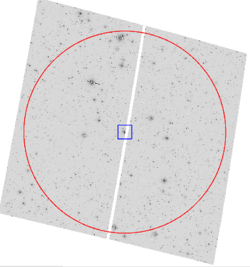
Figure 1: ACS/WFC image of Pluto and its stability region on UT 2005 May 15. The image has been corrected for the geometric distortion of the ACS and rotated so that north is up and east to the left. The ACS/WFC consists of two independent $4096\times 2048$-pixel CCDs butted together to form an effective $4096\times 4096$-pixel CCD with an approximately 50-pixel gap separating the two chips. The large field of view of the ACS/WFC ($202\arcsec\times 202\arcsec$) allowed Pluto’s entire stability zone, delineated by the large circle, to be imaged in a single exposure. The square at the center of the image represents the approximate size and location of the image in Fig. 2.

We conducted a search for additional satellites of Pluto using the F606W filter (“broad V”) in the Wide Field Channel (WFC) of the Advanced Camera for Surveys (ACS) on the Hubble Space Telescope (HST ) during two separate visits on UT 2005 May 15 and UT 2005 May 18 (Guest Observer program 10427). Observational details can be found in Table 1. The ACS/WFC has a field of view of $202\arcsec\times 202\arcsec$ with a plate scale of 0$\farcs$049 pixel^-1. This is well-matched to the angular size of Pluto’s stability region (185″ in angular diameter, as seen from Earth in May 2005), allowing the entire stability region to be imaged in a single HST pointing. A total of five images were obtained per HST visit: one short (0.5 sec) exposure with Pluto and Charon unsaturated and four long (475 sec) exposures. Pluto’s apparent motion, seen from HST and averaged over the visibility period, is 4$\farcs$2 h^-1. This caused stars to appear as streaks $\sim$11 pixels long, while unresolved objects moving with Pluto appeared as point sources in all four long images. A sample long exposure from this dataset can be seen in Fig. 1.

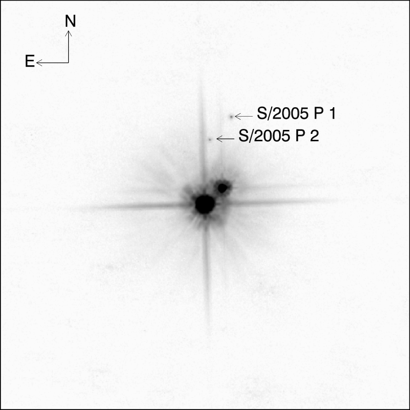
Figure 2: Drizzle combined ACS/HRC image of the Pluto system on 2006 February 15. This image shows a 512x512 pixel region near the center of the ACS/HRC detector. Pluto is centered on the image, while Charon is located 0$\farcs$77 from Pluto at a position angle of 313^∘. P1 (2$\farcs$86 from Pluto at a position angle of 343^∘) and P2 (2$\farcs$03 from Pluto at a position angle of 356^∘) can be clearly seen. No other satellites are detected.

With the detection of two additional satellites of Pluto in the ACS/WFC observations (Weaver et al., 2006), we obtained two additional HST visits to the Pluto system on 2006 February 15 and 2006 March 2 from the Director’s Discretionary Time (GO/DD program 10774). These observations were designed to confirm the existance of the two satellites (Mutchler et al., 2006) and were obtained using the ACS High Resolution Channel (HRC). The observations in February 2006 consisted of four 475-second integrations taken with the F606W filter with additional 1-second integrations (to allow for accurate image registration with Pluto and Charon unsaturated) at each position in a four point dither pattern. The final drizzle-combined image from the February 15, 2006 observations, with labels indicating the positions of S/2005 P 1 and S/2005 P 2, is shown in Fig. 2.

The observations in March 2006 were also designed to measure the B V colors of the satellites, and therefore alternated between 145-second integrations using the F606W filter and 475-second integrations using the F435W (Johnson B) filter. As such, the March 2 observations are less sensitive to faint satellites and were not used in the subsequent analysis. Some observational details about the ACS/HRC observations are also presented in Table 1.

3 Data Analysis

To estimate the sensitivity of our satellite search using the May 2005 ACS/WFC data, we generated synthetic point-spread functions (PSFs) at 400 locations in the plane of the sky using the Tiny Tim v6.3 software package (Krist & Hook, 2004), with the assumption that the sources have the same spectral distribution as the Sun. These PSFs were randomly-spaced in separation and position angle from Pluto and were scaled to uniformly span the range in WFC STMAG magnitudes of 25.5–29.5. To ensure proper sub-pixel alignment of the synthetic PSFs in the geometrically-distorted ACS images (i.e. FLT images) the PSFs were subsampled by a factor of five, resampled at the proper pixel locations, rebinned to normal size, and then convolved with the CCD charge diffusion kernel generated by the Tiny Tim program. Independent Poisson noise was applied to the synthetic PSFs before they were added, at the appropriate locations, to each of the four deep (475-second) exposures in the two ACS/WFC visits. The four images were then “drizzled” together using the “Multidrizzle” procedure supplied with the PyRAF software package (Koekemoer et al., 2002). In the drizzle procedure, the individual images are corrected for the geometric distortion of the ACS instrument, rotated so that north is up and east to the left, sky background subtracted, co-registered relative to Pluto, and combined using a median filter. In addition, pixels that have anomalously low sensitivity, that have high dark counts, or are saturated are excluded. The median combination removes artifacts, such as cosmic ray events or star trails, that do not appear in same position on the plane of the sky in at least two of the images. We then visually searched the final drizzle-combined image for objects (real or synthetic) with a PSF-like appearance.

Adding synthetic PSFs to the data before conducting the actual satellite search results in a more accurate estimate of the limiting magnitude of the search (since the conditions during the satellite search and the limiting magnitude estimation are identical). However, there is a small chance that one of the synthetic PSFs will be coincident with a real source, thus preventing the detection of the real source. Given the size of the ACS/WFC images and the relatively compact nature of the ACS/WFC PSF ($0.796\pm 0.003$ of the total flux from a point source is contained within a circle of radius 3 pixels for the ACS/WFC using the F606W filter Sirianni et al. (2005)), only 0.06% of the pixels in the ACS/WFC images change by more than 0.1 times the standard deviation in the sky background when the synthetic PSFs are added. Thus, we feel the benefit of obtaining a more accurate estimate of the limiting magnitude vastly outweighs the small risk of masking a real object with a synthetic PSF.

Visual identification of point sources is generally more reliable than identification by automated detection algorithms. However, it can also be more subjective and prone to operator error/fatigue. To minimize the possibility that a bona fide satellite of Pluto would be missed on account of operator error or some systematic error introduced via the drizzle analysis procedure, the data were searched a second time using an independent technique: the four deep exposures were manually co-registered, displayed to the screen, and then cycled rapidly between images at roughly 15 frames per second. As a result, stars would appear as trails moving through the displayed region and cosmic ray events and bad pixels would appear and disappear. Objects co-moving with Pluto (whether real satellites or synthetic PSFs) would appear in the same location in each of the four frames. Although this technique proved to be somewhat less sensitive than the drizzle combination technique, it yielded consistent results.

The field of view of the ACS/HRC is $29\arcsec\times 26\arcsec$, compared to $202\arcsec\times 202\arcsec$ with the ACS/WFC. With the smaller field of view, there is an increased risk that a synthetic PSF added to the data will be coincident with a real source in the data, thus preventing the detection of the real source. To avoid this possibility, data from the February 2006 ACS/HRC observations were first searched for satellites using the drizzle technique without the addition of synthetic PSFs. The data were then analyzed a second time, this time with synthetic PSFs added to provide an estimate of the sensitivity. A total of 200 PSFs, uniformly spaced between magnitudes 24.5 and 28.5, were added at random locations in each of two annuli centered on Pluto: one extending from 1″–3″ and the other from 3″–5″. Since placing so many synthetic PSFs in such a small area would result in a high probability of overlapping PSFs, the ACS/HRC data was analyzed 10 separate times, with only 20 randomly-selected PSFs in each annulus for each analysis run. After the synthetic PSFs were added, the ACS/HRC images were drizzle-combined and the resulting image was visually inspected for point sources in a manner similar to the ACS/WFC images.

Finally, to estimate the limiting magnitude within 1″ of Pluto, we placed 12 synthetic PSFs in a ring at an angular distance of 0$\farcs$5 from Pluto, using the techniques described above. The magnitude of the individual PSFs in the ring pattern was then varied until at least one of the PSFs could no longer be easily identified. Although this technique is not as statistically rigorous, it provides a reasonable estimate of the limiting magnitude in this region. Scattered light from Pluto prevents us from assigning meaningful upper limits within $\sim$0$\farcs$3 of Pluto.

4 Results and Discussion

As mentioned above, two satellites of Pluto, provisionally designated S/2005 P 1 and S/2005 P 2 (hereafter P1 and P2), were discovered during the analysis of the May 2005 ACS/WFC images (Weaver et al., 2006). During the discovery epoch, P1 had an apparent magnitude of $m_{{}_{V}}=22.93\pm 0.12$ and P2 had an apparent magnitude of $m_{{}_{V}}=23.38\pm 0.17$ (Weaver et al., 2006). Analysis of the discovery observations and archival HST observations yielded provisional orbits with semi-major axes of $64,780\pm 88$ km for P1 and $48,675\pm 121$ km for P2 (Buie et al., 2006). The orbits of P1 and P2 are circular (or nearly so) and co-planar with Pluto’s other large moon, Charon, implying these moons share a giant impact origin (Stern et al., 2006a). This hypothesis is supported by the observation that P1 and P2 are essentially neutral in color with B V values of $0.653\pm 0.026$ for P 1 and $0.654\pm 0.065$ for P2 (Stern et al., 2006b). No other satellites were detected, out to the edge of Pluto’s stability region.

The efficiency of detecting the synthetic point sources planted in the ACS images is used to estimate the sensitivity of our search. The detection efficiency, as a function of PSF magnitude (in the F606W passband), is shown in Fig. 3. Defining the limiting magnitude to be the level at which the detection efficiency drops to 90%, we find that the limiting magnitude, in the ACS/WFC F606W passband and using the STMAG magnitude system (Koornneef et al., 1986), of our search is $m_{{}_{F606W}}=27.5$. If we adopt a less stringent definition of limiting magnitude as the magnitude where the detection efficiency drops below 50% (Harris, 1990), then the limiting magnitude of our search is $m_{{}_{F606W}}=26.9$.

Both Pluto and Charon are severely over-exposed in the 475-second integrations. Scattered light from these objects significantly degrades the sensitivity of the ACS/WFC satellite search within 5″ ($1.1\times 10^{5}$ km) of Pluto. Since the plate scale of the ACS High Resolution Channel (HRC) is roughly twice that of the ACS/WFC (the ACS/HRC platescale is $\sim$0$\farcs$025/pixel versus $\sim$0$\farcs$049/pixel for the ACS/WFC), it is less severely affected by scattered light from Pluto and Charon, and so the February 2006 ACS/HRC observations were used to search for potential satellites within 5″ Pluto. Between 1″–3″ (a projected distance of $2.3\times 10^{4}$–$6.9\times 10^{4}$ km) the 90%-confidence limiting magnitude is $m_{{}_{F606W}}=25.8$ ($m_{{}_{F606W}}=27.0$ for 50%-confidence), while between 3″–5″ ($6.9\times 10^{4}$–$1.1\times 10^{5}$ km) from Pluto the 90%-confidence limiting magnitude is $m_{{}_{F606W}}=26.5$ ($m_{{}_{F606W}}=27.3$ for 50%-confidence). Between 0$\farcs$3–1″ ($6.9\times 10^{3}$–$2.3\times 10^{4}$ km) from Pluto the 90%-confidence limiting magnitude is $m_{{}_{F606W}}=24$.

4.1 Conversion of STMAG to V magnitudes

The above magnitude limits use the STMAG magnitude system with the ACS/WFC and HRC F606W filters (Koornneef et al., 1986). These can be converted into standard Johnson V magnitudes via the following equation:

$$m_{{}_{V}}=m_{{}_{F606W}}+c_{{}_{0}}+c_{{}_{1}}(\bv)+c_{{}_{2}}(\bv)^{2}-Z_{{}_{ST}}$$ (2)

where $m_{{}_{F606W}}$ is the magnitude in the F606W passband using the STMAG system and $\bv$ is the object’s color in the Johnson system. The coefficients $c_{{}_{0}}$, $c_{{}_{1}}$, and $c_{{}_{2}}$ as well as the magnitude system zero point, $Z_{{}_{ST}}$ are given by (Sirianni et al., 2005). Objects in the outer solar system exhibit a wide range of B V colors, e.g. $\bv=0.65$ for P1 and P2 (Stern et al., 2006b) and $\bv=1.23$ for 5145 Pholus (Barucci et al., 2005). Since all three of Pluto’s known satellites exhibit roughly neutral colors (Charon has a B V of 0.71 (Buie et al., 1997) compared with the solar B V color of 0.67 (Hardorp, 1980)) it is reasonable to assume that any as yet undetected satellites of Pluto would have $\bv\approx 0.7$. Substituting the appropriate values into Eq. 2, we find $m_{{}_{V}}-m_{{}_{F606W}}=-0.096$ for the ACS/WFC and $m_{{}_{V}}-m_{{}_{F606W}}=-0.092$ for the ACS/HRC. If, instead, the undetected satellites have extremely red B V colors (i.e. similar to 5145 Pholus), then $m_{{}_{V}}$ would be $\approx 0.2$ mag fainter. The limiting magnitudes of the satellite search, converted into Johnson V magnitudes are given in Table 2.

4.2 Limiting satellite diameter

Once a limiting magnitude has been determined, the diameter, in kilometers, of a spherical satellite, in the absence of significant limb darkening, can be derived via the following equation (Russell, 1916):

$$d=2.99\times 10^{8}\,r\Delta p_{{}_{V}}^{-1/2}\,10^{(m_{\sun}-m_{{}_{V}}+\beta\alpha)/5}$$ (3)

where $r$ and $\Delta$ are the distances from Pluto to the Sun and Pluto to the Earth, respectively, in units of AU; $p_{{}_{V}}$ is the geometric visual albedo; $m_{\sun}=-26.75$ is the V magnitude of the Sun at a distance of 1 AU (Colina et al., 1996); $\beta$ is the phase law (in mag deg^-1); and $\alpha$ is the phase angle of the object (i.e. the Sun-object-observer angle). We assume the phase law for potential satellites identical to that for Charon, i.e. $\beta=0.0866\pm 0.0078$ mag deg^-1 (Buie et al., 1997).

Thus, assuming a very dark albedo of $p_{{}_{V}}=0.04$, comparable with cometary nuclei (Lamy et al., 2004), we can rule out, at the 90%-level of confidence, the existence of additional satellites in the Pluto system larger than 49.4 km in diameter over the span of separations from Pluto of 1″–3″, 36.1 km over the span of 3″–5″, and 28.6 km in diameter at separations of more than 5″ from Pluto. If, instead, we assume that potential satellites are as reflective as Charon, i.e. having $p_{{}_{V}}=0.38$ (Buie et al., 1997), then we can rule out satellites in these three regions larger than 16.0, 11.7, and 9.3 km in diameter, respectively. Within 1″of Pluto, the limiting diameters are 115 km for an albedo of $p_{{}_{V}}=0.04$ and 37 km for an albedo of $p_{{}_{V}}=0.38$. Our limiting diameters in this region are comparable to the limits obtained by Stern et al. (1994) using dynamical arguments and an assumed orbital eccentricity of Charon of $10^{-4}$, which is reasonable given the uncertainty of 7x10^-5 in the recently published finding of zero eccentricity in the orbit of Charon (Buie et al., 2006). These results are summarized in Table 2, and the limiting diameter for Plutonian satellites for the four regions, as a function of satellite albedo, is shown in Fig. 4.

The above discussion has assumed a zero-amplitude light curve for potential satellites. While Charon exhibits a relatively small light curve amplitude (defined as the difference between maximum and minimum magnitude and not the absolute deviation from the mean) of only 0.08 mag in V (Buie et al., 1997), other Kuiper belt objects (KBOs) exhibit much larger light curve effects (Trilling & Bernstein, 2006). An extreme example is the KBO 2001 QG₂₉₈, which exhibits a light curve with an amplitude of 1.14 mag in R (Sheppard & Jewitt, 2004). If an object with a similarly extreme light curve exists within the Pluto system and was at the minimum of its light curve during both of the ACS/WFC (if the object is located more than 5″ from Pluto) or ACS/HRC visits (if the object is within 5″ of Pluto), it could have escaped detection, though its peak brightness would be nearly 3 times greater than the upper limits quoted above. In this pathological case, the length of the satellite in two dimensions could be as large as the limiting diameters quoted above, while the length in the third dimension could be up to a factor of 3 greater. The effective diameter of such a cigar-shaped satellite would be approximately 44% greater than the above size limits.

The 90%-confidence limit of $m_{{}_{V}}=25.7$ at separations greater than 1″ from Pluto places an upper limit of roughly 49 km on the diameter of undetected satellites in this region. Assuming bulk properties (albedo, light curve, phase effect, density, etc) similar to Pluto’s smallest known moon, P2, potential undetected satellites in this region must be less than 40% the size of P2 with a mass of 2.5% that of P2. Such a small satellite would be unable to strongly perturb the orbits of either P1 or P2, and therefore the proposed circular, or near-circular, orbits of P1 and P2 (Weaver et al., 2006; Buie et al., 2006) do not necessarily preclude the existence of other very small satellites in the Pluto system. Finally, we note that both P1 and P2 appear to be in, or near, mean-motion resonance with Charon, and therefore, we suggest that satellites below the detection limit of our search, may occupy the other mean-motion resonances. We suggest further observations with greater sensitivity to investigate this possibility.

Table 1: Observational Parameters

Observation Date (UT)	Channel	Filter	r (AU)	$\Delta$ (AU)	Phase Angle ($\alpha$)
2005 May 15.045	ACS/WFC	F606W	30.95	30.07	0.96∘
2005 May 18.141	ACS/WFC	F606W	30.95	30.05	0.88∘
2006 Feb 15.659	ACS/HRC	F606W	31.07	31.54	1.59∘
2006 Mar 2.747	ACS/HRC	F475W and F606W	31.08	31.31	1.77∘

Table 2: Limits on Additional Satellites

	Angular Separation from Pluto
	0$\farcs$3–1″	1″–3″	3″–5″	$>$5″
Projected Distance (km)	$6.9\times 10^{3}$–$2.3\times 10^{4}$	$2.3\times 10^{4}$–$6.9\times 10^{4}$	$6.9\times 10^{4}$–$1.1\times 10^{5}$	$>1.1\times 10^{5}$
50%-Conf. Lim. V Mag		26.9	27.2	27.4
90%-Conf. Lim. V Mag	24.	25.7	26.4	26.8
Max. Diameter (km)	37	16.0	11.7	9.3
$\rho_{{}_{V}}=0.38$
Max. Diameter (km)	115	49.4	36.1	28.6
$\rho_{{}_{V}}=0.04$

Figure 3: Detection efficiency as a function of STMAG magnitude for PSFs more than 5″ from Pluto. Points on the graph represent the running average of the detection efficiency, in bins 0.5 mag in width centered on points spaced every 0.01 mag. A total of 400 synthetic PSFs, distributed randomly in the plane of the sky and uniformly in flux between magnitudes 25.5 and 29.5, were added to each of the four ACS/WFC images per HST visit. Data from each visit were analyzed twice. The 90% and 50% level of detection efficiency are marked by horizontal dotted lines. The 90%-confidence magnitude limit is $m_{lim,90\%}=26.9$, while the 50%-confidence magnitude limit, i.e., the limiting magnitude as defined by Harris (1990), is $m_{lim,50\%}=27.5$. These magnitude limits use the STMAG magnitude system with the F606W passband. Magnitude limits transformed into the Johnson V passband are presented in Table 2.

Figure 4: Maximum diameter of undiscovered satellites of Pluto, as a function of geometric albedo, assuming a light curve amplitude of zero and a limiting magnitude defined by the 90% detection efficiency criterion. Filled circles mark the locations of $p_{{}_{V}}=0.04$ (comet-like albedo) and $p_{{}_{V}}=0.38$ (Charon-like albedo).

References

- Barucci et al. (2005) Barucci, M. A., Belskaya, I. N., Fulchignoni, M., & Birlan, M. 2005, AJ, 130, 1291
- Buie et al. (2006) Buie, M. W., Grundy, W. M., Young, E. F., Young, L. A., & Stern, S. A. 2006, AJ, in press
- Buie et al. (1997) Buie, M. W., Tholen, D. J., & Wasserman, L. H. 1997, Icarus, 125, 233
- Carruba et al. (2002) Carruba, V., Burns, J. A., Nicholson, P. D., & Gladman, B. J. 2002, Icarus, 158, 434
- Christy & Harrington (1978) Christy, J. W. & Harrington, R. S. 1978, AJ, 83, 1005
- Colina et al. (1996) Colina, L., Bohlin, R. C., & Castelli, F. 1996, AJ, 112, 307
- Hamilton & Burns (1992) Hamilton, D. P. & Burns, J. A. 1992, Icarus, 96, 43
- Hamilton & Krivov (1997) Hamilton, D. P. & Krivov, A. V. 1997, Icarus, 128, 241
- Hardorp (1980) Hardorp, J. 1980, A&A, 91, 221
- Harris (1990) Harris, W. E. 1990, PASP, 102, 949
- Koekemoer et al. (2002) Koekemoer, A. M., Fruchter, A. S., Hook, R., & Hack, W. 2002, in HST Calibration Workshop, 337
- Koornneef et al. (1986) Koornneef, J., Bohlin, R., Buser, R., Horne, K., & Turnshek, D. 1986, Highlights in Astronomy, 7, 833
- Krist & Hook (2004) Krist, J. & Hook, R. 2004, The Tiny Tim User’s Guide version 6.3, http://www.stsci.edu/software/tinytim/tinytim.pdf
- Kuiper (1961) Kuiper, G. P. 1961, Limits of Completeness (Planets and Satellites), 575–591
- Lamy et al. (2004) Lamy, P., Toth, I., Fernández, Y., & Weaver, H. 2004, Comets II (University of Arizona Press), 223–264
- Marcialis (1997) Marcialis, R. L. 1997, The First 50 Years of Pluto-Charon Research (Pluto and Charon), 27–83
- Marcialis & Merline (1998) Marcialis, R. L. & Merline, W. J. 1998, Bulletin of the American Astronomical Society, 30, 1109
- Mutchler et al. (2006) Mutchler, M. J., Steffl, A. J., Weaver, H. A., Stern, S. A., Buie, M. W., Merline, W. J., Spencer, J. R., Young, E. F., & Young, L. A. 2006, IAU Circ., 8676, 1
- Nesvorný et al. (2003) Nesvorný, D., Alvarellos, J. L. A., Dones, L., & Levison, H. F. 2003, AJ, 126, 398
- Nicholson & Gladman (2006) Nicholson, P. D. & Gladman, B. J. 2006, Icarus, 181, 218
- Reaves (1997) Reaves, G. 1997, Pluto and Charon (University of Arizona Press), 3–25
- Russell (1916) Russell, H. N. 1916, ApJ, 43, 173
- Sheppard & Jewitt (2004) Sheppard, S. S. & Jewitt, D. 2004, AJ, 127, 3023
- Sirianni et al. (2005) Sirianni, M., Jee, M. J., Benítez, N., Blakeslee, J. P., Martel, A. R., Meurer, G., Clampin, M., De Marchi, G., Ford, H. C., Gilliland, R., Hartig, G. F., Illingworth, G. D., Mack, J., & McCann, W. J. 2005, PASP, 117, 1049
- Slipher (1930) Slipher, V. M. 1930, Lowell Obs. Observation Circ., March 13
- Stern et al. (1994) Stern, S. A., Parker, J. W., Duncan, M. J., Snowdall, J. C. J., & Levison, H. F. 1994, Icarus, 108, 234
- Stern et al. (1991) Stern, S. A., Parker, J. W., Fesen, R. A., Barker, E. S., & Trafton, L. M. 1991, Icarus, 94, 246
- Stern et al. (2006b) Stern, S. A., Weaver, H. A., Mutchler, M. J., Steffl, A. J., Merline, W. J., Spencer, J. R., Buie, M. W., Young, E. F., & Young, L. A. 2006b, IAU Circ., 8686, 1
- Stern et al. (2006a) Stern, S. A., Weaver, H. A., Steffl, A. J., Mutchler, M. J., Merline, W. J., Buie, M. W., Young, E. F., Young, L. A., & Spencer, J. R. 2006a, Nature, 439, 946
- Szebehely (1967) Szebehely, V. 1967, Theory of Orbits. The Restricted Problem of Three Bodies (New York: Academic Press)
- Szebehely (1978) —. 1978, Celestial Mechanics, 18, 383
- Tombaugh (1960) Tombaugh, C. W. 1960, S&T, 19, 264
- Trilling & Bernstein (2006) Trilling, D. E. & Bernstein, G. M. 2006, AJ, 131, 1149
- Weaver et al. (2006) Weaver, H. A., Stern, S. A., Mutchler, M. J., Steffl, A. J., Buie, M. W., Merline, W. J., Spencer, J. R., Young, E. F., & Young, L. A. 2006, Nature, 439, 943