Relativistic MHD Simulations of Jets with Toroidal Magnetic Fields.

Abstract

This paper presents an application of the recent relativistic HLLC approximate Riemann solver by Mignone & Bodo to magnetized flows with vanishing normal component of the magnetic field. The numerical scheme is validated in two dimensions by investigating the propagation of axisymmetric jets with toroidal magnetic fields. The selected jet models show that the HLLC solver yields sharper resolution of contact and shear waves and better convergence properties over the traditional HLL approach.

1 Introduction

Jets are one of the fundamental components of radio-loud active galactic nuclei (AGN). Although different in detail, they all share the property of being relativistic on the parsec scale and of carrying magnetic fields that may be dynamically important. Observations of their non-thermal synchrotron radiation, in fact, require the presence of a magnetic field and the high degree of polarization observed indicates the presence of some large scale structure in the field.

Theoretical investigations require, therefore, a relativistic MHD description of such objects. In this effort, recent numerical simulations [Komissarov (1999b), Leismann et al. (2005)] have turned out as efficient investigation tools in understanding many aspects of the jet evolution. This, in turn, justifies recent and new efforts to extend existing gas-dynamical Godunov-type codes to the relativistic regime, see K99a, Balsara01, dZBL03, and the extensive review by MM03. In this perspective, we extend the recently derived relativistic hydrodynamical HLLC Riemann solver [Mignone & Bodo (2005)] to the magnetic case, with vanishing normal component of the magnetic field. The novel numerical scheme is then applied to the propagation of relativistic jets in presence of toroidal magnetic fields. The paper is organized as follows: in §2 we give the relevant relativistic MHD equations, in §3 we briefly review the approximate Riemann solver. Finally, in §4 we discuss the astrophysical jet applications.

2 RMHD Equations

The motion of a magnetized, ideal relativistic fluid is governed by the system of conservation laws [Anile (1989)]

$$\frac{\partial\mathbf{U}}{\partial t}+\sum_{d}\frac{\partial\mathbf{F}^{d}}{\partial x^{d}}=0\;,$$ (1)

where $d=x,y,z$ and $\mathbf{U}=(D,m_{k},B_{k},E)$ is the vector of conservative variables with components given, respectively, by the laboratory density $D$, the three components of momentum $m_{k}$ and magnetic field $B_{k}$ ($k=x,y,z$) and the total energy density $E$. $\mathbf{F}^{k}$ are the fluxes along the $x^{k}$ direction; for $k=x$ one has

$$\mathbf{F}^{x}=\left[Dv_{x},\,m_{k}v_{x}-B_{x}\left(\frac{B_{k}}{\gamma^{2}}+(\mathbf{v}\cdot\mathbf{B})v^{k}\right)+p\delta_{xk},\,B_{k}v_{x}-B_{x}v_{k},\,m_{x}\right]\,,\quad$$ (2)

where $p=p_{g}+|\mathbf{B}|^{2}/(2\gamma^{2})+(\mathbf{v}\cdot\mathbf{B})^{2}/2$ is the total pressure, $p_{g}$ is the thermal (gas) pressure and $\mathbf{v}\equiv(v_{x},v_{y},v_{z})$ is the fluid three-velocity. The Lorentz factor is denoted with $\gamma$. Expressions for $\mathbf{F}^{y}(\mathbf{U})$ and $\mathbf{F}^{z}(\mathbf{U})$ follow by cyclic permutations of the indexes.

Introducing the primitive flow variables $\mathbf{V}=(\rho,\mathbf{v},p_{g},\mathbf{B})$, one has

$$D = \rho\gamma\;,$$ (3)

$$m_{k} = (\rho h\gamma^{2}+|\mathbf{B}|^{2})v_{k}-(\mathbf{v}\cdot\mathbf{B})B_{k}\;,$$ (4)

$$E = \displaystyle\rho h\gamma^{2}-p_{g}+\frac{|\mathbf{B}|^{2}}{2}+\frac{|\mathbf{v}|^{2}|\mathbf{B}|^{2}-(\mathbf{v}\cdot\mathbf{B})^{2}}{2}\;,$$ (5)

where $\rho$ and $h$ are, respectively, the rest-mass density and specific enthalpy of the fluid. An additional equation of state is necessary to close the system (1). Throughout the following we will assume a constant $\Gamma$-law, with specific enthalpy given by

$$h=1+\frac{\Gamma}{\Gamma-1}\frac{p_{g}}{\rho}\;,$$ (6)

where $\Gamma$ is the constant specific heat ratio.

2.1 Recovering primitive variables

Godunov-type codes [Godunov (1959)] are based on a conservative formulation where laboratory density, momentum, energy and magnetic fields are evolved in time. On the other hand, primitive variables, $\mathbf{V}=(\rho,\mathbf{v},p_{g},\mathbf{B})$, are required for the computation of the fluxes (eq. 2) and more convenient for interpolation purposes.

This task requires the solution of the nonlinear equation

$$f(W)\equiv W-p_{g}+\left(1-\frac{1}{2{\gamma}^{2}}\right)|\mathbf{B}|^{2}-E-\frac{S^{2}}{2W^{2}}=0\;$$ (7)

where $W=\rho h\gamma^{2}$, $S=\mathbf{m}\cdot\mathbf{B}$. Equation (7) follows directly from equation (5) together with (4). Since, at the beginning of a time step $E$, $\mathbf{B}$ and $\mathbf{m}$ are known quantities, both $\gamma$ and $p_{g}$ may be expressed in terms of $W$ alone from

$$|\mathbf{m}|^{2}=\left(W+|\mathbf{B}|^{2}\right)^{2}\left(1-\frac{1}{\gamma^{2}}\right)-\frac{S^{2}}{W^{2}}\left(|\mathbf{B}|^{2}+2W\right)\;,$$ (8)

and from the equation of state (6) using $\rho=D/\gamma$. Equation (7) can be solved by any standard root finding algorithm. Once $W$ has been found, the Lorentz factor is easily found from (8), the thermal pressure from (6) and velocities are found by inverting equation (4):

$$v_{k}=\frac{1}{W+|\mathbf{B}|^{2}}\left(m_{k}+\frac{S}{W}B_{k}\right)$$ (9)

Finally, equation (3) is used to determine the proper density $\rho$.

3 A relativistic HLLC Riemann solver

In the traditional Godunov approach [Godunov (1959)], the conservation laws (1) are advanced in time by solving, at each zone interface $x_{i+\frac{1}{2}}$, a Riemann problem with initial condition

$$\mathbf{U}(x,0)=\left\{\begin{array}[]{ccc}\mathbf{U}_{L,i+\frac{1}{2}}&\quad\textrm{if}&x<x_{i+\frac{1}{2}}\,,\\ \vskip 6.0pt plus 2.0pt minus 2.0pt\cr\mathbf{U}_{R,i+\frac{1}{2}}&\quad\textrm{if}&x>x_{i+\frac{1}{2}}\,,\\ \vskip 6.0pt plus 2.0pt minus 2.0pt\cr\end{array}\right.$$ (10)

where $\mathbf{U}_{L,i+\frac{1}{2}}$ and $\mathbf{U}_{R,i+\frac{1}{2}}$ are the left and right edge values at zone interfaces. The exact solution to the Riemann problem for the relativistic MHD equations has been recently derived by GR05. As in the classical case, a seven-wave pattern emerges from the decay of an initial discontinuity separating two constant states. The resulting structure can be found by iterative techniques and it can be quite involved.

For the present purposes, however, we will be concerned with the special case where the component of magnetic field normal to a zone interface vanishes. Under this condition, a degeneracy occurs where the tangential, Alfvén and slow waves all propagate at the speed of the fluid and the solution simplifies to a three-wave pattern. In this special situation, the relativistic HLLC approximate Riemann solver originally derived for the gas-dynamical equations by TSS94 and recently extended to the relativistic regime by MB05 (paper I henceforth), can still be applied with minor modifications. This statement stems from the fact that both state and flux vectors on either side of the tangential discontinuity (denoted with the $*$ superscript) retain the same form as in the non-magnetized case:

$$\mathbf{U}^{*}_{L,R}=\left(D^{*},\,m^{*}_{x},\,m^{*}_{y},\,m^{*}_{z},\,B^{*}_{y},\,B^{*}_{z},\,E^{*}\right)_{L,R}\,,$$ (11)

$$\mathbf{F}^{*}_{L,R}=\left(D^{*}v^{*}_{x},\,m^{*}_{x}v^{*}_{x}+p^{*},\,m^{*}_{y}v^{*}_{x},\,m^{*}_{z}v^{*}_{x},\,B^{*}_{y}v^{*}_{x},\,B^{*}_{z}v^{*}_{x},\,m^{*}_{x}\right)_{L,R}\,,$$ (12)

where we can still set $m_{x}^{*}=(E^{*}+p^{*})v_{x}^{*}$. Total pressure and normal velocity are continuous across the middle wave, i.e. $p^{*}_{L}=p^{*}_{R}$, $v^{*}_{x,L}=v^{*}_{x,R}$. The method of solution is thus entirely analogous to the strategy shown in paper I and we will not repeat it here. The two additional components related to the presence of transverse magnetic field are decoupled from the rest and can be solved without additional complications. Once $v^{*}_{x}$ has been found, in fact, we use the jump conditions to get

$$B^{*}_{y,z}=\displaystyle\frac{\lambda-v_{x}}{\lambda-v_{x}^{*}}\,B_{y,z}$$ (13)

from the pre-shock states.

Finally, we need an estimate for the outermost right and left-going fast wave speeds, $\lambda_{R}$ and $\lambda_{L}$. These two signal velocities may be found by exploiting the characteristic decomposition of the RMHD equation, extensively analyzed by AP87 and Anile89. In the general case, the fast and slow magneto-sonic waves satisfy a quartic equation solvable by means of numerical and analytical methods, e.g. dZBL03. For vanishing normal component of the magnetic field, however, the two roots corresponding to the degenerate slow waves have the trivial solution $\lambda=v_{x}$, whereas the fast speeds satisfy the following quadratic:

$$(\lambda-v_{x})^{2}=\sigma_{s}(1-\lambda^{2})\,,$$ (14)

with

$$\sigma_{s}=\frac{B^{2}/\gamma^{2}+\rho hc_{s}^{2}+(\mathbf{v}\cdot\mathbf{B})^{2}(1-c_{s}^{2})}{\rho h(1-c_{s}^{2})\gamma^{2}}$$ (15)

where $c_{s}=\sqrt{\Gamma p/(\rho h)}$ is the speed of sound. The solutions of (14) are used to provide suitable guesses for the outermost signal velocities in our HLLC Riemann solver. As in paper I, we set

$$\lambda_{L}=\min\big{(}\lambda_{-}(\mathbf{V}_{L}),\lambda_{-}(\mathbf{V}_{R})\big{)}\;,\quad\lambda_{R}=\max\big{(}\lambda_{+}(\mathbf{V}_{L}),\lambda_{+}(\mathbf{V}_{R})\big{)}\;,$$ (16)

where $\lambda_{-}$ ($\lambda_{+}$) is the smallest (biggest) fast wave speed.

4 Code Validation

Spatial and temporal discretization of equations (1) is based on the second-order Hancock predictor step already described in paper I. For the sake of conciseness we will not repeat it here.

4.1 A Shock-Tube Example

As an illustrative test, we consider an initial discontinuity separating two constant left and right states given by

$$\big{(}\rho,p_{g},v_{x},v_{y},v_{z},B_{y},B_{z}\big{)}=\left\{\begin{array}[]{cccccccc}\big{(}1,&30,&0,&0,&0,&20,&0\big{)}_{L}&\textrm{for}\quad x<0.5\,,\\ \vskip 6.0pt plus 2.0pt minus 2.0pt\cr\big{(}0.1,&1,&0,&0,&0,&0,&0\big{)}_{R}&\textrm{for}\quad x>0.5\,.\\ \vskip 6.0pt plus 2.0pt minus 2.0pt\cr\end{array}\right.$$ (17)

Figure 1: Computed profiles (symbols) and exact solution (solid line) for the first test problem. The second-order scheme with the HLLC Rieman solver has been employed on $1600$ zones. The final integration time is $t=0.25$; the Courant number is $0.5$. The solution is comprised of a left-going fast rarefaction, a right-going tangential and shock waves moving close to each other.

The domain is the interval $[0,1]$ covered with $1600$ uniform computational cells. The ideal equation of state (6) is used with $\Gamma=4/3$. Figure (1) compares the result computed with the HLLC solver with the analytical solution (available from GR05), at the final time $t=0.25$. The breakup of the discontinuity results in a left-going fast rarefaction wave and a thin shell of high density material bounded by a tangential discontinuity and a gasdynamical shock propagating to the right. The total pressure and magnetic field are continuous through the contact and the shock wave, respectively. All discontinuities are correctly captured, with satisfactory resolutions: the tangential discontinuity and the shock smear out over $\sim 5\div 6$ and $4\div 5$ zones, respectively. Small overshoots appear at the tail of the rarefaction fan. A similar, perhaps more pronounced behavior is shown in the results by K99a who used a linearized, Roe-like Riemann solver. The relative error in the thin shell is $\lesssim 1\%$ for both pressure and density.

4.2 Axisymmetric Jet with Toroidal Magnetic Field

We now turn our attention to the propagation of a relativistic magnetized jet in cylindrical coordinates $(r,z)$. For the sake of comparison, we have implemented three models already discussed in literature. The first setup, denoted with $S1$, is model $A$ of K99b (K99 henceforth), the second and third setups, $S2$ and $S3$, are taken from models $C2\_10/3$ and $C2\_1/20$ of LAAM05 (L05 henceforth), respectively.

Model	$\rho_{j}$	$\rho_{e}$	$v_{j}$	$r_{m}$	$\bar{\beta}$	$\Gamma$	$\sigma$
$S1$	$1$	$10^{3}$	$\sqrt{0.99}$	$0.37$	$1$	$4/3$	$0.34$
$S2$	$10^{-2}$	$1$	$0.99$	$0.6$	$10/3$	$5/3$	$0.11$
$S3$	$10^{-2}$	$1$	$0.99$	$0.6$	$1/20$	$5/3$	$0.0017$

Table 1: Relevant parameters for models $S1$, $S2$ and $S3$ described in the text. From left to right: jet density, ambient medium density, beam velocity, magnetization radius, average magnetization, specific heat ratio and magnetic to rest mass energy ratio.

In all models, the static external medium has uniform density $\rho_{e}$ and zero magnetic field. At the inlet, $r\leq 1$ and $z=0$, a supersonic beam with uniform velocity $v_{j}$ (Lorentz factor $\gamma_{j}$) and density $\rho_{j}$ is injected with a toroidal magnetic field obeying

$$B_{\phi}(r)=\left\{\begin{array}[]{ccc}\gamma_{j}b_{m}r/r_{m}&\quad\textrm{if}&r<r_{m}\,,\\ \vskip 6.0pt plus 2.0pt minus 2.0pt\cr\gamma_{j}b_{m}r_{m}/r&\quad\textrm{if}&r_{m}<r<1\,,\\ \vskip 6.0pt plus 2.0pt minus 2.0pt\cr\end{array}\right.$$ (18)

where $r_{m}$ is the magnetization radius of the beam. The ideal equation of state (6) is used in all calculations. In model $S1$, we set $b_{m}=1$ and the thermal pressure inside the beam, $p_{j}$, is prescribed from the condition of hydromagnetic equilibrium,

$$p_{j}(r)=\left\{\begin{array}[]{ccc}p_{e}\left[\alpha+\frac{2}{\beta}\left(1-(r/r_{m})^{2}\right)\right]&\quad\textrm{if}&r<r_{m}\;,\\ \vskip 6.0pt plus 2.0pt minus 2.0pt\cr\alpha p_{e}&\quad\textrm{if}&r_{m}<r<1\;,\\ \vskip 6.0pt plus 2.0pt minus 2.0pt\cr\end{array}\right.$$ (19)

where $\alpha=1-r_{m}^{2}/\beta$, $\beta=0.34$ and $p_{e}=\beta b_{m}^{2}/2$ is the thermal pressure of the ambient medium. In models $S2$ and $S3$ $b_{m}$ is computed from the average magnetization parameter $\bar{\beta}$:

$$b_{m}=\sqrt{\frac{4p_{b}\bar{\beta}}{r_{m}^{2}(1-4\log r_{m})}}\,,$$ (20)

and the thermal pressure follows directly from the definition of the Mach number, i.e.

$$p_{j}=\frac{\rho_{j}v_{j}^{2}(\Gamma-1)}{\Gamma(\Gamma-1)M_{j}^{2}-\Gamma v_{j}^{2}}\,,$$ (21)

with $M_{j}=6$. The numerical values of the relevant parameters are given in Table 1. The simulations are performed on the physical domain $r\in[0,10.5]$, $z\in[0,50]$ using $20$ points per jet radius. The total grid size is $210\times 1000$.

For each model, we have carried two set of simulations: the first one employing the HLLC approximate Riemann solver described in §3 and the second one adopting the HLL scheme, also used in L05.

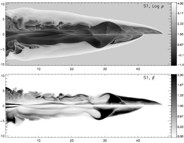
Figure 2: Model S1 at $t=100$. The top and bottom panels show, respectively, the density logarithms and magnetization parameter $\beta$ for the HLLC (upper half of each panel) and HLL (lower half of each panel) runs. Notice that the two panels use opposite color gradients. The grid resolution is $20$ zones per jet beam, giving a total grid size of $210$ (in $r$) and $1000$ zones (in $z$). Integration has been carried with CFL = 0.4 and the second-order Hancock scheme outlined in paper I.

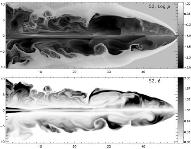
Figure 3: Model S2 at $t=126$. The top panel shows the density logarithm in the HLLC (upper half) and HLL (lower half) runs. The bottom panel shows the magnetization parameter in the HLLC (upper half) and HLL (lower half) runs. The final integration time is the same one as in L05.

Models $S1$ and $S2$ are characterized by a high Poynting flux $B^{2}_{\phi}v$ and tend to develop prominent nose cones due to the strong magnetic pinching. This is evident from Fig. (2) and (3), where the upper (lower) portion of each gray scale image refers to the HLLC (HLL) approximate Riemann solver at $t=100$ and $t=126$, respectively. The nose cone appears as the extended high pressure region bounded by the terminal conical shock (mach disk) and the bow shock. At the Mach disk, the beam is strongly decelerated and magnetic tension wards off sideways deflection of shocked material into the cocoon. The magnetization parameter, defined as $\beta=B_{\phi}^{2}/(2\gamma^{2}p_{g})$, is particularly strong in the cone above the symmetry axis. As pointed out by K99, morphological properties are prevalently dictated by the ratio of the kinetic energy flux to the Poynting flux, $\kappa=\rho_{j}h_{j}\gamma_{j}^{2}/B_{\phi}^{2}$, which determines the magnetization of shocked gas behind the terminal shock. An alternative parameter (L05) is the ratio of the magnetic energy density to the rest mass, $\sigma=B_{\phi}^{2}/(\gamma^{2}\rho)$: extended nose cones tend to form for low $\kappa$ (high $\sigma$), whereas familiar cocoon structures appear for high values of $\kappa$ (low $\sigma$), regardless of the jet magnetization parameter $\beta$. Values of $\sigma$ are reported in Table 1.

Figure 4: Jet head positions for model $S1$ computed for three different resolution runs: low ($105\times 500$), medium ($210\times 1000$) and high ($240\times 2000$). The HLLC runs are shown using, respectively, dotted, dashed and solid lines; for the HLL we use plus signs, triangles and squares.

The positions of the reverse shocks for the HLL and HLLC runs are, respectively, $z\sim 30$ and $z\sim 26$ in model $S1$, $z\sim 33$ and $z\sim 41$ in model $S2$. However, the most striking difference between the HLL and HLLC schemes is the jet propagation speed obtained from model $S1$. Indeed, at $t=100$ the head position in the HLLC run is $z\sim 47.6$ to be compared with a value of $z\sim 41.8$ obtained from the HLL integration. Note that the final integration time is not the same as in K99, where the simulation ends at a later time, $t=110$, yielding a head position value of $z\sim 46$, apparently more consistent with the HLL run. However, in order to further investigate these discrepancies, we carried out an additional set of simulations at half and twice the resolution. Figure (4) plots the jet head position as function of time for the three resolutions in consideration: low ($105\times 500$), medium ($210\times 1000$) and high ($420\times 2000$). The HLL scheme achieves the same convergence of the HLLC scheme only at high resolution, whereas the propagation speeds in the HLLC runs show to be by far less sensitive to the grid size.

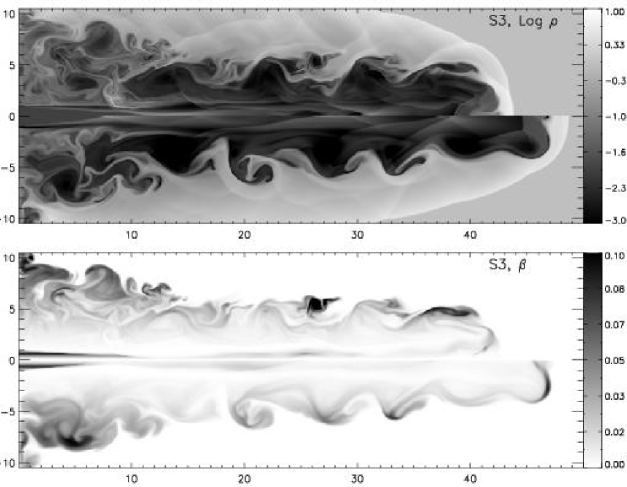
Figure 5: Model S3 at $t=126$. The final integration time is the same one used in L05. The meaning of the gray scale images in the same as in Fig. (2) and (3).

This disagreement is remarkably reduced in the second model $S2$, where the HLL runs shows a slightly higher propagation speed, but again more evident in model $S3$, although with an opposite trend. Once more we ascribe this behavior to resolution effects, based on the fact that the same model in L05 with twice the resolution (i.e. $40$ zones per beam radius instead of $20$) shows stronger affinities with the HLLC integration presented here.

When the HLLC solver is employed, the backflow turbulent patterns in the cocoon are better defined than with the HLL scheme, where the larger numerical viscosity inhibits the formation of small scale structure at lower resolution. This is corroborated by a simple qualitative comparison with the results of L05, who used twice the resolution employed here and the HLL solver. The small scale structural details provided by the HLLC approach appear to be almost equivalent even at half the resolution. This consideration together with the convergence test previously shown confirms, indeed, that the ability to describe tangential and shear waves largely improves the quality of solution, particularly in the multidimensional case.

Finally, we remind that the computational cost of the HLLC scheme over the traditional HLL Riemann solver is less than $7\%$ and we believe that this largely justifies its use in Godunov-type codes.

5 Discussion

Numerical simulations of relativistic magnetized jets with toroidal magnetic fields have been presented. The three models considered show formation of conspicuous nose cones and jet confinement with increasing magnetization. The morphological properties favorably compare with the results of previous investigators. Simulations have been conducted by using the recent relativistic hydrodynamics HLLC solver by Mignone & Bodo, opportunely extended to the special case of vanishing normal component of magnetic field. In order to assess the validity of the new algorithm, simulations have been directly compared with the traditional HLL Riemann solver [Del Zanna et al. (2003)]. It is found that the HLLC approach largely improves the quality of solution over the HLL scheme by considerably reducing the amount of numerical viscosity. This is manifested in a sharper resolution of fine scale structures in proximity of shear and tangential flows. Furthermore, convergence tests at different resolutions have shown that, with the HLLC scheme, the jet head position has little dependence on the grid size. This is a remarkable property for a shock-capturing scheme and has to be consolidated through further numerical testing. Generalization to the full relativistic MHD case is underway.

References

- Anile & Pennisi (1987) Anile, M., & Pennisi, S. 1987, Ann. Inst. Henri Poincaré, 46, 127
- Anile (1989) Anile, A. M. Relativistic Fluids and Magneto-Fluids. Cambridge University Press, 55, 1989.
- Balsara (2001) Balsara, D. S.: 2001, ‘Total Variation Diminishing Scheme for Relativistic Magnetohydrodynamics’, The Astrophysical Journal Supplement Series 132(1), pp. 83–101
- Del Zanna et al. (2003) Del Zanna, L., Bucciantini, N., and P. Londrillo: 2003, ‘An efficient shock-capturing central-type scheme for multidimensional relativistic flows. II. Magnetohydrodynamics’, Astronomy & Astrophysics 400, pp. 397–413
- Giacomazzo & Rezzolla (2005) Giacomazzo, B. and L. Rezzolla: 2005, ‘The Exact Solution of the Riemann Problem in Relativistic MHD’, J. Fluid Mech., in press.
- Godunov (1959) Godunov, S. K.: 1959, A Difference Scheme for Numerical Computation of Discontinuous Solutions of Hydrodynamics Equations’, Math. Sbornik 47(3), pp. 271–306
- Komissarov (1999a) Komissarov, S. S.: 1999, ‘A Godunov-type scheme for relativistic magnetohydrodynamics’, MNRAS 303, pp. 343–366
- Komissarov (1999b) Komissarov, S. S.: 1999, ‘Numerical simulations of relativistic magnetized jets’, MNRAS 308, pp. 1069–1076
- Leismann et al. (2005) Leismann, T., Antón, L., Aloy, M. A., Müller, E., Martí, J. M., Miralles, J. A., and J. M. Ibáñez: 2005 ‘Relativistic MHD simulations of extragalactic jets’, Astronomy & Astrophysics 436, pp. 503–526
- Lind et al. (1989) Lind, K. R., Payne, D. G., Meier, D. L., and R. D. Blandford: 1989, ‘Numerical simulations of magnetized jets’, The Astrophysical Journal 344, pp. 89–103
- Martí & Müller (2003) Martí, J. M. and E. Müller, ‘Numerical Hydrodynamics in Special Relativity’, Living Reviews in Relativity, 2003
- Mignone et al. (2005) Mignone, A., Plewa, T., and G. Bodo: 2005, ‘The Piecewise Parabolic Method for Multidimensional Relativistic Fluid Dynamics’, The Astrophysical Journal Supplement, 160(1), pp. 199-219
- Mignone & Bodo (2005) Mignone, A. and G. Bodo: 2005, ‘An HLLC Riemann Solver for Relativistic Flows: I. Hydrodynamics’, MNRAS, in press.
- Toro et al. (1994) Toro, E. F., Spruce, M., and W. Speares: 1994, ‘Restoration of the contact surface in the HLL Riemann solver’, Shock Waves 4, pp. 25–34