The ISO 170 $\mu$m luminosity function of galaxies

We constructed a local luminosity function (LF) of galaxies using a flux-limited sample ($S_{170}\geq 0.195\leavevmode\nobreak\ \mbox{Jy}$) of 55 galaxies at $z<0.3$ taken from the ISO FIRBACK survey at 170 $\mu$m. The overall shape of the 170-$\mu$m LF is found to be different from that of the total 60-$\mu$m LF (Takeuchi, Yoshikawa, & Ishii 2003): the bright end of the LF declines more steeply than that of the 60-$\mu$m LF. This behavior is quantitatively similar to the LF of the cool subsample of the IRAS PSC$z$ galaxies. We also estimated the strength of the evolution of the LF by assuming the pure luminosity evolution (PLE): $L(z)\propto(1+z)^{Q}$. We obtained $Q=5.0^{+2.5}_{-0.5}$ which is similar to the value obtained by recent Spitzer observations, in spite of the limited sample size. Then, integrating over the 170-$\mu$m LF, we obtained the local luminosity density at $170\;\mu$m, $\rho_{L}(170\mu\mbox{m})$. A direct integration of the LF gives $\rho_{L}(170\mu\mbox{m})=1.1\times 10^{8}h\;L_{\odot}\mbox{Mpc}^{-3}$, whilst if we assume a strong PLE with $Q=5$, the value is $5.2\times 10^{7}h\;L_{\odot}\mbox{Mpc}^{-3}$. This is a considerable contribution to the local FIR luminosity density. By summing up with other available infrared data, we obtained the total dust luminosity density in the Local Universe, $\rho_{L}(\mbox{dust})=1.1\times 10^{8}h\;L_{\odot}\mbox{Mpc}^{-3}$. Using this value, we estimated the cosmic star formation rate (SFR) density hidden by dust in the Local Universe. We obtained $\rho_{\rm SFR}(\mbox{dust})\simeq 1.1\mbox{--}1.2\,h\times 10^{-2}\;M_{\odot}\,\mbox{yr}^{-1}\mbox{Mpc}^{-3}$, which means that 58.5 % of the star formation is obscured by dust in the Local Universe. ust, extinction — galaxies: evolution — galaxy formation — galaxies: luminosity function, mass function — infrared: galaxies

1 Introduction

The luminosity function (LF) of galaxies is one of the fundamental statistics to describe the galaxy population in the universe. The far-infrared (FIR) LF is vitally important to evaluate the amount of energy released via dust emission, and further, the fraction of the star formation activity hidden by dust (e.g., Pérez-González et al. 2005; Le Floc’h et al. 2005; Takeuchi, Buat, & Burgarella 2005). Not only the local LF but also its evolution plays a crucial role in understanding the cosmic star formation history.

Most of the previous LF works at mid-infrared (MIR) and FIR wavelengths have been made based on IRAS database (see, Rieke & Lebofsky 1986; Lawrence et al. 1986; Rowan-Robinson et al. 1987; Soifer et al. 1987; Saunders et al. 1990; Isobe & Feigelson 1992; Rush et al. 1993; Koranyi & Strauss 1997; Fang et al. 1998; Shupe et al. 1998; Springel & White 1998; Takeuchi, Yoshikawa, & Ishii 2003, among others). The longest wavelength band of the IRAS is $100\,\mu$m. Subsequently, 15 and $90\,\mu$m LFs have been presented based on ISO data (Xu 2000; Serjeant et al. 2001, 2004). Now, by the advent of Spitzer, MIR(12 or $15\;\mu$m) LFs based on the 24-$\mu$m band started to be available up to $z\sim 1$ (Pérez-González et al. 2005; Le Floc’h et al. 2005). Also recently, Spitzer-based 60-$\mu$m LF has been presented (Frayer et al. 2005). At $850\;\mu$m, a LF of IRAS-selected sample of submillimeter galaxies has been published (Dunne et al. 2000).

At wavelengths between $100\,\mu$m and $850\;\mu$m, however, only a very limited number of LFs have been studied. Further, most of them are made from the sample selected at shorter wavelengths (e.g., Franceschini et al. 1998; Dunne et al. 2000), or estimated/extrapolated from LFs of shorter wavelengths, e.g., $60\,\mu$m (e.g., Serjeant & Harrison 2005). A direct construction of the LF is still rarely done up to now (see, Oyabu et al. 2005). Hence, it remains an important task to estimate the LF at wavelengths longer than $100\,\mu$m from a well-controlled deep survey sample. Wavelengths between $100\;\mu$m and $850\;\mu$m are also very important in the context of the extragalactic background radiation, particularly the cosmic infrared background (CIB). The CIB is now understood as an accumulation of radiation from dust in galaxies at various redshifts ($z$). At the FIR, although the measured CIB is very strong (e.g., Gispert et al. 2000; Hauser & Dwek 2001; Lagache, Dole, & Puget 2005, among others), the properties of the sources contributing to the background is rather poorly known compared with other wavelengths. Thus, it is also of vital importance to have a LF at FIR for cosmological studies.

In this work, we estimate the LF of the local galaxies ($z<0.3$) at $170\;\mu$m based on the data obtained by FIRBACK survey (Puget et al. 1999). This paper is organized as follows: In Section 2, we describe the $170\;\mu$m galaxy sample. We present the statistical estimation method of the LF in Section 3. In Section 4, we show the LF and discuss its uncertainties. Section 6 is devoted to our conclusions. We provide numerical tables of our LFs in Appendix A. Throughout this manuscript, we adopt a flat lambda-dominated cosmology with $h\equiv H_{0}/100[\mbox{km\,s}^{-1}\mbox{Mpc}^{-1}]$, and $(\Omega_{0},\lambda_{0})=(0.3,0.7)$, where $\Omega_{0}$ is the density parameter and $\lambda_{0}$ is the normalized cosmological constant. We denote the flux density at frequency $\nu$ by $S_{\nu}$, but for simplicity we use a symbol $S_{170}$ to represent $S_{\nu}$ at a frequency ($1.76\times 10^{12}$ Hz) corresponding to $\lambda=170\;\mu$m.

2 Data

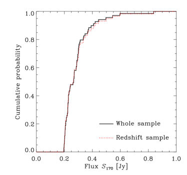
Figure 1: The Kolmogorov–Smirnov test for the whole photometric sample and redshift subsample taken from FIRBACK $170\,\mu$m survey. The solid line shows the cumulative probability distribution of flux densities for the whole sample, while the dotted line depicts that of the redshift sample. The difference is found to be very small.

2.1 Parent sample

The FIRBACK (Far-InfraRed BACKground) survey (Puget et al. 1999; Lagache & Dole 2001; Dole et al. 2001) is one of the deepest surveys performed at $170\;\mu$m by ISO using ISOPHOT (Lemke et al. 1996). It covers $4\;\mbox{deg}^{2}$ on three fields. In this work, we use two of these fields: FIRBACK South Marano field ($0.89\;\mbox{deg}^{2}$) and FIRBACK ELAIS N1 field ($1.87\;\mbox{deg}^{2}$).

The parent sample of FIRBACK is composed of the flux-limited sample of 141 sources with $S_{170}\geq 135\;\mbox{mJy}$ ($3\sigma$ limit). Flux completeness of this parent sample is $75\;\%$, and at flux density $S_{170}\sim 200$ mJy, it becomes $\sim 90$ % (Dole et al. 2001). We use the sources brighter than a flux density of 195 mJy in the following analysis.

2.2 Redshifts and completeness

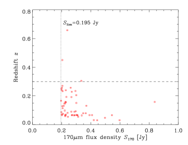
Figure 2: The flux density–redshift distribution of our flux-limited sample. We used a subsample at $z<0.3$ to construct the local luminosity function (LF). The vertical dotted line shows $S_{170}=0.195\;\mbox{Jy}$, and the horizontal dashed line depicts $z=0.3$.

Redshifts are measured for 58 galaxies out of 69 galaxies above the flux density of 195 mJy, i.e., the redshift completeness of the sample used is 84 %. The redshift measurements have been performed by Chapman et al. (2002), Patris et al. (2003), and Dennefeld et al. (2005). Since the redshift measurement becomes more difficult toward the fainter sources, the completeness depends systematically on the flux levels. Thus, we should examine whether the redshift selection distort the flux distribution of the sample.

We performed the Kolmogorov–Smirnov test (e.g., Hoel 1971; Hájek, Šidák, & Sen 1999) to compare the flux-limited sample ($S_{170}\geq 195\leavevmode\nobreak\ \mbox{mJy}$) with the redshift sample (see Figure 1). The maximum difference between the cumulative distribution functions of flux-limited and redshift samples are 0.0377. This shows that we cannot reject the null hypothesis that the two samples are taken from the same parent distribution. Hence, we use the redshift sample as an unbiased subsample of the whole flux-limited sample and simply multiply the inverse of the completeness to obtain the final galaxy density. The distribution of the flux densities and redshifts of the sample is shown in Figure 2.

The redshift completeness of the sample is also tested by $V/V_{\rm max}$ statistics (Schmidt 1968; Rowan-Robinson 1968). Here $V$ is the volume enclosed in a sphere whose radius is the distance of a considered source, and $V_{\rm max}$ is the volume enclosed in a sphere whose radius is the largest distance at which the source can be detected. If the sample is complete, $V/V_{\rm max}$ values of the sample galaxies is expected to distribute uniformely between 0 and 1, with an average $\langle V/V_{\rm max}\rangle=0.5$ and a standard deviation $(12n)^{-1/2}$ ($n$: sample size). For our redshift sample, the mean and standard deviation of the $V/V_{\rm max}$ is $0.66\pm 0.23$, i.e., the sample can be regarded as complete. Moreover, it is larger than 0.5 (but within the uncertainty), suggesting the existence of evolution (see, e.g., Peacock 1999, p.444).

For the estimation of the local LF, we use a subsample of galaxies with $z<0.3$. The size of this ‘low-$z$’ subsample is 55. The mean and median redshift of this low-$z$ sample is 0.12 and 0.09, respectively.

3 Analysis

3.1 $K$-correction

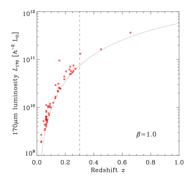
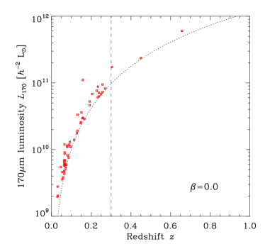
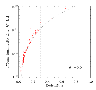
Figure 3: The luminosity–redshift distribution of our redshift sample taken from FIRBACK $170\,\mu$m survey. The luminosity is that at emitted wavelength of 170$\mu$m. The dotted curves represent the limiting luminosities corresponding to the flux density detection limit of 195 mJy at each redshift, including the effect of the $K$-correction. The power-law index of the spectral energy distribution (SED), $\beta$ is 1.0, 0.0, and $-0.5$ from left to right (see the main text). Vertical dashed lines show $z=0.3$, which is used to define our low-$z$ sample.

The monochromatic luminosity at observed frequency $\nu_{\rm obs}$ is obtained by

$${\cal L}_{\nu_{\rm em}}={\cal L}_{(1+z)\nu_{\rm obs}}=\frac{4\pi d_{\rm L}(z)^{2}S_{\nu_{\rm obs}}}{1+z}\;,$$ (1)

where ${\cal L}_{\nu}$ is an energy emitted per unit time at frequency $\nu$, $d_{\rm L}(z)$ is the luminosity distance corresponding to a redshift $z$, and $\nu_{\rm obs}$ and $\nu_{\rm em}$ are observed and emitted frequencies, respectively. In order to estimate the luminosity function at $170\;\mu$m, the $K$-correction is required.

However, the amount of the $K$-correction may be uncertain, because the present sample is observed at one waveband. If we assume a ‘cool’ dust galaxy, the spectral energy distribution (SED) rises toward longer wavelengths, whilst it decreases if we adopt a starburst SED (see e.g., Takeuchi et al. 2001a, b; Lagache, Dole, & Puget 2003). To explore the effect of the $K$-correction, we use a power-law approximation with the form of

$${\cal L}_{\nu}\propto\nu^{\beta}\;.$$ (2)

As for $\beta$, we consider $\beta=1.0$ (starburst galaxies), $0.0$ (intermediate galaxies), and $-0.5$ (cool galaxies). We adopt these values according to the phenomenologically constructed model SEDs of Lagache, Dole, & Puget (2003) (see their Figure 4). Then, the luminosity at the observed frequency $\nu_{\rm obs}$ becomes

$$L_{\nu_{\rm obs}} \equiv \nu_{\rm obs}{\cal L}_{\nu_{\rm obs}}$$ (3)

$$= L_{\nu_{\rm em}}(1+z)^{-(\beta+1)}$$

$$= 4\pi d_{\rm L}(z)^{2}\nu_{\rm obs}S_{\nu_{\rm obs}}(1+z)^{-(\beta+1)}\;.$$

By the same manner, the limiting luminosity of a survey with flux density detection limit $S_{\rm\nu}^{\rm lim}$ depends on the SED via $\beta$,

$$L_{\nu_{\rm obs}}^{\rm lim}=4\pi d_{\rm L}(z)^{2}\nu_{\rm obs}S_{\nu_{\rm obs}}^{\rm lim}(1+z)^{-(\beta+1)}\;.$$ (4)

This is shown with the present sample in Figure 3. The luminosity $L_{170}$ is that at emitted wavelength of $170\;\mu$m, i.e., $L_{\rm em}$ measured at $170\;\mu$m. As we see in the followings, this dependence of the limiting luminosity on $\beta$ potentially affects the estimation of the LF.

3.2 Estimation of the luminosity function

We define the luminosity function as a number density of galaxies whose luminosity lies between a logarithmic interval $[\log L,\log L+d\log L]$:

$$\phi(L)\equiv\frac{dn}{d\log L}\;.$$ (5)

In this work, we denote the luminosity at a certain frequency or wavelength as $L_{\nu}\equiv\nu{\cal L}_{\nu}$.

3.2.1 Parametric estimation

First we performed a parametric maximum likelihood estimation of the LF (Sandage, Tammann, & Yahil 1979). Note that we can do this analysis directly on the data, being independent of the nonparametric result, i.e., this is not a fitting to the nonparametric LF. It is known that the 60-$\mu$m LF is well expressed by a function given by Saunders et al. (1990) which is defined as

$$\phi(L)=\phi_{*}\left(\frac{L}{L_{*}}\right)^{1-\alpha}\exp\left[-\frac{1}{2\sigma^{2}}\log^{2}\left(1+\frac{L}{L_{*}}\right)\right]\;$$ (6)

where $\log^{2}x\equiv(\log x)^{2}$. Since various LFs can be approximated by this functional form, we adopt Equation (6) in this work.

Figure 4: The logarithmic likelihood $\ln{\cal M}$ for the parameter estimation of $L_{*}\;[L_{\odot}]$ and $\sigma$ when we fix $\alpha=1.25$. The outermost contours indicate the 68 % confidence level.

We use Equation (6) for the parametric maximum likelihood estimation. Then the likelihood ${\cal M}$ is expressed as

$${\cal M}(L_{*},\alpha,\sigma|\{L_{i},z_{i}\}_{i=1,\dots,N})=\prod_{i=1}^{N}\frac{\phi(L_{i})}{\int_{\log L_{{\rm min},i}}^{\infty}\phi(L)d\log L}$$

$$=\prod_{i=1}^{N}\frac{\displaystyle\left(\frac{L_{i}}{L_{*}}\right)^{1-\alpha}\exp\left[-\frac{1}{2\sigma^{2}}\log^{2}\left(1+\frac{L_{i}}{L_{*}}\right)\right]}{\displaystyle\int_{\log L_{{\rm min},i}}^{\infty}\left(\frac{L}{L_{*}}\right)^{1-\alpha}\exp\left[-\frac{1}{2\sigma^{2}}\log^{2}\left(1+\frac{L}{L_{*}}\right)\right]d\log L}$$

where

$$L_{{\rm min},i}=L_{\nu_{\rm obs}}^{\rm lim}(z_{i})\;.$$ (8)

Note that, in principle, the parametric estimation procedure is dependent on $\beta$. We can obtain the parameters of the LF by maximizing Equation (3.2.1) with respect to $L_{*}$, $\alpha$, and $\sigma$ (Sandage, Tammann, & Yahil 1979; Saunders et al. 1990; Takeuchi, Yoshikawa, & Ishii 2003).

However, because of the small size of the present sample and relatively narrow range of their luminosity, it is difficult to put a reasonable constraint to the faint-end slope of the LF. Hence instead, as we explain later, we assume a certain value for the faint-end slope $\alpha$.

3.2.2 Nonparametric estimation

We also estimate the LF nonparametrically via an improved version of the $C^{-}$ method of Lynden-Bell (1971), implemented to have the density normalization (Chołoniewski 1987). This method is a kind of maximum likelihood methods insensitive to the density fluctuation. This method and its extension are fully described and carefully examined by Takeuchi, Yoshikawa, & Ishii (2000).

We note that the SED slope $\beta$ also affects the nonparametric estimation of the LF. In the case of $C^{-}$ method, the definition of $C^{-}$ includes $L_{\rm\nu_{\rm obs}}^{\rm lim}$ (see Figure 2 of Takeuchi, Yoshikawa, & Ishii 2000). Thus, it will be important to explore the systematic effect introduced by $K$-correction. The uncertainty (68 % confidence limit) is estimated by the bootstrap resampling (Takeuchi, Yoshikawa, & Ishii 2000). Additionally, we also estimated the LF and uncertainty including the observational measurement errors. For the density normalization, we took into account the source extraction completeness ($\sim 90$ %: Dole et al. 2001) and the redshift measurement (84 %).

4 Results

4.1 Parametric result

We fixed the faint-end slope of the FIRBACK 170-$\mu$m LF to be $1.25$. This is very close to that of the total 60-$\mu$m LF of the IRAS PSC$z$ sample, and the same as that of its ‘cool’ subsample (Takeuchi, Yoshikawa, & Ishii 2003).

We obtained $L_{*}=1.1\times 10^{9}h^{-2}\;[L_{\odot}]$ (with a 68-% confidence range of $3.0\times 10^{8}h^{-2}\mbox{--}2.3\times 10^{9}h^{-2}\;[L_{\odot}]$) and $\sigma=0.41$ (with a 68-% confidence range of $0.35\mbox{--}0.50)$. The likelihood contours are shown in Figure 4. The outermost contours indicate $\Delta\ln{\cal M}\equiv\ln{\cal M}-\ln{\cal M}_{\rm max}=-0.5$, corresponding to the 68-% confidence limit. In Figure 4, we present $\ln{\cal M}$ defined by Equation (3.2.1), as a function of $(L_{*},\sigma)$. These two parameters are rather strongly dependent with one another, and as a result, the contour is elongated along with the diagonal direction in each panel. The density normalization was $\phi_{*}=(1.0\pm 0.4)\times 10^{-1}h^{3}\;[\mbox{Mpc}^{-3}]$. As seen in Figure 4, the result is almost independent of the assumed $\beta$. The result is also found to be quite robust against the value of $\alpha$ in a plausible range of $\alpha=1.1\mbox{--}1.3$.

Takeuchi, Yoshikawa, & Ishii (2003) presented the parameters for the LF of the IRAS PSC$z$ sample. The parameters for the LF of the whole sample are $(\alpha,L_{*},\sigma)=(1.23,4.34\times 10^{8}h^{-2}\;[L_{\odot}],0.724)$. Clearly, the parameters for the 170-$\mu$m sample are different from these values. Particularly, $\sigma$ which determines the steepness of the bright end is significantly smaller than the total IRAS LF. From the above likelihood analysis, $\sigma=0.724$ was rejected with a confidence level of more than 99.9 %, even for the small number of galaxies. That is, the bright end of the present LF declines more steeply than that of the total IRAS LF.

4.2 Nonparametric result

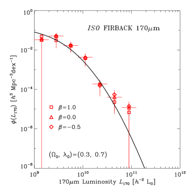
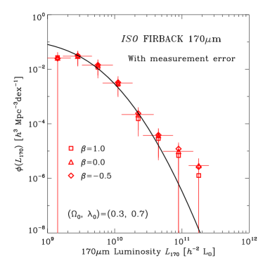
Figure 5: The local luminosity function of ISO FIRBACK 170 $\mu$m galaxy sample. Solid curves show the parametric form estimated from Equation (3.2.1). Symbols represent the $C^{-}$ nonparametric LFs, respectively. Open squares, open triangles, and open diamonds are the LFs adopting $\beta=1.0$, 0.0, and $-0.5$, respectively. Vertical error bars are 68-% confidence ranges. Left panel shows the LF from the original data, while the right panel shows the LF from the data convolved with observational measurement errors. In the left panel, horizontal bars simply represent the bin width (0.3 dex). In the right panel, in contrast, horizontal bars are the convolution of the bin width and the luminosity uncertainty introduced by the photometric error. For visual simplicity, we put horizontal bars only on the case of $\beta=0.0$ in each panel.

Nonparametric LF estimates are presented in Figure 5. Symbols are the LFs obtained by the $C^{-}$-method. Vertical error bars show the 68 % uncertainty, obtained by bootstrap resampling of $10^{4}$ times. Open squares, open triangles, and open diamonds represent $\beta=1.0$, 0.0, and $-0.5$, respectively. Solid lines are the analytic expression of the LF with the parameters we obtained in Section 4.1. We present the numerical tables of our $C^{-}$ LF estimates also in Appendix A.

The left panel is the LF estimates from the original data themselves, while the right panel is the ones from the data convolved with measurement errors. We performed the error convolution procedure assuming a Gaussian distribution for the measurement errors in flux density, with quoted flux density errors as standard deviations for each data. This procedure slightly blurs the LFs horizontally. As a result, we have an additional bin at the highest luminosity, and the 68 % uncertainty levels are broadened. However, the effect is rather small, and the LF estimates are quite robust except for the highest-luminosity unstable bins.

We see that different values for $\beta$ do not affect the result very strongly, but at the highest-luminosity bins, systematic effects are relatively large, a factor of $0.5\mbox{--}0.7\;\mbox{dex}$. In contrast to the large effect of $\beta$ we found in Figure 3, the LF estimates are quite robust against $\beta$. Hence, hereafter, we do not show all the results with respect to $\beta$, but only restrict ourselves to the results with $\beta=0.0$ without loss of generality.

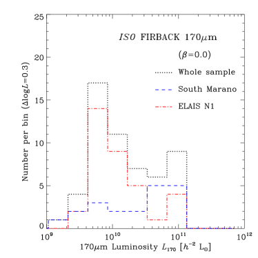
Figure 6: The luminosity distribution of the FIRBACK 170 $\mu$m low-$z$ galaxy sample. The dotted histogram is the luminosity distribution of the whole sample. It has an excess at the highest luminosity bin. The dashed and dot-dashed histograms are those of the subsamples in South Marano field and ELAIS N1 field, respectively.

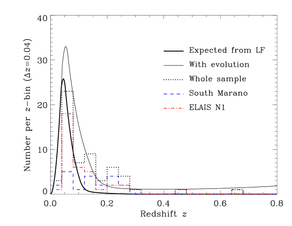
Figure 7: The redshift distribution of our flux-limited sample. The dotted histogram is the distribution of the whole sample, the dashed histogram shows the the subsample in South Marano field, and dot-dashed one presents the subsample in ELAIS N1 field. These histograms present the number of galaxies in each bin ($\Delta z=0.04$). The thick solid curve is the expected distribution of galaxies calculated from the nonparametric local LF (Figure 5). The thin solid curve is the expected distribution for the pure luminosity evolution with $L(z)\propto(1+z)^{5.0}$.

We should note the upward deviation of the $C^{-}$ LF from the analytic result. Although the error bar is large, the $C^{-}$ estimates (open symbols in Figure 5) are about an order of magnitude larger than that of the analytic value. It is worth examining if this deviation is real or merely an artifact of the poor statistics. To see this, we show the luminosity distribution of our present sample in Figure 6. Recall that this sample consists of galaxies only at $z<0.3$. We see an excess at the highest luminosity bin. Examining the subsamples, we also find a similar excess in the ELAIS N1 field. We, however, also see that the sample in South Marano field is interesting: the galaxies in this subsample are biased toward higher luminosities. The superposition of these effects makes the brightest end of the nonparametric LF deviated from the analytic one.

Why does the analytic maximum likelihood not reflect this sample property? We see that, though there is an excess at $L_{170}\simeq 10^{11}h\;L_{\odot}$, the majority of the sample is located around $10^{10}h\;L_{\odot}$ (the peak in Figure 6). Hence, the parameter estimation is practically controlled by the sample around $L_{*}$, and the bright galaxies could hardly give a strong effect to the final estimation. In addition, the peak is dominated by the sample from ELAIS N1 field, and the peculiar luminosity distribution of South Marano field affected the result little. We, hence, should not overly rely on the analytic result and parameters, but rather we should use the nonparametric $C^{-}$ LF directly. These are small sample effects, and we should wait for the larger sample to clarify the detailed shape of the LF.

We show the redshift distribution of the present sample in Figure 7. The histograms show the distribution of the present data. The thick solid curve is the expected redshift distribution of galaxies calculated from the nonparametric local LF we have obtained. This is calculated as follows

$$\frac{dN}{dz}=\Omega_{\rm survey}\int_{\log L_{\rm min}(z)}^{\infty}\phi(L_{170})\frac{d^{2}V}{d\Omega dz}d\log L_{170}\;,$$ (9)

where $L_{\rm min}(z)$ is the minimum detectable luminosity $L_{{\nu}_{\rm obs}}^{\rm lim}(z)$ [see, Eq. (8)], and

$$\frac{d^{2}V}{d\Omega dz}=\frac{c}{H_{0}}\frac{d_{\rm L}(z)^{2}}{(1+z)^{2}\sqrt{\Omega_{0}(1+z)^{3}+\lambda_{0}}}$$ (10)

for the flat lambda-dominated universe (see, e.g., Peebles 1993), i.e., $(d^{2}V/d\Omega dz)dz$ is the comoving volume between $[z,z+dz]$ per unit solid angle. This curve is calculated to apply to the solid angle of the survey area by multiplying $\Omega_{\rm survey}=8.4\times 10^{-4}\;\mbox{sr}$. We used the nonparametric LF for Figure 7 because the exact shape of the bright end of the LF is crucial to examine the tail of the redshift distribution of the source toward higher $z$, and as already discussed, the analytic function underproduces galaxies with $L_{170}\ga 3\times 10^{10}\;L_{\odot}$. We find a density excess at $z\simeq 0.2$ in Figure 7. However, apart from the bump, both fields have long tails toward higher redshifts than expected from the local LF. It may suggest the existence of galaxy evolution. We explore the effect of the evolution in Section 5.2

5 Discussion

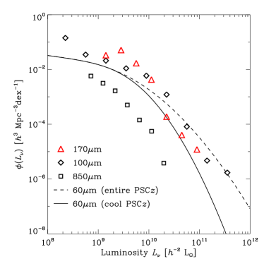
Figure 8: Comparison of the 170-$\mu$m LF with those at other FIR wavelengths. Open triangles are our 170-$\mu$m LF ($\beta=0.0$), open diamonds represent the 100-$\mu$m LF of Soifer & Neugebauer (1991), and open squares represent the 850-$\mu$m LF of Dunne et al. (2000). The dashed curve is the analytic form of the 60-$\mu$m LF of the IRAS PSC$z$ entire sample, and the solid curve is the LF of the cool subsample of the IRAS PSC$z$ galaxies (Takeuchi, Yoshikawa, & Ishii 2003). The 850-$\mu$m LF is horizontally shifted by a factor of 100 for display purposes.

5.1 Shape of the $170\;\mu$m LF

The overall shape of the 170-$\mu$m LF of the FIRBACK galaxies is different from the IRAS 60-$\mu$m LF. As we discussed in Section 4.1, the parameters of the analytic LF suggest a steeper slope for the bright end of the LF. Although the nonparametric LF revealed that the brightest part of the LF is significantly higher than that of the analytic LF, the 170-$\mu$m LF decreases more rapidly from the knee of the LF to the bright end than the IRAS 60-$\mu$m LF. Here we compare the 170-$\mu$m LF with other FIR LFs obtained to date.

Takeuchi, Yoshikawa, & Ishii (2003) divided the IRAS sample into two categories, warm and cool subsamples, using the flux density ratio criterion of $S_{100}/S_{60}=2.1$. The parameters of the cool galaxies are $(\alpha,L_{*},\sigma)=(1.25,9.55\times 10^{9}h^{-2}\;[L_{\odot}],0.50)$. The $\alpha$ is almost the same as that of the total IRAS LF within the quoted error, but $L_{*}$ and $\sigma$ are much closer to those of our present LF. The resemblance of our LF to the LF of cool IRAS galaxies may be reasonable, since the present sample is selected at $170\;\mu$m band, where we can detect cooler galaxies more effectively than $60\;\mu$m. Soifer & Neugebauer (1991) derived a LF at $100\;\mu$m from IRAS galaxy sample. Their 100-$\mu$m LF has a bright end slightly steeper than 60-$\mu$m LF does, but the slope is still flatter than our LF. Dunne et al. (2000) constructed a LF at $850\;\mu$m based on 60-$\mu$m selected IRAS galaxy sample. Although the dynamic range is small, the overall shape of their 850-$\mu$m LF is similar to our LF. Actually, Dunne et al. (2000) fitted their LF with the Schechter function which has a very steep decline at the bright end (Schechter 1976).

In summary, the 170-$\mu$m LF has a shape similar to those of galaxy sample with cool dust emission. It is also interesting to note that the 170-$\mu$m LF has the highest normalization among known FIR LFs. We summarize the comparison in Figure 8. However, we must keep in mind the large uncertainty of the estimates, and further observational exploration is definitely required.

5.2 Evolution

5.2.1 Pure luminosity evolution assumption

Most of the galaxies in our redshift sample are at $z<0.3$. Hence, we should estimate the evolution of the LF under a certain assumption. We adopt a pure luminosity evolution (PLE). Recent Spitzer observations indicated that the actual evolution of IR galaxies is described as a strong evolution in luminosity, with a slight evolution in density (e.g., Pérez-González et al. 2005; Le Floc’h et al. 2005), while their studies are based on the Spitzer $24\;\mu$m band. Hence, the PLE is not a bad choice as a first approximation.

Adopting the PLE, the strength of the evolution can be estimated via a radial density distribution of galaxies (Saunders et al. 1990). In the case of the PLE, the LF at $z$ is expressed by the evolution strength $f(z)$ as

$$\phi(L,z)=\phi_{0}\left[\frac{L}{f(z)}\right]\;,$$ (11)

where $\phi_{0}(L)$ is the local functional form of the LF. The PLE assumes that this form remains unchanged and only shifts along the luminosity axis. To define $\phi_{0}(L_{170})$, we examined the 170-$\mu$m LF for a sample at $z<0.15$ (38 galaxies). Though the uncertainty is large, we did not observe a significant change of the LF in its shape, i.e., the PLE assumption might be approximately valid. Hence, we can use the shape of the LF of the sample with $z<0.3$ as $\phi_{0}(L_{170})$. For simplicity, we consider a power-law form for $f(z)$:

$$f(z)=(1+z)^{Q}\;,$$ (12)

but this form is supported by recent Spitzer observations at a wide redshift range of $z=0\mbox{--}1$ (Pérez-González et al. 2005; Le Floc’h et al. 2005).

5.2.2 Estimation of evolution via radial density

Assuming that the LF is separable for $L$ and $z$ as $\phi(L,z)=n(z)p(L)$, the likelihood is written as

$${\cal M}(Q|\{L_{i},z_{i}\}_{i=1,\dots,N})=\prod_{i=1}^{N}\frac{\phi(L_{i},z_{i})}{\displaystyle\int_{z_{\rm min}}^{z_{{\rm max},i}}\phi(L_{i},z)\frac{d^{2}V}{d\Omega dz}dz}$$ (13)

where $N$ is the total sample size, $z_{\rm min}$ is the lowest redshift which we used in the analysis, $z_{{\rm max},i}$ is the maximum redshift to which $i$th galaxy can be detected, and $(d^{2}V/d\Omega dz)dz$ is again the differential comoving volume [Eq. (10)].

By maximizing Equation (13) with respect to $Q$, we can have a maximum likelihood estimate. We performed this procedure with the nonparametric LF, because as we already mentioned, the analytic form underestimates the bright end of the LF, and it would lead to a serious overestimation of the evolution strength. We obtained $Q=5.0^{+2.5}_{-0.5}$. The expected redshift distribution with this evolution is obtained by a similar manner to Equation (9) as

$$\frac{dN}{dz}=\Omega_{\rm survey}\int_{\log L_{\rm min}(z)}^{\infty}\phi_{0}\left[\frac{L_{170}}{(1+z)^{Q}}\right]\frac{d^{2}V}{d\Omega dz}d\log L_{170}\;,$$ (14)

and shown in Figure 7 (the thin solid line). The agreement with the data and the expected value is much improved.

Although the uncertainty is very large because of the limited sample size, this is similar to the value obtained by recent Spitzer 24-$\mu$m observations, $Q\simeq 4$ (Pérez-González et al. 2005; Le Floc’h et al. 2005). These authors also found a weak evolution in the galaxy number density, but for the present sample, it is impossible to explore this effect. If confirmed, the similarity between the strength of the galaxy evolution in the MIR (12-$\mu$m in the rest frame) and FIR will provide us an important clue to the physics of dusty star formation in galaxies.

5.3 FIR luminosity density and obscured star formation density in the Local Universe

5.3.1 The local 170-$\mu$m and total IR luminosity density

Figure 9: The MIR and FIR luminosity densities in the Local Universe. The filled square represent the 170-$\mu$m luminosity density, $\rho_{L}(170\mu\mbox{m})$, obtained by a direct integration of our LF. The vertical error bar shows the total uncertainty related to the LF. The horizontal bar represents the redshift range of our local sample ($0\leq z<0.3)$. The filled triangle is the corrected $\rho_{L}(170\mu\mbox{m})$ by assuming a pure luminosity evolution $L(z)\propto(1+z)^{5}$. Open squares present the luminosity densities at 12, 25, 60, 100, and $850\;\mu$m calculated based on the literatures (see text).

The luminosity density in a cosmic volume provides various information of the energy distribution in the Universe. Especially, comparison between the radiative energy directly emitted from stars and that re-emitted from dust is one of the key quantities to understand the fraction of hidden star formation. In this subsection, we discuss the local luminosity density at $170\;\mu$m, $\rho_{L}(170\mu\mbox{m})\;[L_{\odot}\mbox{Mpc}^{-3}]$ and consider the integrated SED of the Local Universe.

In principle, it is straightforward to obtain $\rho_{L}(170\mu\mbox{m})$ from the LF: we simply integrate the first-order moment of the LF, $L_{170}\phi(L_{170})$, over the whole possible range of luminosity. Since the luminosity range of the 170-$\mu$m LF is limited to $10^{9}\mbox{--}10^{12}\;L_{\odot}$, we extrapolated the faint end without observed data. We have done it by using the analytic form (Eq. 6) with various $\alpha$. However, as far as $\alpha<2.0$, the integration of $L_{170}\phi(L_{170})$ converges and the faint end does not contribute to the total integration significantly. For the infrared (IR) galaxies, previous studies suggest $\alpha<2.0$ (e.g., Saunders et al. 1990; Takeuchi, Yoshikawa, & Ishii 2003, and references therein), and the $\rho_{L}(170\mu\mbox{m})$ is little affected by $\alpha$. By the same reason, the lower and upper bounds of the integration do not affect the result. We chose $10^{7}h^{-2}[L_{\odot}]$ as the lowest luminosity, and use the highest luminosity bin as the upper bound. Thus, we obtained $\rho_{L}(170\mu\mbox{m})=(1.1^{+0.5}_{-0.4})\times 10^{8}h[L_{\odot}\mbox{Mpc}^{-3}]$. The final uncertainty of $\rho_{L}(170\mu\mbox{m})$ is dominated by the statistical uncertainty of the nonparametric LF in each bin.

We, however, must recall that the present FIRBACK sample is not exactly ‘local’, i.e., it consists of galaxies $0\leq z<0.3$. As seen in the previous subsection, it may be plausible that this result is affected by the strong galaxy evolution. If we adopt a PLE $L(z)\propto(1+z)^{5.0}$, $\rho_{L}(170\mu\mbox{m})$ should be enhanced by a factor of 2.1 on average in this redshift range. By correcting the evolution, we have $\rho_{L}(170\mu\mbox{m})=5.20\times 10^{7}h[L_{\odot}\mbox{Mpc}^{-3}]$.

We plot the result in Figure 9. The filled square represents the 170-$\mu$m luminosity density obtained by a direct integration of our LF. The horizontal bar indicates that the redshift range of our low-$z$ sample is $0\leq z<0.3$. The filled triangle shows the evolution-corrected value. Then, we consider the SED of the luminosity density in the Local Universe. We do similar exercises to calculate $\rho_{L}(\lambda)$ at various IR wavelengths. At MIR, Fang et al. (1998) and Shupe et al. (1998) provided the LFs at IRAS 12 and $25\;mu$m bands, respectively. Fang et al. (1998) tabulated their nonparametric LF at approximately the same luminosity range as we adopt in this work ($10^{7}L_{\odot}\mbox{--}10^{12}L_{\odot}$). We simply summed it up with multiplying the luminosity and obtained $\rho_{L}(12\mu\mbox{m})=1.79\times 10^{7}h\;[L_{\odot}\mbox{Mpc}^{-1}]$. Shupe et al. (1998) provided an analytic fit for their 25-$\mu$m LF. By their analytic function, we got $\rho_{L}(25\mu\mbox{m})=1.42\times 10^{7}h\;[L_{\odot}\mbox{Mpc}^{-1}]$. At $60\;\mu$m, from Takeuchi, Yoshikawa, & Ishii (2003), we obtained $\rho_{L}(60\mu\mbox{m})=4.08\times 10^{7}h\;[L_{\odot}\mbox{Mpc}^{-1}]$. Soifer & Neugebauer (1991) presented the LFs at all the IRAS bands. Using their 100-$\mu$m nonparametric LF, we re-calculated the luminosity density to obtain $\rho_{L}(100\mu\mbox{m})=8.25\times 10^{7}h\;[L_{\odot}\mbox{Mpc}^{-1}]$. Lastly, we used the Schechter function fit provided by Dunne et al. (2000) to have $\rho_{L}(850\mu\mbox{m})$. Since their faint-end slope is very steep ($\alpha=2.12$), the integration is dependent on the adopted lowest luminosity in this case. We coherently integrated the Schechter function in the same range as the other bands. We found $\rho_{L}(850\mu\mbox{m})=1.00\times 10^{5}h\;[L_{\odot}\mbox{Mpc}^{-1}]$.

We plot these luminosity densities in Figure 9 (open squares). The overall peak of the SED of the luminosity density seems to lie at $\lambda\ga 100\;\mu$m. Further, if the suggested strong evolution is true, the local SED peak is restricted to be at $100\ga\lambda\ga 170\;\mu$m. Even though the evolution effect significantly reduces the local $\rho_{L}(170\mu\mbox{m})$ value, it still considerably contributes to the total FIR luminosity density.

Table 1: The SED of the luminosity density in the Local Universe.

$\lambda$	$\rho_{L}(\lambda)$	$\rho_{L}(\lambda)/\rho_{L}(170\,\mu\mbox{m})$
$[\mu\mbox{m}]$	$h\;[L_{\odot}\mbox{Mpc}^{-3}]$
12	$1.79\times 10^{7}$	$3.3\times 10^{-1}$
25	$1.42\times 10^{7}$	$2.6\times 10^{-1}$
60	$4.08\times 10^{7}$	$7.5\times 10^{-1}$
100	$8.25\times 10^{7}$	$1.5$
170	$5.20\times 10^{7}$ a	$1$
850	$9.45\times 10^{4}$ b	$1.7\times 10^{-3}$

• The effect of the evolution is corrected assuming a pure luminosity evolution with $L(z)\propto(1+z)^{Q}$ ($Q=5.0$).

• This value is calculated by integrating a Schechter function presented by Dunne et al. (2000), over the luminosity range of $L_{850}=10^{7}L_{\odot}\mbox{--}10^{13}L_{\odot}$.

To have a crude estimate of the total IR luminosity density (we call it $\rho_{L}(\mbox{dust})$), we logarithmically interpolate and extrapolate between the SED data points in units of $[\mbox{erg\,s}^{-1},\mbox{Hz}^{-1}\mbox{Mpc}^{-3}]$, and integrate it over the range of $8\mbox{--}1000\;\mu$m to match the conventional definition of the total IR (TIR) luminosity (see, e.g., Dale et al. 2001; Dale & Helou 2002; Takeuchi et al. 2005). If we do not assume the evolution, we have $\rho_{L}(\mbox{dust})=1.4\times 10^{8}h\;[L_{\odot}\mbox{Mpc}^{-3}]$, and with the evolution, $\rho_{L}(\mbox{dust})=1.1\times 10^{8}h\;[L_{\odot}\mbox{Mpc}^{-3}]$. Takeuchi, Buat, & Burgarella (2005) estimated the $\rho_{L}(\mbox{dust})$ under the assumption of a constant ratio of $\rho_{L}(\mbox{dust})/\rho_{L}(60\mu\mbox{m})=2.5$ (see, e.g., Takeuchi et al. 2005). They found $\rho_{L}(\mbox{dust})=1.02\times 10^{8}h\;[L_{\odot}\mbox{Mpc}^{-3}]$. Our $\rho_{L}(\mbox{dust})$ values are in a very good agreement with that, especially for the case with evolution.

For the interpretation of the IR luminosity density, it should be worth mentioning that there is a possibly high contamination by active galactic nuclei (AGN) at 12 and 24 $\mu$m. However, by integrating over the energy density from these wevelengths, we find that the contribution from 12 and 24 $\mu$m bands to $\rho_{L}(\mbox{dust})$ is less than 10 %. Hence, if all the energy from 12 and 24 $\mu$m were from the AGN, the effect of AGNs would not change the physical interpretation of $\rho_{L}(\mbox{dust})$ significantly.

5.3.2 The obscured star formation density in the Local Universe

The ratio between the energy from young stars directly observed at UV and that reprocessed by dust and observed at IR in the cosmic history has long been a matter of debate. Before closing the discussion, we consider the star formation rate density in the Local Universe obscured by dust. We use the value with evolutionary correction in the rest of this work. To get values without this evolutionary correction, we may simply substitute the former value for $\rho_{L}(\mbox{dust})$.

For the conversion from $\rho_{L}(\mbox{dust})$ to the cosmic star formation rate (SFR) density related to dust, $\rho_{\rm SFR}(\mbox{dust})$, we can use several methods. Kennicutt (1998) presented a famous formula between the SFR and the dust luminosity, $L_{\rm dust}\;[L_{\odot}]$,

$$\mbox{SFR}\;[M_{\odot}\,\mbox{yr}^{-1}]=1.72\times 10^{-10}\;L_{\rm dust}\;[L_{\odot}]\;,$$ (15)

which is valid for starburst galaxies with a burst younger than $10^{8}$ yr. Adopting this formula to $\rho_{L}(\mbox{dust})$, we obtained $\rho_{\rm SFR}(\mbox{dust})=1.89\,h\times 10^{-2}\;[M_{\odot}\,\mbox{yr}^{-1}\mbox{Mpc}^{-3}]$. However, as mentioned by Kennicutt (1998) himself, this formula is not valid for more quiescent, normal galaxies. Since our SED of the Local Universe is similar to a kind of cool galaxies, we should carefully treat the effect of the heating radiation from old stars. Hirashita, Buat, & Inoue (2003) found that about 40 % of the dust heating in the nearby galaxies comes from stars older than $10^{8}$ yr. If we apply the correction of old stellar population to Equation (15), we obtain $\rho_{\rm SFR}(\mbox{dust})=1.14\,h\times 10^{-2}\;[M_{\odot}\,\mbox{yr}^{-1}\mbox{Mpc}^{-3}]$. Bell (2003) also presented a similar correction factor ($0.32\pm 0.16$ for galaxies with $L_{\rm dust}\leq 10^{11}L_{\odot}$ and $0.09\pm 0.05$ for those with $L_{\rm dust}>10^{11}L_{\odot}$) for the contribution of old stars. Based on a more theoretical point of view, Takeuchi, Buat, & Burgarella (2005) also obtained an appropriate formula including the correction, which can be written as

$$\mbox{SFR}\;[M_{\odot}\,\mbox{yr}^{-1}]=1.07\times 10^{-10}\;L_{\rm dust}\;[L_{\odot}]\;.$$ (16)

Adopting Equation (16), we obtain $\rho_{\rm SFR}(\mbox{dust})=1.17\,h\times 10^{-2}\;[M_{\odot}\,\mbox{yr}^{-1}\mbox{Mpc}^{-3}]$, very close to the above. The obtained $\rho_{\rm SFR}(\mbox{dust})$ is slightly larger than the local SFR density estimated from direct FUV radiation (without dust attenuation correction), $\rho_{\rm SFR}(\mbox{FUV})=8.3\times 10^{-3}[M_{\odot}\,\mbox{yr}^{-1}\mbox{Mpc}^{-3}]$ (Takeuchi, Buat, & Burgarella 2005; see also Schiminovich et al. 2005). Hence, 58.5 % of the star formation is obscured by dust in the Local Universe. This is in very good agreement with that of Takeuchi, Buat, & Burgarella (2005), but since we reached this conclusion from the measured dust SED of the Local Universe, we could put a firmer basis on their conclusion by this work. These results may be the first direct estimate of the dust luminosity in the Local Universe, and should be tested by forthcoming large area survey in the FIR by e.g., ASTRO-F.

6 Conclusion

We analyzed the FIRBACK $170\;\mu$m galaxy sample to obtain the local luminosity function (LF) of galaxies. We constructed a flux-limited sample with $S_{170}\geq 0.195\;\mbox{Jy}$ and $z<0.3$ from the survey, which consists of 55 galaxies.

The overall shape of the 170-$\mu$m LF is quite different from that of the total 60-$\mu$m LF (Takeuchi, Yoshikawa, & Ishii 2003): the bright end of the LF declines more steeply than that of the 60-$\mu$m LF. This behavior is quantitatively similar to the LF of the cool subsample of the IRAS PSC$z$ galaxies. The bright end is also similar to that of the submillimeter LF of Dunne et al. (2000).

We also estimated the strength of the evolution of the LF by assuming the pure luminosity evolution $L(z)\propto(1+z)^{Q}$. We obtained $Q=5.0^{+2.5}_{-0.5}$ which is similar to the value obtained by recent Spitzer observations (Pérez-González et al. 2005; Le Floc’h et al. 2005), in spite of the limited sample size.

Then, integrating over the 170-$\mu$m LF, we obtained the local luminosity density at $170\;\mu$m, $\rho_{L}(170\mu\mbox{m})\;[L_{\odot}\mbox{Mpc}^{-3}]$. If we assume the above strong luminosity evolution $L(z)\propto(1+z)^{5}$, the value is $5.2\times 10^{7}h\;[L_{\odot}\mbox{Mpc}^{-3}]$, which is a considerable contribution to the local FIR luminosity density.

By summing up the other MIR/FIR data, we obtained the total dust luminosity density in the Local Universe. We obtained $\rho_{L}(\mbox{dust})=1.1\times 10^{8}h\;[L_{\odot}\mbox{Mpc}^{-3}]$ without the evolution correction, and $\rho_{L}(\mbox{dust})=1.1\times 10^{8}h\;[L_{\odot}\mbox{Mpc}^{-3}]$ with correction.

Lastly, based on $\rho_{L}(\mbox{dust})$, we estimated the cosmic star formation rate (SFR) density hidden by dust in the Local Universe. We took into account the dust emission heated by old stellar population, and obtained $\rho_{\rm SFR}(\mbox{dust})\simeq 1.1\mbox{--}1.2\,h\times 10^{-2}\;[M_{\odot}\,\mbox{yr}^{-1}\mbox{Mpc}^{-3}]$. Comparing with the SFR density estimated form FUV observation (Takeuchi, Buat, & Burgarella 2005), we found that 58.5 % of the star formation is obscured by dust in the Local Universe.

It will be important to examine our local LF by a large area survey of the Local Universe. The ASTRO-F project promises to provide a local large sample of FIR galaxies at $\simeq 50\mbox{--}170\;\mu$m. For the evolutionary status of the FIR galaxies, the FIR data of Spitzer will be very important to examine the present result.

Appendix A Tables of the nonparametric luminosity function

Table 2: The 170-$\mu$m luminosity function with $\beta=1.0$, estimated with Lynden-Bell’s $C^{-}$ method.

${\log L_{170}}^{\mathrm{a}}$	$\phi(L_{170})$	$\phi(L_{170})^{\rm upper}$	$\phi(L_{170})^{\rm lower}$
	$h^{3}\;[\mbox{Mpc}^{-3}\mbox{dex}^{-1}]$	$h^{3}\;[\mbox{Mpc}^{-3}\mbox{dex}^{-1}]$	$h^{3}\;[\mbox{Mpc}^{-3}\mbox{dex}^{-1}]$
9.15	$4.89\times 10^{-2}$	$6.20\times 10^{-2}$	$0.00\times 10^{+0}$
9.45	$3.10\times 10^{-2}$	$4.96\times 10^{-2}$	$1.24\times 10^{-2}$
9.75	$1.73\times 10^{-2}$	$2.63\times 10^{-2}$	$7.70\times 10^{-3}$
10.05	$3.81\times 10^{-3}$	$5.99\times 10^{-3}$	$1.43\times 10^{-3}$
10.35	$1.81\times 10^{-4}$	$3.00\times 10^{-4}$	$5.95\times 10^{-5}$
10.65	$2.29\times 10^{-5}$	$3.85\times 10^{-5}$	$5.54\times 10^{-6}$
10.95	$6.87\times 10^{-6}$	$1.17\times 10^{-5}$	$0.00\times 10^{+0}$

• Units of $L_{170}$ is $h^{-2}\;[\;L_{\odot}]$, and the bin width is $0.3\;\mbox{dex}$. Tabulated log luminosities represent the bin center.

Table 3: Same as Table 2 but for $\beta=0.0$.

$\log L_{170}$	$\phi(L_{170})$	$\phi(L_{170})^{\rm upper}$	$\phi(L_{170})^{\rm lower}$
	$h^{3}\;[\mbox{Mpc}^{-3}\mbox{dex}^{-1}]$	$h^{3}\;[\mbox{Mpc}^{-3}\mbox{dex}^{-1}]$	$h^{3}\;[\mbox{Mpc}^{-3}\mbox{dex}^{-1}]$
9.15	$3.33\times 10^{-2}$	$4.65\times 10^{-2}$	$0.00\times 10^{+0}$
9.45	$5.12\times 10^{-2}$	$7.17\times 10^{-2}$	$3.10\times 10^{-2}$
9.75	$1.69\times 10^{-2}$	$2.56\times 10^{-2}$	$7.42\times 10^{-3}$
10.05	$4.29\times 10^{-3}$	$6.80\times 10^{-3}$	$1.69\times 10^{-3}$
10.35	$1.89\times 10^{-4}$	$3.16\times 10^{-4}$	$5.95\times 10^{-5}$
10.65	$4.04\times 10^{-5}$	$7.00\times 10^{-5}$	$7.20\times 10^{-6}$
10.95	$1.20\times 10^{-5}$	$2.01\times 10^{-5}$	$0.00\times 10^{+0}$

Table 4: Same as Table 2 but for $\beta=-0.5$.

$\log L_{170}$	$\phi(L_{170})$	$\phi(L_{170})^{\rm upper}$	$\phi(L_{170})^{\rm lower}$
	$h^{3}\;[\mbox{Mpc}^{-3}\mbox{dex}^{-1}]$	$h^{3}\;[\mbox{Mpc}^{-3}\mbox{dex}^{-1}]$	$h^{3}\;[\mbox{Mpc}^{-3}\mbox{dex}^{-1}]$
9.15	$3.37\times 10^{-2}$	$4.65\times 10^{-2}$	$0.00\times 10^{+0}$
9.45	$5.14\times 10^{-2}$	$7.21\times 10^{-2}$	$3.10\times 10^{-2}$
9.75	$1.67\times 10^{-2}$	$2.54\times 10^{-2}$	$7.45\times 10^{-3}$
10.05	$4.12\times 10^{-3}$	$6.57\times 10^{-3}$	$1.53\times 10^{-3}$
10.35	$1.56\times 10^{-4}$	$2.63\times 10^{-4}$	$4.51\times 10^{-5}$
10.65	$5.45\times 10^{-5}$	$9.37\times 10^{-5}$	$1.11\times 10^{-5}$
10.95	$1.40\times 10^{-5}$	$2.40\times 10^{-5}$	$0.00\times 10^{+0}$

In this section, we present numerical tables of the nonparametric luminosity function (LF) of the FIRBACK $170\;\mu$m galaxy sample obtained with the $C^{-}$-method. We only tabulate the LF directly estimated from the original data, and the flux measurement errors are not included in these LFs.

Appendix B Comparison between the $1/V_{\rm max}$- and $C^{-}$-luminosity functions

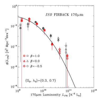
Figure 10: Comparison of the luminosity functions of our ISO 170 $\mu$m galaxy sample by $1/V_{\rm max}$ and $C^{-}$ estimators. Thick and thin symbols represent the $C^{-}$ nonparametric LFs, respectively. The signification’s of the symbols are the same as Figure 5 The symbols for $1/V_{\rm max}$ estimates are shifted with 0.05 dex for th purpose of visual clarity.

In this section, we examine the problem of the classical $1/V_{\rm max}$ estimator (Schmidt 1968; Eales 1993). Comparison of the luminosity functions of our ISO 170 $\mu$m galaxy sample by $1/V_{\rm max}$ and $C^{-}$ estimators is shown in Figure 10. In Figure 10, the $1/V_{\rm max}$ LFs are shifted to the left with $0.05\;{\rm dex}$ to make them easy to see, but the actual bin centers are exactly the same as those of $C^{-}$ LFs. It is impressive that there is a large difference between the $1/V_{\rm max}$ and $C^{-}$ LFs. At the fainter side, these two LFs are consistent with one another within the error bars, though the faint end of the $1/V_{\rm max}$ LFs tend to be slightly underestimated. In contrast, the bright end is completely different: $1/V_{\rm max}$ method gives much flatter LFs than $C^{-}$ method. We should recall that the parametric method and the $C^{-}$ method are both insensitive to density fluctuation, while $1/V_{\rm max}$ method is unbiased only for the spatially homogeneous sample, as extensively examined by Takeuchi et al. (2000). Then, the most plausible explanation of this discrepancy may be due to the existence of a density enhancement, corresponding to the luminosity $L_{170}\ga 3\times 10^{10}\;L_{\odot}$.

To understand more clearly, we recall the redshift distribution of the present sample (Figure 7). The distribution of ELAIS N1 galaxies is not very far from that expected by the LF, while that of South Marano galaxies are very different. Reflecting the luminosity distribution of this field, which is heavily inclined to luminous galaxies, the distribution has no apparent peak, but has a widely spread shape toward redshifts up to $\sim 0.3$. This heavy high-$z$ tail is superposed to the tail of the ELAIS N1 field makes a significant bump at $z\simeq 0.2$. Since the $1/V_{\rm max}$ method assumes a spatially homogeneous source distribution, this excess is too much exaggerated through the number density estimation, and results in the overestimation of the corresponding luminosity bins.

References

- Bell (2003) Bell, E. F. 2003, ApJ, 586, 794
- Chapman et al. (2002) Chapman, S. C., Smail, I., Ivison, R. J., et al. 2002, ApJ, 573, 66
- Chołoniewski (1986) Chołoniewski, J. 1986, MNRAS, 223, 1
- Chołoniewski (1987) Chołoniewski, J. 1987, MNRAS, 226, 273
- Dale et al. (2001) Dale, D. A., Helou, G., Contursi, A.,Silbermann, N. A., Kolhatkar, S. 2001, ApJ, 549, 215
- Dale & Helou (2002) Dale, D. A., & Helou, G. 2002, ApJ, 576, 159
- Dennefeld et al. (2005) Dennefeld, M., Lagache, G., Mei, S., et al. 2005, A&A, 440, 5
- Dole et al. (2001) Dole, H., Gispert, R., Lagache, G., et al. 2001, A&A, 372, 364
- Dunne et al. (2000) Dunne, L., Eales, S., Edmunds, M., et al. 2000, MNRAS, 315, 115
- Eales (1993) Eales, S. 1993, ApJ, 404, 51
- Efstathiou et al. (1988) Efstathiou, G., Ellis, R. S., & Peterson, B. A. 1988, MNRAS, 232, 431
- Fang et al. (1998) Fang, F., Shupe, D. L., Xu, C., & Hacking, P. B. 1998, ApJ, 500, 693
- Franceschini et al. (1998) Franceschini, A., Andreani, P., & Danese, L. 1998, MNRAS, 296, 709
- Frayer et al. (2005) Frayer, D. T., Fadda, D., Yan, L., et al. 2005, AJ, in press (astro-ph/0509649)
- Gispert et al. (2000) Gispert, R., Lagache, G., & Puget, J. L. 2000, A&A, 360, 1
- Hájek, Šidák, & Sen (1999) Hájek, J., Šidák, Z., & Sen, P. K. 1999, Theory of Rank Tests, 2nd ed. (San Diego: Academic Press)
- Hauser & Dwek (2001) Hauser, M. G., & Dwek, E. 2001, ARA&A, 39, 249
- Hirashita, Buat, & Inoue (2003) Hirashita, H., Buat, V., & Inoue, A. K. 2003, A&A, 410, 83
- Hoel (1971) Hoel, P. G., 1978, Introduction to Mathematical Statistics, 4th ed. (New York: John Wiley & Sons), pp.318–322
- Isobe & Feigelson (1992) Isobe, T., & Feigelson, E. D., 1992, ApJS, 79, 197
- Kennicutt (1998) Kennicutt, R. C. 1998, ARA&A, 36, 189
- Koranyi & Strauss (1997) Koranyi, D. M., & Strauss, M. A., 1997, ApJ, 477, 36
- Lagache & Dole (2001) Lagache, G., & Dole, H. 2001, A&A, 372, 702
- Lagache, Dole, & Puget (2003) Lagache, G., Dole, H., & Puget, J.-L., 2003, MNRAS, 338, 555
- Lagache, Dole, & Puget (2005) Lagache, G., Dole, H., & Puget, J.-L., 2005, ARA&A, 43, 727
- Lawrence et al. (1986) Lawrence, A., Walker, D., Rowan-Robinson, M.,et al. 1986, MNRAS, 219, 687
- Le Floc’h et al. (2005) Le Floc’h, E., Papovich, C., Dole, H., et al., 2005, ApJ, 632, 169
- Lemke et al. (1996) Lemke, D., Klaas, U., Abolins, J., et al. 1996, A&A, 315, L64
- Lynden-Bell (1971) Lynden-Bell, D. 1971, MNRAS, 155, 95
- Oyabu et al. (2005) Oyabu, S., Yun, M. S., Murayama, T., et al. 2005, AJ, 130, 2019
- Patris et al. (2003) Patris, J., Dennefeld, M., Lagache, G., & Dole, H. 2003, A&A, 412, 349
- Peacock (1999) Peacock, J. A. 1999, Cosmological Physics (Cambridge: Cambridge University Press), p.444
- Peebles (1993) Peebles, P. J. E. 1993, Principles of Physical Cosmology (Princeton: Princeton University Press), pp.314–317
- Pérez-González et al. (2005) Pérez-González, P. G., Rieke, G. H., Egami, E., et al. 2005, ApJ, 630, 82
- Puget et al. (1999) Puget, J. L., et al. 1999, A&A, 345, 29
- Rieke & Lebofsky (1986) Rieke, G. H., & Lebofsky M. J. 1986, ApJ, 304, 326
- Rowan-Robinson (1968) Rowan-Robinson, M. 1968, MNRAS, 138, 445
- Rowan-Robinson et al. (1987) Rowan-Robinson, M., Helou, G., & Walker, D. 1987, MNRAS, 227, 589
- Rush et al. (1993) Rush, B., Malkan, M. A., & Spinoglio, L. 1993, ApJS, 89, 1
- Sandage, Tammann, & Yahil (1979) Sandage, A., Tammann, G. A., & Yahil, A., 1979, ApJ, 232, 352
- Saunders et al. (1990) Saunders, W., Rowan-Robinson, M., Lawrence, A., et al. 1990, MNRAS, 242, 318
- Schiminovich et al. (2005) Schiminovich, D., Ilbert, O., Arnouts, S., et al. 2005, ApJ, 619, L47
- Schmidt (1968) Schmidt, M. 1968, ApJ, 151, 393
- Schechter (1976) Schechter, P. 1976, ApJ, 203, 297
- Serjeant et al. (2001) Serjeant, S., Efstathiou, A., Oliver, S., et al. 2001, MNRAS, 322, 262
- Serjeant et al. (2004) Serjeant, S., Carramiñana, A., Gonzáles-Solares, E., et al. 2004, MNRAS, 355, 813
- Serjeant & Harrison (2005) Serjeant, S., & Harrison, D. 2005, MNRAS, 356, 192
- Shupe et al. (1998) Shupe, D. L., Fang, F., Hacking, P. B., & Huchra, J. P. 1998, ApJ, 501, 597
- Soifer & Neugebauer (1991) Soifer, B. T., & Neugebauer, G. 1991, AJ, 101, 354
- Soifer et al. (1987) Soifer, B. T., Sanders, D. B., Madore, B. F., et al. 1987, ApJ, 320, 238
- Spinoglio & Malkan (1989) Spinoglio, L., & Malkan, M. A. 1989, ApJ, 342, 83
- Springel & White (1998) Springel, V., & White, S. D. M. 1998, MNRAS, 298, 143