A two-dimensional electrodynamical outer gap model for gamma-ray pulsars:Gamma-ray spectrum

Abstract

A two-dimensional electrodynamical model is used to study particle acceleration in the outer magnetosphere of a pulsar. The charge depletion from the Goldreich-Julian charge density causes a large electric field along the magnetic field lines. The charge particles are accelerated by the electric field and emit $\gamma$-rays via the curvature process. Some of the emitted $\gamma$-rays may collide with $X$-ray photons to make new pairs, which are accelerated again on the different field lines in the gap and proceed similar processes. We simulate the pair creation cascade in the meridional plane using the pair creation mean-free path, in which the $X$-ray photon number density is proportional to inverse square of radial distance. With the space charge density determined by the pair creation simulation, we solve the electric structure of the outer gap in the meridional plane and calculate the curvature spectrum.

We investigate in detail relation between the spectrum and total current, which is carried by the particles produced in the gap and/or injected at the boundaries of the gap. We demonstrate that the hardness of the spectrum is strongly controlled by the current carriers. Especially, the spectrum sharply softens if we assume a larger particle injection at the outer boundary of the outer gap. This is because the mean-free path of the pair creation of the inwardly propagating $\gamma$-ray photons is much shorter than the light radius so that the many pairs are produced in the gap to quench the outer gap.

Because the two-dimensional model can link both gap width along the magnetic field line and trans-field thickness with the spectral cut-off energy and flux, we can diagnose both the current through the gap and inclination angle between the rotational and magnetic axes. We apply the theory to the Vela pulsar. By comparing the results with the $EGRET$ data, we rule out any cases that have a large particle injection at the outer boundary. We also suggest the inclination angle of $\alpha_{inc}\geq$65^∘. The present model predicts the outer gap starting from near the conventional null charge surface for the Vela pulsar.

1 Introduction

Rapidly rotating young pulsars such as the Crab and Vela pulsars emit high-energy $\gamma$-rays and are among the brightest sources in the $\gamma$-ray sky. In the pulsar magnetosphere, electrons and/or positrons are accelerated above 10 TeV. Because the pulsar is an electric dynamo with an available potential drop, $\Phi_{a}\sim 1.3\times 10^{13}P^{-3/2}\dot{P}^{1/2}_{-15}$ Volt, where $P$ is the rotational period and $\dot{P}_{-15}$ is the time derivative of the rotational period in units of $10^{-15}$ s/s, theoretically, it is suggested that the pulsars utilize some fraction of $\Phi_{a}$ to accelerate the particles. EGRET instrument observed $\gamma$-ray emissions from 7 pulsars (Thompson et al. 1999). The observed modulation of light curves and spectral cut-off energy test the theoretical models; e.g., the polar cap accelerator model (Sturrock 1971; Ruderman & Sutherland 1975; Scharlemann, Arons & Fawley 1978; Daugherty & Harding 1996), the outer gap accelerator model (Cheng, Ho & Ruderman 1986a,b, hereafter CHR86; Romani 1996; Zhang & Cheng 1997; Hirotani & Shibata 1999a,b), and the inner annual gap accelerator model (Qiao et al. 2004). All models predict the particle acceleration in a charge depletion region called the gap, in which the charge density differs from the Goldreich-Julian charge density, with an electric field parallel to the local magnetic field lines.

The outer gap model has been successful in explaining the observed main features of the $\gamma$-ray light curves, such as the two peaks in a period and the presence of the emissions between the peaks. CHR86 first investigated electric structure of the outer gap. By solving the Poisson equation for the vacuum gap, CHR86 showed that the inner boundary of the vacuum gap locates close to the null charge surface of the Goldreich-Julian charge density, and concluded that the outer gap is lying above the last open lines and is extending between the null charge surface and the light cylinder, the axial distance of which is $\varpi_{lc}=c/\Omega$, where $\Omega$ is the rotational angular frequency and $c$ the speed of light. The last open lines are defined by the magnetic field lines tangent to the light cylinder. With CHR86’s vacuum gap geometry, the two peaks in a period have been interpreted as an effect of aberration and time delay of the emitted photons (Romani & Yadigaroglu 1995, hereafter RY95; Cheng, Ruderman & Zhang 2000). RY95 also reproduced phase separation of the pulses in different photon energies from radio to $\gamma$.

Hirotani & Shibata (1999a,b, hereafter HS99) have solved electrodynamics in the non-vacuum outer gap (see also Hirotani & Shibata 2001a,b). Although HS99 worked in only one dimension along the last open line, they first connected consistently the field-aligned electric field in the outer gap with the curvature radiation and pair creation processes. The model reproduced the $EGRET$ phase-averaged spectra of the Vela like pulsars.

With these successful works, the outer gap has been considered as a promising acceleration model accounting for the high energy emissions of the pulsars. However, there are some problems in the previous works. For example, CHR86 discussed the electrodynamical structure of the vacuum gap, although they assumed an exponential grow of the number density in the trans-field direction. Such a large number of particles must partially screen the field-aligned electric field on the magnetic field lines, on which they flow. Another problem is the one-dimensionality in the HS99 arguments. The one-dimensional model neglected important trans-field effects caused by the curvature of the field lines. The $\gamma$-rays are emitted tangent to the local magnetic field lines, converts into pairs on different field lines, and as a result, makes a trans-field distribution of the current. It is obvious that the electrodynamics such as the strength of the field-aligned electric field is affected by the trans-field structures. Furthermore, the one-dimensional electrodynamical model has used the trans-field thickness as a parameter to be determined by the observed flux (Takata, Shibata & Hirotani 2004a, hereafter Paper1).

Recently, the emission region extending to both the stellar surface and the light cylinder has been proposed to explain the presence of the observed outer-wing emissions and of the off-pulse emissions of the Crab pulsar (Dyks & Rudak 2003; Dyks, Harding & Rudak 2004). Muslimov & Harding (2004) proposed the slot gap accelerator model (Arons 1983), which bases on the polar cap model, as an origin of the emission region by Dyks & Rudak (2003). On the other hand, it has been suggested that the outer gap may have an elongated emission regions (Takata, Shibata & Hirotani 2004b, hereafter Paper2). Thus, the origin of the $\gamma$-ray emissions in the pulsar magnetosphere has not been conclusive up to now.

In Paper2, we have solved the electrodynamics in the outer gap with a two-dimensional model in the meridional plane. We extended HS99’s one-dimensional model into two-dimensional one with the trans-field structure. This two-dimensional electrodynamical model links the one-dimensional electrodynamical outer gap model by HS99 and the three-dimensional geometrical outer gap model by RY95.

In Paper2, we showed that the cusp of the inner boundary is located at the position where the local charge density caused by the current is equal to the local Goldreich-Julian value. This implies that the inner boundary of the outer gap shifts toward stellar surface from the conventional null charge surface as the current increases. In Paper2, the elongated gap was predicted by the cases of the particle injection at the outer boundary of the gap. Thus, the outer gap indicates the acceleration region predicted by Dyks & Rudak (2003). However, because the spectrum was not investigated in Paper2, it was not certain that what kind of gap structure reproduces the observed $\gamma$-ray spectrum.

The purpose of this paper is to calculate the $\gamma$-ray spectrum using the two-dimensional electrodynamical model proposed in Paper2 and to examine dependence of the spectrum on the current through the gap and the inclination angle between the rotational and magnetic axes. We can estimate flux as seen from the Earth more correctly than the one-dimensional model, because we solve the gap structure in both longitudinal and trans-field directions. We discuss the particle acceleration in the pulsar magnetosphere, and constrain the model parameters in terms of the spectral cut-off energy and the flux. To compare with the observations, we relax the previous restrictions of the model such as

• the inclination angle is equal to zero (i.e. aligned-rotator),

• $X$-ray field of the pair creation is homogeneous in the magnetosphere,

• all $\gamma$-rays produced by the curvature process have critical energy.

In this paper, we calculate the pair creation process with inhomogeneous and anisotropic $X$-ray field and the curvature spectrum of the individual particles (§§2.4).

We demonstrate that the calculated spectrum softens if one assumes a larger current through the gap. Especially, the calculated spectrum sharply softens with the increasing the number of particles injected at the outer boundary of the outer gap. On the other hand, we also demonstrate that an increase in the number of particles injected at the inner boundary or of the inclination angle moderately changes the calculated spectral hardness. Using this dependence of the spectral hardness, therefore, we can investigate the current in the outer gap of the observed $\gamma$-ray pulsars by comparing the model spectrum with the observed one. We apply the theory to the Vela pulsar, and show the gap geometry, the current through the gap and the inclination angle ($\equiv\alpha_{inc}$) in the Vela magnetosphere. We show that the $EGRET$ spectrum predicts a large inclination angle $\alpha_{inc}\geq 65^{\circ}$ and only a few particle injections into the outer gap at the outer boundary.

In §2, we present the basic equations describing the stationary outer gap structure. In §§2.4, we develop the previous pair creation cascade model in Paper2 using the Monte Carlo method. In §3, we compare the results with the observation of the Vela pulsar. In this paper, the polarity is $\mathbf{\Omega}\cdot\mathbf{m}\geq 0$, where $\mathbf{m}$ is the magnetic moment of the star. Since we ignore the effects of ions, the results do not depend on the polarity.

2 Model & Basic equations

For solving a stationary structure of the outer gap, we treat the ideal conditions:

1. the stationary condition ($\partial_{t}+\Omega\partial_{\phi}=0$, where $t$ and $\phi$ are the time and azimuth, respectively) is satisfied, that is, there is no time variation of any quantities as seen in a co-rotating system,

2. the star crust is a rigid rotating perfect conductor,

3. the plasmas fill the pulsar magnetosphere, and the condition $\mathbf{E}\cdot\mathbf{B}=0$ holds all the way along the field lines connecting the star and the outer gap accelerator.

Strictly speaking, the condition $Con3$ cannot arise in the first place. We assume that a mechanism of the electric field screening works in the region between the stellar surface and the inner boundary of the outer gap. In §§4.3, we discuss the dynamics outside the gap.

By neglecting the magnetic component by rotational effects and by the current, we assume the static dipole magnetic field. This static dipole structure will be a good approximation as long as the electrodynamics in the outer gap is discussed. In fact, the sweepback effect is important in the geometrical studies to produce the double peaks in the light curves (Cheng, Ruderman & Zhang 2000). Electrodynamical speaking, the magnetic field affects on the electrodynamics thorough the Goldreich-Julian charge density, that is, the magnetic component projected to the rotational axis. As compared with the static dipole field, the null charge surface of the Goldreich-Julian charge density on the last-open lines, and therefore the inner boundary of the outer gap for the rotating dipole field is located closer to the stellar surface about 10% of the light radius. With this small difference of the positions of the inner boundaries between two magnetic fields, the qualitative arguments on the electrodynamics in the outer gap will not be changed very much as long as the outer boundary of the gap is not located near the light cylinder. In the later sections, we will predict that the out boundary that is favored for the Vela spectrum does not locate near the light cylinder (Fig.9), while the outer boundary on the light cylinder has been assumed in the previous light curve models (Romani 1996; Cheng, Ruderman & Zhang 2000). It is also worth noting that even if the outer boundary is located inside of the light cylinder, the two peaks in the light curves are expected because the outward moving particles accelerated in the gap continue to emit the high energy photons outside the gap via the curvature process (§§4.2).

2.1 Poisson equation

With the condition $Con1$, the electric field can be written as (Shibata 1995, Mestel 1999)

$$\mathbf{E}(\mathbf{r},t)=-(\Omega\mathbf{e}_{z}\times\mathbf{r})\times\mathbf{B}/c-\nabla\Phi_{nco}(\mathbf{r},t),$$ (1)

where $\Phi_{nco}$ is the non-corotational potential and $\mathbf{e}_{z}$ is the unit vector along the rotation axis. The $E_{||}$-acceleration is indicated by the non-corotational part in equation (1), $E_{||}=-\mathbf{B}\cdot\nabla\Phi_{nco}/B\neq 0$. Substituting equation (1) in $\nabla\cdot\mathbf{E}=4\pi\rho$ gives the Poisson equation,

$$\triangle\Phi_{nco}(\mathbf{r})=-4\pi[\rho(\mathbf{r})-\rho_{GJ}(\mathbf{r})],$$ (2)

where $\rho(\mathbf{r})$ is the space charge density, and $\rho_{GJ}(\mathbf{r})$ is the Goldreich-Julian charge density,

$$\rho_{GJ}=-\left(\frac{\Omega}{2\pi c}\right)\mathbf{e}_{z}\cdot\left[\mathbf{B}-\frac{1}{2}\mathbf{r}\times(\nabla\times\mathbf{B})\right].$$ (3)

To simplify the geometry, we assume that the gap dimension in the azimuthal direction is much larger than that in the meridional plane. Neglecting variation in the azimuthal direction, we rewrite equation (2) as

$$\triangle_{r,\theta}\Phi_{nco}(\mathbf{r})=-4\pi[\rho(\mathbf{r})-\rho_{GJ}(\mathbf{r})],$$ (4)

where $\triangle_{r,\theta}$ represents ($r,\theta$)-parts of the Laplacian.

At the moment, let’s rewrite down the Poisson equation (4) as

$$\frac{\partial^{2}\Phi_{nco}}{\partial s_{||}^{2}}+\frac{\partial\Phi_{nco}}{\partial s_{\perp}^{2}}\sim-4\pi(\rho-\rho_{GJ}),$$ (5)

where $s_{||}$ and $s_{\perp}$ are the distance along the magnetic field and trans-field directions, respectively. Near the boundaries of the gap or for a thick outer gap, in which typical gap width along the filed line is much larger than the typical trans-field thickness, the left hand side of equation (5) is dominated by the first term. The accelerating electric field is determined by

$$E_{||}=-\frac{\partial\Phi_{nco}}{\partial s_{||}}\sim\int 4\pi(\rho-\rho_{GJ})ds_{||}.$$ (6)

Apart from the boundaries for the thin outer gap, on the other hand, the second term dominates in the left hand side of equation (5). Hence, the accelerating electric field behaves such as (CHR86)

$$E_{||}\sim 2\pi s_{\perp}(s_{\perp}-D_{\perp})\frac{\partial}{\partial s_{||}}(\rho-\rho_{GJ}),$$ (7)

where we ignore the trans-field dependence of the charge density, $D_{\perp}$ is the typical gap trans-field thickness, and $s_{\perp}=0$ and $s_{\perp}=D_{\perp}$ represent the lower and upper boundaries of the gap, respectively. We find that the magnitude of the gradient of the effective charge density ($=\rho-\rho_{GJ}$) along the field lines determines the strength of the field-aligned electric field for the thin gap geometry, although the magnitude of the effective charge density causes the field-aligned electric field for the thick gap geometry. In a real pulsar magnetosphere, the thin gap or the thick gap will be controlled by the pair-creation mean free path.

To solve the Poisson equation (4) numerically, we introduce an orthogonal curvilinear coordinate system ($\chi,\zeta$) following the dipole field on the meridional plane as

$$\chi\equiv\frac{r\sin^{-2}(\theta-\alpha_{inc})}{\varpi_{lc}}=\textrm{constant along a dipole field line},$$ (8)

and

$$\zeta\equiv\frac{r\cos^{-1/2}(\theta-\alpha_{inc})}{\varpi_{lc}} =$$ constant along a curved line

$$\textrm{perpendicular to the field lines},$$

where $r$ and $\theta$ is the radial distance and the colatitude angle with respect to the rotational axis, respectively. The Laplacian becomes

$$\triangle_{r,\theta}=\frac{3\cos^{2}\theta^{\prime}+1}{\sin^{6}\theta^{\prime}}\frac{\partial^{2}}{\partial\chi^{2}}+\frac{4}{\chi\sin^{6}\theta^{\prime}}\frac{\partial}{\partial\chi}+\frac{3\cos^{2}\theta^{\prime}+1}{4\cos^{3}\theta^{\prime}}\frac{\partial^{2}}{\partial\zeta^{2}}+\frac{3(3\cos^{2}\theta^{\prime}+1)}{4\zeta\cos^{3}\theta^{\prime}}\frac{\partial}{\partial\zeta},$$ (10)

where $\theta^{\prime}\equiv\theta-\alpha_{inc}$. Non-corotational electric field ($\equiv\mathbf{E}_{nco}$) is given by

$$E_{||}=-\frac{\partial\Phi_{nco}}{\partial s_{||}}=-\frac{\sqrt{3\cos^{2}\theta^{\prime}+1}}{2\varpi_{lc}\cos^{3/2}\theta^{\prime}}\frac{\partial\Phi_{nco}}{\partial\zeta},$$ (11)

$$E_{\perp}=-\frac{\partial\Phi_{nco}}{\partial s_{\perp}}=-\frac{\sqrt{3\cos^{2}\theta^{\prime}+1}}{\varpi_{lc}\sin^{3}\theta^{\prime}}\frac{\partial\Phi_{nco}}{\partial\chi},$$ (12)

where $ds_{||}=(2\cos^{3/2}\theta^{\prime}/\sqrt{3\cos^{2}\theta^{\prime}+1})d\zeta$ and $ds_{\perp}=(\sin^{3}\theta^{\prime}/\sqrt{3\cos^{2}\theta^{\prime}+1})d\chi$ are the line elements along the field line and the perpendicular curved line, respectively.

2.2 Particle continuity equations and pair creation process

For the young pulsar such as the Vela pulsar, the non-corotational drift motion of the charged particles due to the non-corotational electric field $\mathbf{E}_{nco}$ is negligibly small in comparison with the corotational motion (Paper2). Also ignoring the gyro-motion, we denote the velocity $\mathbf{v}$ as

$$\mathbf{v}=v_{||}\mathbf{e}_{||}+\varpi\Omega\mathbf{e}_{\phi},$$ (13)

where $v_{||}$ represents the longitudinal velocity. Because the accelerated particles move at the speed of light, the longitudinal velocity in the meridional plane is to be $v_{||}=\sqrt{c^{2}-(\varpi\Omega)^{2}}$, with which the particles migrate along the line of $\chi=\mathrm{constant}$.

With $Con1$, the continuity equation yields

$$\mathbf{B}\cdot\nabla\left(\frac{v_{||}N_{\pm}(\mathbf{r})}{B}\right)=\pm S(\mathbf{r}),$$ (14)

where $S(\mathbf{r})$ is the source term, and $N_{+}$ and $N_{-}$ denote the number density of outwardly and inwardly moving particles (i.e. the positrons and the electrons), respectively.

To calculate the source term $S(\mathbf{r})$, we adopt the pair creation process between background $X$-ray photons and the $\gamma$-ray photons in the gap. The mean free path of a $\gamma$-ray photon with energy $E_{\gamma}$ is written as

$$l_{p}(\mathbf{r},E_{\gamma})=\frac{c}{\eta_{p}(\mathbf{r},E_{\gamma})},$$ (15)

with

$$\eta_{p}(\mathbf{r},E_{\gamma})=(1-\cos\theta_{X\gamma})c\int_{E_{th}}^{\infty}dE_{X}\frac{dN_{X}}{dE_{X}}(\mathbf{r},E_{X})\sigma_{p}(E_{\gamma},E_{X}),$$

where $dE_{X}\cdot dN_{X}/dE_{X}$ is the $X$-ray number density between energies $E_{X}$ and $E_{X}+dE_{X}$, $\theta_{X\gamma}$ is the collision angle between an $X$-ray photon and a $\gamma$-ray photon, $E_{th}=2(m_{e}c^{2})^{2}/(1-\cos\theta_{X\gamma})E_{\gamma}$ is the threshold $X$-ray energy for the pair creation, and $\sigma_{p}$ is the pair creation cross-section, which is given by

$$\sigma_{p}(E_{\gamma},E_{X})=\frac{3}{16}\sigma_{T}(1-v^{2})\left[(3-v^{4})\ln\frac{1+v}{1-v}-2v(2-v^{2})\right],$$ (16)

where

$$v(E_{\gamma},E_{X})=\sqrt{1-\frac{2}{1-\cos\theta_{X\gamma}}\frac{(m_{e}c^{2})^{2}}{E_{\gamma}E_{X}}},$$

and $\sigma_{T}$ is the Thomson cross section. In the latter sections, we apply the theory to the Vela pulsar, for which the observed $X$-ray spectrum is dominated by thermal emission. This component has been interpreted as the emissions from the stellar surface. At the radial distance $r$ from the centre of the star, the thermal photon number density between energy $E_{X}$ and $E_{X}+dE_{X}$ is given by

$$\frac{dN_{X}}{dE_{X}}=\frac{1}{4\pi}\left(\frac{2\pi}{ch}\right)^{3}\left(\frac{R_{eff}}{r}\right)^{2}\frac{E_{X}^{2}}{\exp(E_{X}/kT_{s})-1},$$ (17)

where $R_{eff}$ is the effective radius of the emitting region, and $kT_{s}$ refers to the surface temperature. For the values of $R_{eff}$ and $T_{s}$, the observed ones are used.

With the soft photons from the stellar surface, the collision angle $\theta_{X\gamma}$ of the $\gamma$-ray photon after traveling the distance $s$ from the emission point $(r_{0},\theta_{0})$ is obtained from

$$\cos\theta_{X\gamma}(\mathbf{r})=\frac{s+r\cos\theta_{em}}{r},$$ (18)

where $\theta_{em}$ is the angle between the emission direction and the radial direction at the emission point, which are $\cos\theta_{em}^{+}=\sqrt{1-(\varpi_{0}\Omega/c)^{2}}B_{r}(r_{0},\theta_{0})/B(r_{0},\theta_{0})$ for the outwardly propagating $\gamma$-rays, and $\cos\theta_{em}^{-}=-\sqrt{1-(\varpi_{0}\Omega/c)^{2}}B_{r}(r_{0},\theta_{0})/B(r_{0},\theta_{0})$ for the inwardly propagating $\gamma$-rays. For $\alpha_{inc}=45$^∘, for example, the $\gamma$-rays are emitted outward (or inward) from the conventional null charge point on the last open line with $\theta^{+}_{em}\sim 22.8$^∘ (or $\theta^{-}_{em}\sim 157.2$^∘).

2.3 Curvature radiation process

We calculate the curvature radiation process of the accelerated particles. The power per unit energy emitted by the individual electrons (or positrons) is written as

$$P_{c}(R_{c},\Gamma,E_{\gamma})=\frac{\sqrt{3}e^{2}\Gamma}{hR_{c}}F(x),$$ (19)

where $x\equiv E_{\gamma}/E_{c}$,

$$E_{c}=\frac{3}{4\pi}\frac{hc\Gamma^{3}}{R_{c}},$$ (20)

and

$$F(x)=x\int_{x}^{\infty}K_{5/3}(t)dt,$$ (21)

where $R_{c}$ is the curvature radius of the magnetic field line, $\Gamma$ is the Lorentz factor of the particles, $K_{5/3}$ is the modified Bessel function of the order 5/3, $h$ is the Planck constant, and $E_{c}$ gives the characteristic curvature photon energy. The Lorentz factor in the gap is given by assuming that the particle’s motion immediately saturates in the balance between the electric and the radiation reaction forces,

$$\Gamma_{sat}(R_{c},E_{||})=\left(\frac{3R_{c}^{2}}{2e}E_{||}+1\right)^{1/4}.$$ (22)

As discussed in Paper1, the curvature emissions of the outwardly moving particles from outside the gap also contribute to the total emissions if the outer boundary of the gap is not located close to the light cylinder. Outside the gap, the particles loose their energy via the curvature emissions so that

$$m_{e}c^{2}\frac{d\Gamma(s_{||})}{ds_{||}}=-\frac{2}{3}\frac{e^{2}\Gamma^{4}(s_{||})}{R_{c}^{2}(s_{||})}.$$ (23)

We assume that the particles migrating on the magnetic field line labeled by $\chi$ escape from the gap with a Lorentz factor given by the value at $W_{||}(\chi)/c=t_{d}$, which describes the condition that the gap crossing time $W_{||}(\chi)/c$ of the particles is equal to the radiation damping time ($\equiv t_{d}$) estimated by

$$t_{d}\sim 4\cdot 10^{-3}\left(\frac{\Omega}{100\mathrm{rads^{-1}}}\right)^{-1}\left(\frac{\Gamma}{10^{7}}\right)^{-3}\left(\frac{R_{c}}{0.5\varpi_{lc}}\right)^{2}~{}~{}s.$$ (24)

In the present paper, we take into account the curvature emissions up to $\varpi=0.9\varpi_{lc}$.

The saturation (22) in the gap simplifies the problem significantly. The saturation motion of the particles will be achieved if the the typical acceleration length scale $l_{ac}\sim 10^{7}(\Gamma/10^{7})(E_{||}/3\cdot 10^{7}\mathrm{V\cdot m^{-1}})^{-1}$ cm is shorter than the gap width $W_{||}(\chi)$ (see Paper1). For some part of the gap, where the electric field is week, the saturation approximation will break down (Hirotani, Harding & Shibata 2003). In the two-dimensional model, specifically, around the lower and the upper boundaries, the condition $W_{||}>l_{ac}$ is not satisfied effectively for all particles. Nevertheless, we adopt the Lorentz factor $\Gamma_{sat}$ to all particles in the outer gap for simplicity, because the saturation breaks down within a few percent of the gap thickness measured from the upper and the lower boundaries and because the contributions of the emissions from such region are less important for the observed spectrum above 100MeV.

The high-energy particles also emit high-energy photons via the synchrotron process and the inverse-Compton process. In §§4.1, we show that the both emission processes will be less important for the gap electrodynamics in comparison to the curvature process.

2.4 Pair creation position

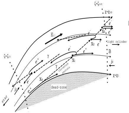
Figure 1: The pair creation cascade model in the meridional plane. The electrons or positrons are accelerated by the electric field along the magnetic field lines and emit the $\gamma$-rays. In the meridional plane, the $\gamma$-rays radiated by the curvature process are beamed in the direction of local magnetic field. The radiated $\gamma$-rays may convert into the pairs by the pair creation process. The new born pairs are also accelerated and emit the $\gamma$-rays. The $\chi_{l}$, $\chi_{up}$, $\zeta_{in}$, and $\zeta_{out}$ present the lower, upper, inner, and outer boundaries of the gap, respectively.

To calculate the source function $S(\mathbf{r})$ and $\gamma$-ray spectrum, we apply the simulation code developed in Paper2 (but we will revise the code for some effects as described later): Step1) We calculate number ($\equiv G_{0}^{i}$) of the emitted photons per unit time per unit volume at position $\mathbf{X}_{0}$ (see Fig.1). The $\gamma$-rays are emitted in the direction of the particle motion $\mathbf{v}$ at $\mathbf{X}_{0}$. Step2) We calculate photon number converted into pairs in a distance $s_{0}(\sim\varpi_{lc})$ by $\delta G^{i}=G_{0}^{i}[1-\exp(-\int_{0}^{s_{0}}1/l_{p}ds^{\prime})]$. Step3) We divide $\delta G^{i}$ photons into $n$ flux elements, and pick up $n$ points on the three-dimensional path length ($s_{i}<s_{0},i=1,\cdots n$) following Monte Carlo method (§§2.4.2). The pair creation point $\mathbf{X}_{i}$ in the meridional plane is deduced from $|\mathbf{X}_{i}-\mathbf{X}_{0}|=s_{i}\cos\theta_{\gamma}$, where $\theta_{\gamma}=\cos^{-1}\sqrt{1-(\Omega\varpi/\varpi_{lc})^{2}}$. Step4) We calculate the number of pairs produced per unit time per unit volume as the source term $S(\mathbf{X}_{i})$.

In this paper, we take into account the following effects:

• the energy spectrum of the curvature photons emitted by the individual particles,

• the soft photon field proportional to the inverse square of the distance (that is, inhomogeneous) and the soft photons propagate radially from the stellar surface (that is, anisotropic),

which were ignored in Paper2 for simplicity. In the following subsections, we detail how the above effects are built onto the cascade model.

2.4.1 Curvature spectrum

To give $G_{0}^{i}$ in Step3), we define the following $\gamma$-ray photon number densities in the dimensionless energy interval between $x_{i}$ and $x_{i+1}$,

$$G_{0}^{i}=\frac{\int_{x_{i}}^{x_{i+1}}P_{c}(x)dx}{(x_{i}+x_{i+1})/2}=\frac{\sqrt{3}e^{2}\Gamma}{hR_{c}}\frac{\int_{x_{i}}^{x_{i+1}}F(x)dx}{(x_{i}+x_{i+1})/2}~{}~{}~{}(i=1,\cdots,n_{1}-1),$$ (25)

where $x_{i}=E_{\gamma}^{i}/E_{c}$. We define $x_{1}=0$ and select each value of $x_{i}$ $(i=2,\dots n_{1})$ so as to satisfy $\int_{x_{i}}^{x_{i+1}}F(x)dx=a_{1}/n_{1}$, where $a_{1}=\int_{0}^{\infty}F(x)dx=8\pi/3^{5/2}$. Instead of $x=\infty$, we define $x_{n_{1}+1}\equiv(3x_{n_{1}}-x_{n_{1}-1})/2$ and $G_{0}^{n_{1}}\equiv a_{1}/x_{n_{1}+1}$. For each bin $G_{0}^{i}$, we carry out the processes Step1)$\sim$Step4). In this paper, we adopt $n_{1}=20$ and $n=20$ in Step3).

2.4.2 Pair creation cascade model

The radial dependence in the mean free path of equation (15) can be written as $l_{p}\propto(1-\cos\theta_{X\gamma})^{-1}r^{2}$, where $r^{2}$ arises due to soft photon field diluting with the radial distance and $\theta_{X\gamma}$ of equation (18) is the collision angle between an $X$-ray photon and a $\gamma$-ray photon. Because $\cos\theta_{X\gamma}\sim\cos\theta_{em}$ is satisfied as long as the propagating distance $s$ is smaller than the radial distance $r\sim 0.5\varpi_{lc}$, the radial dependence of the collision angle for $\gamma$-rays emitted at the same position is less important. In this paper, therefore, we adopt $\theta_{X\gamma}=\theta_{em}$, which are collision angle at the emission point of the $\gamma$-rays considered. We take into account the fact that the value of $\theta_{em}$ depends on the emission point and the emitted direction (inwardly or outwardly) of the $\gamma$-rays.

Using Monte Carlo method, we simulate the pair-creation position in the gap. The probability that a $\gamma$-ray photon makes a pair between distance $s$ and $s+ds$ from the emission point is

$$P_{p}ds=\frac{\exp(-\int_{0}^{s}1/l_{p}(s^{\prime})ds^{\prime})}{l_{p}(s)}ds.$$ (26)

Using a function [$\equiv f(y)$], we transform uniformly distributed random numbers, $\{y_{1},y_{2},\dots,y_{n}\}\equiv\mathbf{y}$, into random numbers, $\{s_{1},s_{2},\cdots,s_{n}\}\equiv\mathbf{s}$, following the probability $P_{p}$. We obtain the function $f(y)$ by solving the equation (Press et al., 1988)

$$\left|\frac{dy}{ds}\right|=\frac{1}{l_{p}}\exp(-\int_{0}^{s}1/l_{p}ds^{\prime}).$$ (27)

For the present case, $l_{p}\propto r^{2}$, we can perform the integration in equation (27) analytically. As a result, we obtain the function $f(y)$ as

$$s=f(y)=r_{0}\sin\theta_{em}\tan\left[-r_{0}\frac{\sin\theta_{em}\mathrm{ln}y}{c_{1}}+\mathrm{atan}\left(\frac{1}{\tan\theta_{em}}\right)\right]-r_{0}\cos\theta_{em},$$ (28)

where

$$c_{1}=(1-\cos\theta_{X\gamma})\frac{2\pi^{2}R^{2}_{eff}}{h^{3}c^{3}}\int_{E_{th}}^{\infty}dE_{\gamma}\frac{E_{X}^{2}}{\exp(E_{X}/kT_{s})-1}\sigma_{p}.$$

The transformation represented by equation (28) gives a random number $s$ of $0<s<\infty$ with a uniformly selected random number $y$ of $0<y<1$. Because we are concerned with the pair creation positions between $0<s<s_{0}\sim\varpi_{lc}$, we define uniformly distributed random numbers as $\mathbf{y}^{1}\equiv(c_{y}-1)\mathbf{y}+1$, where

$$c_{y}=\exp\left\{-\frac{1}{r_{0}\sin\theta_{em}}\left[\mathrm{atan}\left(\frac{s_{0}+r_{0}\cos\theta_{em}}{r_{0}\sin\theta_{em}}\right)-\mathrm{atan}\left(\frac{1}{\tan\theta_{em}}\right)\right]\right\}.$$

A series of the transformations, $\mathbf{y}\Rightarrow\mathbf{y}^{1}\Rightarrow\mathbf{s}=f(\mathbf{y}^{1})$, produces the pair creation positions $\mathbf{s}$ following the probability $P_{p}$ between $0<s<s_{0}\sim\varpi_{lc}$.

Following above Monte Carlo method, we choose $n$ pair-creation positions for $G_{0}^{i}$ photons emitted at the position considered. On each pair-creation position, the pairs produced per unit time and per unit volume is given by $G_{0}^{i}[1-\exp(-\int_{0}^{s_{0}}1/l_{p}ds^{\prime})]/n$.

2.5 Boundary conditions

We introduce the conventional dimensionless variables:

$$\tilde{\mathbf{r}}=\frac{\omega_{p}}{c}\mathbf{r},\ \ \ \ \omega_{p}=\sqrt{\frac{4\pi e^{2}}{m_{e}}\frac{\Omega B_{lc}}{2\pi ce}},$$ (29)

$$\tilde{\Phi}_{nco}=\frac{e}{m_{e}c^{2}}\Phi_{nco},\ \ \ \ \tilde{\mathbf{E}}=-\tilde{\nabla}\tilde{\Phi}_{nco},$$ (30)

$$j_{\pm}=\frac{ev_{||\pm}N_{\pm}}{\Omega B/2\pi},\ \ \ \ \tilde{\mathbf{B}}=\mathbf{B}/B_{lc},$$ (31)

$$\mathbf{\beta}=\frac{\mathbf{v}}{c},$$ (32)

and

$$\tilde{\rho}=\frac{\rho}{\Omega B_{lc}/2\pi c}=\frac{\tilde{B}}{\beta_{||}}(j_{+}-j_{-}),\ \ \ \ \tilde{\rho}_{GJ}=-\tilde{B}_{z}.$$ (33)

The Poisson equation (4) and the continuity equation (14) are rewritten as

$$\tilde{\triangle}\tilde{\Phi}_{nco}=-[\frac{\tilde{B}}{\beta_{||}}(j_{+}-j_{-})+\tilde{B}_{z}],$$ (34)

and

$$\tilde{\mathbf{B}}\cdot\tilde{\nabla}j_{\pm}=\pm\tilde{S}(\tilde{\mathbf{r}}),$$ (35)

respectively.

In the meridional plane, the outer gap has four boundaries called as upper, lower, inner and outer boundaries (see Fig.1). The upper and lower boundaries are defined by the magnetic surfaces labeled by $\chi_{up}$ and $\chi_{l}$, respectively. The inner $[\equiv\zeta_{in}(\chi)]$ and outer $[\equiv\zeta_{out}(\chi)]$ boundaries are functions of $\chi$. For example, $\zeta_{out}(\chi)$=constant represents the outer boundary defined by a curve line perpendicular to the magnetic field lines.

We impose some conditions on the four boundaries. The inner and the outer boundaries are defined by the surfaces on which the field-aligned electric field $\tilde{E}_{||}$ vanishes,

$$\tilde{E_{||}}(\zeta_{in})=\tilde{E_{||}}(\zeta_{out})=0.$$ (36)

With $Con$3 in §2, we have postulated that the condition $\tilde{\mathbf{E}}\cdot\tilde{\mathbf{B}}=0$ holds between the stellar surface and the outer gap. The uniform value of $\tilde{\Phi}_{nco}$ over the stellar surface propagates to the inner, upper and lower boundaries. By setting an arbitrary constant for $\tilde{\Phi}_{nco}$ on the stellar surface to be zero, we impose

$$\tilde{\Phi}_{nco}(\zeta_{in})=\tilde{\Phi}_{nco}(\chi_{up})=\tilde{\Phi}_{nco}(\chi_{l})=0.$$ (37)

As discussed in §§4.3, there is a possibility that the condition $\tilde{\mathbf{E}}\cdot\tilde{\mathbf{B}}=0$ is not held between the stellar surface and the inner boundary. For such a case, it is difficult to determine the boundary condition on the inner boundary of the outer gap. However, because the potential drop between the stellar surface and the inner boundary is expected much smaller than the potential drop of whole outer gap as discussed in §§4.3, the condition (37), $\tilde{\Phi}_{nco}=0$, at the inner boundary is a good treatment.

The continuity equation (35) satisfies the conservation law of the longitudinal current density, that is, the total current density $j_{+}+j_{-}$($\equiv j_{tot}$) is constant along a field line. This total current $j_{tot}$ can be rewritten by sum of external and internal components. The external component is separated into two parts:

1. $j_{1}$, the current carried by the positrons (e.g. originating in sparking on the stellar surface) coming into the gap through the inner boundary,

2. $j_{2}$, the current carried by the electrons (e.g. originating in pulsar wind region) coming into the gap through the outer boundary.

In the following, we call $j_{1}$ and $j_{2}$ as the external positron and electron components, respectively. The internal component ($\equiv j_{g}$) is carried by the electrons and positrons produced in the gap. In terms of $(j_{g},j_{1},j_{2})$, the total current density becomes

$$j_{tot}(\chi)=j_{1}(\chi)+j_{2}(\chi)+j_{g}(\chi).$$ (38)

The current should be determined by some global conditions, because the outer gap, the polar cap and the pulsar wind interact each other through the current. By parameterizing external positron and electron components, we impose the conditions as follows

$$j_{+}(\zeta_{in})=j_{1}(\chi),$$ (39)

and

$$j_{-}(\zeta_{out})=j_{2}(\chi).$$ (40)

We have four model parameters, i.e. the inclination angle ($\alpha_{inc}$) and the three current components $(j_{1},j_{2},j_{g})$. Because we have Dirichlet-type and Neumann-type conditions on the inner boundary, we solve the position of the inner boundary. We fix the lower boundary to the last open line. In the present model, we obtain unique positions of the inner and outer boundaries by giving the three current components and the position of the upper boundary. In the calculation, however, we give the position of the outer boundary instead of the internal current ($j_{g}$) and solve the trans-field distribution of $j_{g}$, because it is difficult to manage the distribution of $j_{g}$, which is affected by the pair creation cascade, by hand.

We consider the following particular solution in the present paper. In general, the internal current $j_{g}$ increases as the outer boundary shifts toward the light cylinder if one fixes the position of the upper boundary. In the present electrodynamical model, the solutions satisfying the boundary conditions disappear if a large internal current $j_{g}$ flows on a magnetic field line. We regard that the gap having a marginal structure represents the state that actually appearers. This critical value of the internal current component is denoted by $j_{crit}$. If one gives the position of the upper boundary ($\chi_{up}$) and the external current components ($j_{1},j_{2}$), the trans-field distribution of $j_{g}$ having the critical internal components $j_{crit}$ and the positions of the inner ($\zeta_{in}$) and outer ($\zeta_{out}$) boundaries are determined.

As we just mentioned, the solutions satisfying the boundary conditions disappear if the internal component $j_{g}$ becomes too large ($>0.1\sim 0.2$), because the produced pairs may make the super Goldreich-Julian charge density and may quench the gap. On the other hand, we can significantly increase the external component $j_{1}$ or $j_{2}$ because the injected particles only shift the gap outward and inward. For example, if the external electron component $j_{2}$ increases, the effective charge neutral surface and the outer gap position shift inside relative to the conventional null charge surface of the Goldreich-Julian charge density (see §§3.1).

A solution is given by a self-consist connection between the field-aligned electric field determined by the distribution of the charge density (i.e. the pair creation cascade), the pair creation cascade controlled by the curvature radiation process (i.e. the Lorentz factor in the gap), and the Lorentz factor calculated from the electric field.

The expected $\gamma$-ray flux on the Earth is given by

$$F(E_{\gamma})=\frac{1}{\triangle\Omega d^{2}}N_{\gamma}(E_{\gamma})$$ (41)

where $\triangle\Omega$ is solid angle of the $\gamma$-ray beam and $N_{\gamma}(E_{\gamma})$ is the total photon number emitted per unit energy per unit time,

$$N_{\gamma}(E_{\gamma})=\int_{V_{tot}}\frac{P_{c}(\mathbf{r},E_{\gamma})N_{\pm}(\mathbf{r})}{E_{\gamma}}dV,$$ (42)

where $V_{tot}$ represents the total volume of the emission region, which includes both inside and outside the gap. In the present two-dimensional model, the solid angle of the $\gamma$-ray beam is estimated as $\triangle\Omega\sim 2\pi D_{\perp}/r_{out}$, where $D_{\perp}$ and $r_{out}$ are, respectively, the solved trans-field thickness and the radial distance to the outer boundary of the outer gap. The total photon number $N_{\gamma}(E_{\gamma})$ emitted in the gap depends on the azimuthal spread angle ($\equiv\triangle\phi$) of the outer gap, which is unsolved in the present model. Because there are no detail discussions for the pair creation cascade process with the three dimensional geometry up to now, it is difficult to estimate the azimuthal spread angle of the gap in the present two-dimensional model. Therefore, we use the azimuthal spread angle as a model parameter to be determined by the observed flux. The observed emission phase in the light curves (Kanback et al. 1994; Fierro et al. 1998) and the previous geometrical studies (Romani 1996; Cheng et al. 2000) for the light curves model have predicted $\triangle\phi\sim\pi$ radian.

3 Results

In this section, we present the results where we use the parameters of the Vela pulsar whose $X$-ray field at the outer gap is deduced from the observations. From $ROSAT$ (Ögelman, Finley & Zimmerman 1993), $RXTE$ (Harding et al. 2002) and $Chandra$ (Pavlov et al. 2001) observations of the Vela pulsar, the spectrum in $X$-ray band is expressed by two components; power-low component and surface black body component. Because the former component is much fainter than the latter component, we neglect the former contribution to the $X$-ray field of the pair creation process. Ögelman et al.(1993) fitted the thermal component with $T^{\infty}\sim 1.7$ MK and $R_{eff}\sim 1.3(d/0.25\mathrm{kpc})^{2}$ km, where $d$ is the distance to the Vela pulsar. In this paper, we adopt $T^{\infty}=1.7$ MK and $d=0.25$ kpc (Cha, Semback & Danksm 1999).

In the following subsections, we examine the dependence of the $\gamma$-ray spectrum on the current components by fixing firstly the critical internal component $j_{crit}$ (§§3.1) and secondly the external components, $j_{1}$ and $j_{2}$ (§§3.2). In §§3.3, we compare the results with the observed spectrum of the Vela pulsar, and diagnose the outer gap geometry, the current and the inclination angle.

3.1 Gap structures for various external components

Figure 2: The trans-field structures of the internal component $j_{g}$ for $\mathrm{case}_{45}$1$\sim$$\mathrm{case}_{45}$ 4.

In this subsection we fix the inclination angle at $\alpha_{inc}=45^{\circ}$ and the critical internal component at $j_{crit}\sim 0.12$. To examine the effects of the external components ($j_{1},j_{2}$), we consider the following four cases:

1. $(j_{1},j_{2})=(10^{-5},10^{-5})$ for $\chi_{up}\geq\chi\geq\chi_{l}$,

2. $(j_{1},j_{2})=(0.05,0.05)$ for $\chi_{up}\geq\chi\geq\chi_{l}$,

3. $(j_{1},j_{2})=(0.1,0.0)$ for $\chi_{up}\geq\chi\geq\chi_{l}$,

4. $(j_{1},j_{2})=(0.0,0.1)$ for $\chi_{up}\geq\chi\geq\chi_{l}$.

In $\mathrm{case}_{45}$ 2$\sim$$\mathrm{case}_{45}$ 4, the external current is 10% of the Goldreich-Julian value, which is carried by both components (for $\mathrm{case}_{45}$ 2), the positron component (for $\mathrm{case}_{45}$ 3), and the electron component (for $\mathrm{case}_{45}$ 4). In $\mathrm{case}_{45}$ 1, we consider a case of very small external component, that is, whole current is carried by the internal component, $j_{tot}(\chi)\sim j_{g}(\chi)$.

Fig.2 shows the trans-field distribution of the internal component $j_{g}$ for $\mathrm{case}_{45}$ 1$\sim$$\mathrm{case}_{45}$ 4. The abscissa and ordinate refer, respectively, the current density in units of the Goldreich-Julian value and the hight from the last open line (i.e. the lower boundary). The total current density on each magnetic field line is represented by $j_{tot}(\chi)=j_{g}(\chi)+j_{1}+j_{2}$. So, for each case, the total current density on the magnetic field line where the internal component has the critical value ($j_{crit}\sim 0.12$) is $j_{tot}\sim 0.12$ for $\mathrm{case}_{45}$ 1 ($j_{1}=j_{2}=0$) and $j_{tot}\sim 0.22$ for $\mathrm{case}_{45}$ 2$\sim$$\mathrm{case}_{45}$ 4 ($j_{1}+j_{2}=0.1$).

3.1.1 General features

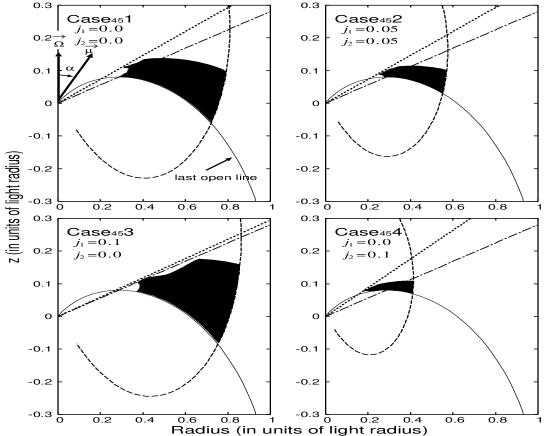
Figure 3: The geometries of the outer gap (filled region in each panel) for $\mathrm{case}_{45}$ 1$\sim$$\mathrm{case}_{45}$ 4. The solid and dashed and dashed-dotted lines show the last open line, the curve line representing the outer boundary and the conventional null charge surface, respectively. On the dotted line in each panel, the condition, $j_{crit}+j_{2}-j_{1}=\tilde{B}_{z}/\tilde{B}$, where $j_{crit}\sim 0.12$, is satisfied .

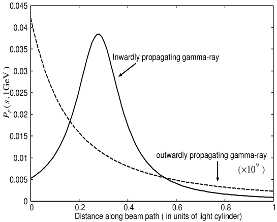
Figure 4: Par-creation probability of a $\gamma$-ray with 1GeV emitted from the null point on the last open line. The solid and dashed lines refer, respectively, the probability of the inwardly and outwardly propagating $\gamma$-rays in the Vela magnetosphere. The dashed line shows the value increased $10^{9}$ times of the probability.

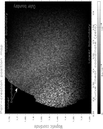
Figure 5: The pair creation position map in the gap of $\mathrm{case}_{45}$ 2. The whiteness refers the particles flux (divided by $\Omega B/2\pi e$) produced per unit length [/cm] due to the pair creation at each position.

The filled regions in Fig.3 show the outer gap in the magnetosphere for $\mathrm{case}_{45}$ 1$\sim$$\mathrm{case}_{45}$ 4. The inner boundary in each panel satisfies both conditions $\tilde{E}_{||}=0$ and $\tilde{\Phi}_{nco}=0$. The solid and dashed-dotted lines in each panel are the last open line and the conventional null charge surface, respectively. The outer boundaries of $\mathrm{case}_{45}$ 1, 2, 3, and 4 are defined by the curved lines (the dashed lines) labeled by $\zeta_{out}\sim 0.9$, $\sim$0.65, $\sim$0.95, and $\sim 0.45$, respectively.

We list the general features that were already detailed in Paper2, in which $\alpha_{inc}$=0^∘:

• The external component affects the gap position in the pulsar magnetosphere. As appeared in Fig.3, the typical gap position of $\mathrm{case}_{45}$ 3 or $\mathrm{case}_{45}$ 4 is shifted outside or inside relative to the typical positions of $\mathrm{case}_{45}$ 1 and $\mathrm{case}_{45}$ 2. Specifically, if $j_{1}=j_{2}$ such as $\mathrm{case}_{45}$ 1 and $\mathrm{case}_{45}$ 2, the inner boundary of the lower parts of the gap, where $j_{g}\sim 0$, is located close to the conventional null charge surface ($\rho_{GJ}=0$). On the other hand, if $j_{1}\neq j_{2}$ such as $\mathrm{case}_{45}$ 3 or $\mathrm{case}_{45}$ 4, the outer boundary shits outside or inside. This is because the external component shifts the effective charge neutral surface relative to the conventional null surface.

• As the dotted lines, on which $j_{crit}+j_{2}-j_{1}=\tilde{B}_{z}/\tilde{B}$ with $j_{crit}\sim 0.12$ is satisfied, shows, the cusp of the inner boundary of each case is located at the position where the space charge density caused by the current is equal to the local Goldreich-Julian charge density. The inner boundary shifts toward the stellar surface as the critical and/or external electron components increases.

• As Fig.2 shows, the present model predicts that more large current runs though the middle part of the gap rather than the upper part predicted in the CHR86 arguments. The internal component $j_{g}$ increases with hight in the lower half part of the gap, and decreases in the upper half part. This decrease is because most $\gamma$-rays emitted in the lower part of the gap escape from the inner boundary or the outer boundary before reaching the upper part. Another reason is that the field-aligned electric field, the Lorentz factor and in turn the emitted photon energy decrease with increasing hight in the upper half part.

3.1.2 Gap geometry & pair creation mean-free path

In Paper2, the trans-field thickness of the outer gap was not sensitive to the external component (for example fig.6 in Paper2), because we assumed a homogeneous $X$-ray field. On the other hand, we find in Fig.3 that the trans-field thicknesses of $\mathrm{case}_{45}$ 2 and $\mathrm{case}_{45}$ 4 are much smaller than those of $\mathrm{case}_{45}$ 1 and $\mathrm{case}_{45}$ 3. This difference in the thickness is explained in terms of the mean-free path depending on the radial distance and the emission direction, which were ignored in Paper2, as follows.

Fig.4 shows how the pair-creation probability of equation (26) develops along the path of 1GeV $\gamma$-rays emitted from the null point on the last open line. The solid and dashed lines refer the probabilities of a photon emitted inward and outward, respectively. The dashed line shows the value increased $10^{9}$ times of the probability. We find that the mean free path of the outwardly propagating $\gamma$-rays is much longer than that of the inwardly propagating ones, in which a photon out of about $10^{3}$ photons converts into a pair after running about the light radius. Fig.5 shows the pair creation position map of $\mathrm{case}_{45}$ 2 ($j_{1}=j_{2}=0.05$), where we do not plot the pairs created outside the gap. In Fig.5, the increase in the whiteness refers the pair flux produced per unit length at each position. As we expected, the inwardly propagating $\gamma$-rays make many pairs around the inner boundary and the middle part of the gap.

The large difference in the mean-free path between the outwardly and inwardly propagating $\gamma$-rays is mainly attributed to difference in the collision angle $\theta_{X\gamma}$ with the surface X-ray photon. For example, the collision angle of the $\gamma$-ray photon emitted from the conventional null point on the last open line of $\alpha_{inc}=45$^∘ becomes $\theta_{X\gamma}\sim 22.8$^∘ for the outwardly propagating and becomes $\theta_{X\gamma}\sim 157.2$^∘ for the inwardly propagating $\gamma$-rays. So, the pair creation processes occur with tail-on like collision ($1-\cos\theta_{X\gamma}\sim 0$) for the outwardly and head-on like collision ($1-\cos\theta_{X\gamma}\sim 2$) for the inwardly propagating $\gamma$-rays. For the outwardly propagating $\gamma$-rays with 1GeV, the threshold energy of the $X$-ray photon of the pair creation is given by $E_{th}=2(m_{e}c^{2})^{2}/(1-\cos\theta_{X\gamma})/\mathrm{1GeV}\sim 6.7$keV, which indicates the deep Wien region of the Planck distribution for the Vela pulsar ($kT_{s}\sim 0.15$keV). For the inwardly propagating $\gamma$-rays, the threshold energy becomes $E_{th}\sim 0.27$keV. This difference in the threshold energy and the resultant difference in the $X$-ray photon number for the collision mainly produce the large difference in the mean free path.

Because a large production of the pairs immediately quenches the gap, the mean-free path of the pair creation controls the gap size. As a results, $\mathrm{case}_{45}$ 2 and $\mathrm{case}_{45}$ 4, in which many $\gamma$-rays are emitted inward by the external electrons, have much smaller gap thickness than $\mathrm{case}_{45}$ 3, in which many $\gamma$-rays are emitted outward by the external positrons.

3.1.3 Electric structure

Figure 6: The electric field structure for $\mathrm{case}_{45}$ 1$\sim$$\mathrm{case}_{45}$ 4. The solid, dotted, and dashed lines in each panel show the distribution of the field-aligned electric field on the three different magnetic field lines, which locate, respectively, 25, 50, and 75% of the gap trans-field thickness measured from the last open field line. The abscissa represent the arc length with the origin at the null surface.

Fig.6 shows the distribution of the field-aligned electric field along the magnetic field lines for $\mathrm{case}_{45}$ 1$\sim$$\mathrm{case}_{45}$ 4. The solid, dotted and dashed lines represent, respectively, the field-aligned electric field on the magnetic field through the gap at 25, 50 and 75% of the trans-field thickness from the lower boundary. The abscissa refers the arc length from the conventional null charge surface, where the positive and negative values indicate outside and inside, respectively, with respect to the null surface.

Combining Fig.3 and Fig.6, we find a tendency that the field-aligned electric field becomes strong with increasing trans-field thickness. For example, in $\mathrm{case}_{45}$ 2, $\mathrm{case}_{45}$ 3 and $\mathrm{case}_{45}$ 4, in which $j_{tot}\sim 0.2$, $\mathrm{case}_{45}$ 3 has both the largest trans-field thickness and the strongest field-aligned electric field, on the other hand, $\mathrm{case}_{45}$ 4 has both smallest trans-field thickness and the weakest field-aligned electric field. The available potential drop ($\equiv\delta\Phi_{a}$ ) in the outer gap may be written as $\delta\Phi_{a}\sim\Phi_{a}\delta\theta_{gap}/\theta_{p}$, where $\Phi_{a}$ is the available potential drop on the stellar surface, $\delta\theta_{gap}$ is the angle of the foot points of the open field lines through the gap, and $\theta_{p}$ is the angle of the polar cap. Because the angle $\delta\theta_{gap}$ increases with the trans-field thickness, the potential drop increases with the trans-field thickness. As shown in Paper2, the strength of the field-aligned electric field does not depend on the gap width along the field lines very much, because the effective charge density $(j_{+}-j_{-})\tilde{B}/\beta_{||}+\tilde{B}_{z}$ and the transverse term $-\tilde{\triangle}_{\perp}\tilde{\Phi}_{nco}$ in the Poisson equation almost balance out in the gap (§§2.1). As a results, the strength of the electric field tends to increase with the trans-field thickness. This effect is originally pointed out by the vacuum gap model of CHR86.

From Fig.3 and Fig.6, we also find that the field-aligned electric field of $\mathrm{case}_{45}$ 3 is weaker than that of $\mathrm{case}_{45}$ 1, although the trans-field thickness of $\mathrm{case}_{45}$ 3 is larger. This reflects the screening effects of the particles on the field-aligned electric field. The dimensionless effective charge densities near the outer boundary for $\mathrm{case}_{45}$ 1 and $\mathrm{case}_{45}$ 3 are written as $\tilde{\rho}_{eff}=\tilde{B}j_{g}/\beta_{||}-\tilde{B}_{z}$ and $\tilde{\rho}_{eff}=\tilde{B}(j_{g}+j_{1})/\beta_{||}-\tilde{B}_{z}$, respectively. For $\mathrm{case}_{45}$ 3, the external positrons assist in the screening near the outer boundary.

As we have seen, the combination of the effects of the gap thickness and the screening of the particles determine the strength of the field-aligned electric field in the gap.

3.1.4 $\gamma$-ray spectrum

Figure 7: Calculated $\gamma$-ray spectra of the curvature radiation for $\mathrm{case}_{45}$ 1$\sim$$\mathrm{case}_{45}$ 4 of the Vela pulsars. The solid line show the expected spectrum, which are composed of the inside (dashed line) and outside (dotted line) emissions. The crosses show the $EGRET$ phase-averaged spectrum. The parameter $\triangle\phi$ adjusts the calculated flux to the observation.

As we see in Fig.5, because most pairs are created near the inner boundary, the emission region for the inwardly $\gamma$-rays in the gap is restricted around the inner boundary, while the emission region for the outwardly $\gamma$-rays is whole outer gap. Furthermore, we expect that almost inwardly propagating $\gamma$-rays are converted into pairs by the magnetic or photon-photon pair creations when they pass close to the star. Therefore, we assume that the contribution of the inwardly $\gamma$-rays to the spectrum on the Earth is ignorable.

Fig.7 shows the calculated curvature spectra of the outwardly propagating $\gamma$-rays for $\mathrm{case}_{45}$ 1$\sim$$\mathrm{case}_{45}$ 4. The solid lines in Fig.7 represent the expected spectrum, which are composed of the gap emissions (dashed line) and the emissions (dotted line) from outside the gap. The crosses in Fig.7 show the $EGRET$ phase-averaged spectrum of the Vela pulsar. The adjusted azimuthal spread angle to the observed flux for each case is $\triangle\phi\sim 25$ radian ($\mathrm{case}_{45}$ 1), $\sim 12$ radian ($\mathrm{case}_{45}$ 2), $\sim 6$ radian ($\mathrm{case}_{45}$ 3) and $\sim 43$ radian ($\mathrm{case}_{45}$ 4).

From Fig.7, we find that the outside emissions (dotted lines) of $\mathrm{case}_{45}$ 1 and $\mathrm{case}_{45}$ 3 are fainter than the inside emissions (dashed lines). As the outer gap geometries in Fig.3 show, the outer boundary of $\mathrm{case}_{45}$ 1 or $\mathrm{case}_{45}$ 3 is located near the light cylinder. Therefore, the outside emission region is smaller than the outer gap. For $\mathrm{case}_{45}$ 2 and $\mathrm{case}_{45}$ 4, on the other hand, the outside emissions contribute to the total spectrum below 1GeV, because the size of the outside emission region is similar to or larger than the gap size.

Combining Fig.6 and Fig.7, we see that the spectral hardness reflects directly the strength of the field-aligned electric field. For example, the strongest (or weakest) electric field of $\mathrm{case}_{45}$ 1 (or $\mathrm{case}_{45}$ 4) in all cases produces the hardest (or softest) spectrum. We find that the spectrum becomes to be soft as the currents increase. Especially, by comparing the spectra of $\mathrm{case}_{45}$ 1 and $\mathrm{case}_{45}$ 4, we see that the spectrum sharply softens as the electron injection at the outer boundary increases. By comparing the spectra of $\mathrm{case}_{45}$ 1 and $\mathrm{case}_{45}$ 3, on the other hand, we also find that the increasing in the positronic component gradually softens the spectrum.

3.2 Dependence on the internal current $j_{g}$

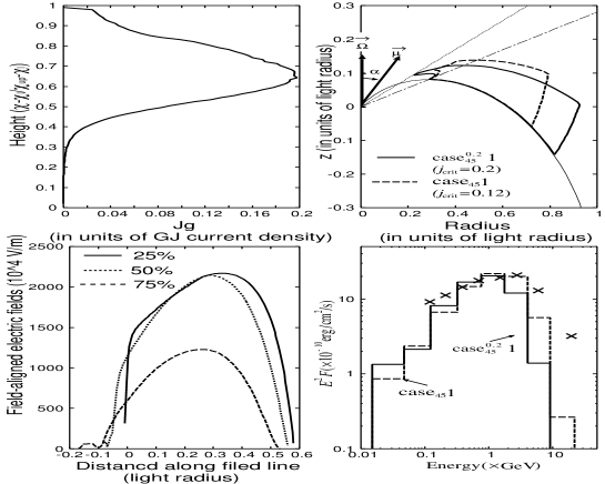
Figure 8: The solved outer gap ($\mathrm{case}_{45}^{0.2}~{}1$) of $(j_{1},j_{2})=(0,0)$ and $j_{crit}\sim 0.2$. The solid line in each panel shows the trans-field distribution of the internal current (upper left), the gap geometry (upper right), distribution of the field-aligned electric field (lower left) and the total spectrum (lower right). For comparison, we also display the gap geometry and the total spectrum of $\mathrm{case}_{45}$ 1.

In the last section, we have investigated the dependence of the spectral hardness on the external components $(j_{1},j_{2})$. To clear the dependence of the spectrum on the critical internal component $j_{crit}$, we also calculate the case that $j_{1}=j_{2}=10^{-5}$ and $j_{crit}\sim 0.2$ (denoted as $\mathrm{case}_{45}^{0.2}~{}1$) and compare the results with that of $\mathrm{case}_{45}$ 1 ($j_{1}=j_{2}=10^{=5},j_{crit}\sim 0.12$). The results of $\mathrm{case}_{45}^{0.2}~{}1$ are summarized in Fig.8. The upper left, upper right, lower left and lower right panels show the trans-field distribution of the internal component, the gap geometry, the distribution of the field-aligned electric field, and the total spectrum, respectively. For comparison, we also display the gap geometry and the total spectrum of $\mathrm{case}_{45}$ 1 with dashed lines in Fig.8.

As Fig.8 shows, the larger critical internal component, that is $\mathrm{case}_{45}^{0.2}~{}1$, is predicted by a gap having the smaller trans-field thickness and longer width along the magnetic field lines. We expect that the gap of $\mathrm{case}_{45}^{0.2}~{}1$ has a longer gap width $W_{||}$ than that of $\mathrm{case}_{45}$ 1, because the internal component $j_{g}$ increases with the gap width. For $\mathrm{case}_{45}$ 1, we adjust the positions of the outer and upper boundaries so as to reproduce a marginal gap structure having $j_{crit}\sim 0.12$. The field-aligned electric field changes it’s sign in the gap due to the screening effect of the particles if we shift the outer boundary outward relative to that of $\mathrm{case}_{45}$ 1 without changing the upper boundary. As Fig.8 shows, therefore, the gap of $\mathrm{case}_{45}^{0.2}~{}1$ has a smaller thickness and a longer width than those of $\mathrm{case}_{45}$ 1.

The decrease of the gap thickness causes a large transverse term $\triangle_{\perp}\Phi_{nco}\sim-\Phi_{nco}/D_{\perp}^{2}$. As discussed in Paper2, the transverse term reduces the screening effects of the electrons, because it acts as a positive charge in the Poisson equation. The internal component $j_{g}$ can increase until the transverse term marginally sustain the negative charged super-GJ region, where $|\rho|>|\rho_{GJ}|$, in the gap. The choice of a large critical internal component tends to result in a smaller thickness.

Because the smaller trans-field thickness gives the smaller field-aligned electric field and furthermore because the larger internal component $j_{g}$ gives the stronger screening effects for the field-aligned electric field, the resultant $\gamma$-ray spectrum of $\mathrm{case}_{45}^{0.2}~{}1$ is softer than that of $\mathrm{case}_{45}$ 1.

We summarize the discussions in §§3.1 and §§3.2. The spectrum becomes soft as the current components, ($j_{crit},j_{1},j_{2}$), increase due to the screening effect on the field-aligned electric field. Especially, the increase in the electron component $j_{2}$ at the outer boundary sharply softens the spectrum. On the other hand, the increase in the positronic component $j_{1}$ at the inner boundary gradually softens the spectrum. By increasing the positronic component $j_{1}$, therefore, we can obtain a brighter emission with similar spectral hardness (see §§§3.3.2). This dependence of the spectral feature on the current allow us to diagnose what current flows in the gap of the observed $\gamma$-ray pulsars.

3.3 Application to the Vela pulsar

In the present two-dimensional model, the gap width and thickness are linked so that we can discuss the gap structure in terms of the spectral characteristic; i.e. the cut-off energy and the flux. By comparing the model spectra with the observed spectrum, we can diagnose the free model parameters, that is, the current components $(j_{crit},j_{1},j_{2})$ and the inclination angle $\alpha_{inc}$. In this paper, we apply the theory to the Vela pulsar.

In §§§3.3.1, we study that the $EGRET$ spectrum of the Vela pulsar predicts the cases that have only a few electron injections ($j_{2}\sim 0$) at the outer boundary. In §§§3.3.2, we discuss parameter spaces of $\alpha_{inc}$ and $j_{1}$, which explain the $EGRET$ spectrum, with $j_{crit}\sim 0.1$, which is moderate value in the present electrodynamical model.

3.3.1 Flow pattern of the external current

From Fig.7, we find that the spectrum of $\mathrm{case}_{45}$ 2, in which $j_{1}=j_{2}=0.05$, $j_{crit}\sim 0.12$ and $\alpha_{inc}=45^{\circ}$, becomes to be very soft as compared with the observation; the spectral cut-off energy is $\sim 0.5$GeV for $\mathrm{case}_{45}$ 2 and $\sim 3$GeV for the observation. We also find that the adjusted spread angle for $\mathrm{case}_{45}$ 2, $\triangle\phi\sim 12$ radian, is unrealistic. Starting from these facts, we can rule out any outer gap having a large particle injection at the outer boundary for the Vela pulsar, as follows.

Firstly, we do not expect the cases having a larger current components than that of $\mathrm{case}_{45}$ 2, because the spectrum softens as the current increases as discussed in §§3.1 and §§3.2.

Secondly, we do not expect the cases that the electronic component $j_{2}$ is the same with that of $\mathrm{case}_{45}$ 2, but the positronic component $j_{1}$ and/or the internal component $j_{crit}$ are smaller than those of $\mathrm{case}_{45}$ 2. This is because the adjusted azimuthal angle $\triangle\phi$ increases with the decreasing $j_{1}$ and/or $j_{crit}$ due to decrease of the outwardly migrating particles. Therefore, the unreality on the spread angle such as $\triangle\phi=12$ radian of $\mathrm{case}_{45}$ 2 grows with decreasing $j_{1}$ and/or $j_{crit}$.

Finally, we can show that the hardness of the spectrum does not depend on the inclination angle very much. The increase in the inclination angle shifts the null point on the last open line toward the stellar surface. This shift increases the strength of the magnetic field in the outer gap, and also decreases the gap thickness with the mean-free path because the $X$-ray field becomes dense and because the collision of the inwardly propagating $\gamma$-rays approaches the head-on. The former effect tends to increase the strength of the field-aligned electric field, the latter to decrease it, the two effects compensate each other. As a results, the spectral hardness does not depend on the inclination angle very much. In fact, there is a tendency that the spectral hardness softens with the inclination angle for the large electron component at the outer boundary. Therefore, we can rule out any inclination angles with $j_{2}\geq 0.05$ for the Vela pulsar.

As a result of the above three arguments, we can rule out any large electronic injection cases, $j_{2}\geq 0.05$, and we suggest that only a few electrons ($j_{2}\sim 0.0$) are injected into the gap at the outer boundary for the Vela pulsar.

For $j_{2}\sim 0$, the decreasing of the gap thickness with increasing the inclination angle is more moderate than the case of the large external electron case, because the mean free path of the outwardly $\gamma$-rays is very longer than the gap thickness. As a results, we can see that the strength of the field-aligned electric field and resultant hardness of the spectrum tend to increase with the inclination angle for $j_{2}\sim 0$.

3.3.2 Diagnosis the current and the inclination angle

Figure 9: The calculated outer gap geometry in wide parameter space 45^∘$<\alpha_{inc}<$75^∘. We use $j_{2}=0$ and $j_{cirt}\sim 0.1$. The thin solid and dotted-dashed lines show the last-open line and the conventional null charge surface, respectively.

Figure 10: The calculated total spectra with various inclination angles and positron components. The external electron and critical internal components are $j_{e}=0$ and $j_{crit}\sim 0.1$. The calculated spectral hardness is explained with $j_{1}\leq 0.08$ for $\alpha_{inc}=45^{\circ}$, $\leq 0.10$ for $\alpha_{inc}=55^{\circ}$, $\leq 0.15$ for $\alpha_{inc}=65^{\circ}$ and $\leq 0.20$ for $\alpha_{inc}=75^{\circ}$.

Following the discussion in §§§3.3.1, we fix the external electron component $j_{2}$ at zero for the Vela pulsar. For $j_{2}\sim 0$ with the present model, the solutions disappear if the critical internal component $j_{crit}$ exceed several ten percent of the Goldreich-Julian value. In this subsection, therefore, we adopt $j_{crit}=0.1$ as a moderate value. With $j_{crit}=0.1$ and $j_{2}=0$, we diagnose other two model parameters, that is, the external positron $j_{1}$ and the inclination angle $\alpha_{inc}$.

Fig.9 and Fig.10 shows the gap geometries and the spectra, respectively, for various positronic components and the inclination angles; upper left panel summarizes the results of $j_{1}=0.01$ (solid), 0.05 (dashed) and 0.08 (dashed) with $\alpha_{inc}=45$^∘, upper right panel $j_{1}=0.01$ (solid), 0.05 (dotted) and 0.1 (dashed) with $\alpha_{inc}=55$^∘, lower left panel $j_{1}=0.05$ (solid), 0.10 (dotted) and 0.15 (dashed) with $\alpha=65$^∘ and lower right panel $j_{1}=0.10$ (solid), 0.15 (dotted) and 0.20 (dashed) with $\alpha_{inc}=75$^∘. By comparing the observed cut-off energy, we can restrict the positronic component $j_{1}$ such as $j_{1}\leq 0.08$ for $\alpha_{inc}=45$^∘, $\leq 0.1$ for 55^∘, $\leq 0.15$ for 65^∘, and $\leq 0.20$ for 75^∘. The result of the marginal case for each inclination angle is shown with the dashed line. The values of the azimuthal spread angle $\triangle\phi$ of the gap written in Fig.9 and Fig.10 are adjusted to the observed flux.

We notice that the increase in the inclination angle permits larger positronic component $j_{1}$. For only a few electronic injections at the outer boundary $j_{2}\sim 0$, the field-aligned electric field in the gap tends to become strong with increasing the inclination angle as described in §§§3.3.1. Stronger field-aligned electric field makes us possible to have larger positronic component $j_{1}$, because we can increase $j_{1}$ until the particles screen the field-aligned electric field so that the calculated spectral cut-off energy does not explain the observation.

For each positron external component $j_{1}$ of $\alpha_{inc}=45^{\circ}$ and $\alpha_{inc}=55^{\circ}$ in Fig.9, the adjusted azimuthal angles $\triangle\phi$ are near or lager than $2\pi$ radian which are unrealistic. Therefore, we do not expect any cases of the critical internal component of $j_{crit}\sim 0.1$, which has been assumed in Fig.9, for $\alpha_{inc}=45^{\circ}$ and $\alpha_{inc}=55^{\circ}$. For smaller critical internal component than $j_{1}\sim 0.1$, the unreality of the azimuthal angle increases. For more large critical internal component such as $j_{crit}\sim 0.2$ of $\mathrm{case}_{45}^{0.2}~{}1$ in §§3.2, the calculated spectra become to be soft as compared with the observation. On these ground, therefore, we safely rule out any cases of $\alpha_{inc}\leq 55^{\circ}$ for the Vela pulsar.

For $\alpha_{inc}=65$^∘, The adjusted azimuthal angle $\triangle\phi\sim 4$ radian of the marginal case (dashed line) is slightly larger than $\triangle\phi\sim\pi$. Because the three-dimensional gap geometry affects the solid angle of the $\gamma$-ray beam and the expected flux on the Earth, we could deem the cases of $\alpha_{inc}=65$^∘ acceptable for the Vela pulsar in the present two-dimensional model. We expect that the large positron component such as $j_{1}\sim 0.1$ runs through in the gap.

For $\alpha_{inc}=75^{\circ}$, the adjusted azimuthal angle of $\triangle\phi\sim 2.5$ radian for $j_{1}=0.2$ explains the observation very well. Furthermore, for $j_{1}=0.1$ (the solid line), the expected angle $\triangle\phi\sim 2.8$ radian is also consistent with the observation. Therefore, we find that both the observed spectral cut-off energy and flux are explained by $j_{1}\leq 0.2$ for $\alpha_{inc}=75$^∘. As we have seen, the upper limit $j_{1}=0.2$ for $\alpha_{inc}=75$^∘ is determined by the spectral cut-off energy. On the other hand, the lower limit of the external positron $j_{1}$ is determined by a comparison between the model and the observed flux. Because the expected flux depends on the three-dimensional geometry, we should use a three-dimensional model to give the lower limit of $j_{1}$ for $\alpha_{inc}=75^{\circ}$.

In summary, we have shown by solving the two-dimensional gap structure that the strength of the field-aligned electric field and the hardness of the produced $\gamma$-ray spectrum are strongly affected by the current through the gap. By comparing the model spectrum with the $EGRET$ observation, we have successfully constrained the model parameters (the current and the inclination angle) for the Vela pulsar, as follows. Only a few external electrons (i.e. $j_{2}\sim 0$) injected into the gap at the outer boundary are predicted by the $EGRET$ observation. We also safely rule out any cases of $\alpha_{inc}\leq 55$^∘. With uncertainty due to the three dimensional effects, we conclude that the Vela pulsar has the inclination angle $\alpha_{inc}$ greater than $65^{\circ}$. With the moderate critical internal component $j_{crit}\sim 0.1$, the positronic component $j_{1}$ is restricted such as $j_{1}\sim 0.1$ for $\alpha_{inc}=65^{\circ}$ and $j_{1}\leq 0.2$ for $\alpha_{inc}=75^{\circ}$.

We can also explain the observed spectrum with greater inclination angles. Following the RY95 arguments, the inclination angle will be not close to 90^∘, because the radio pulsation of the Vela pulsar shows a single peak.

4 Discussion

4.1 Other high-energy emission processes

In this section, we show the validity of the assumption that the synchrotron and the inverse-Compton process are less important for the gap electrodynamics, and calculate the inverse-Compton spectrum to compare the result with the recent observation in TeV range.

4.1.1 Synchrotron process

Pairs created by the pair creation process in the gap have significant pitch angle $\chi$ and will radiate the synchrotron photons. Initial energy of the pairs is several GeV, which is typically energy of the $\gamma$-ray photons radiated by the curvature process of the accelerated particles. After the birth, the pairs are accelerated to $\Gamma\sim 10^{7.5}$ from the initial Lorentz factor of $\Gamma_{0}\sim 10^{3.5}$ and will have pitch angle of $\chi\sim\Gamma_{0}/\Gamma$. It follows that the ratio between the synchrotron power and the curvature power becomes

$$\frac{P_{syn}}{P_{curv}}=\left(\frac{eBR_{c}\sin\chi}{\Gamma m_{e}c^{2}}\right)^{2}\sim 10^{-3}\left(\frac{\Gamma_{0}}{10^{3.5}}\right)^{2}\left(\frac{\Gamma}{10^{7.5}}\right)^{-4}\left(\frac{B}{10^{5}\mathrm{G}}\right)^{2}\left(\frac{\Omega}{100\mathrm{s^{-1}}}\right)^{-2}\left(\frac{R_{c}}{0.5R_{lc}}\right)^{2}.$$ (43)

This indicates that the synchrotron process is less important for the gap electrodynamics. However, it is not denied an another solution in which the synchrotron radiation play an important role. For example, as we have seen, for the large current case, the inner boundary is shifted toward stellar surface, where the synchrotron process would be important because the magnetic field strength significantly increases. The present model have predicted that the inner boundary of the gap that is favored for the Vela spectrum does not locate near the stellar surface (Fig.9).

The large number of pairs will be produced outside the gap. These pars radiate synchrotron photons, the typical energy of which is

$$E_{syn}=\frac{3eh\Gamma^{2}B}{4\pi m_{e}c}\sin\chi=1.8\times 10^{4}\left(\frac{\Gamma_{0}}{10^{3.5}}\right)^{2}\left(\frac{B}{10^{5}\mathrm{G}}\right)\sin\chi~{}\mathrm{eV}.$$ (44)

It is, therefore, entirely justified to neglect the synchrotron component emitted outside the gap when we considerer the $\gamma$-ray spectrum above 100 MeV.

4.1.2 Inverse-Compton process

TeV photons are emitted by the inverse Compton (IC) scatterings of infrared (IR) photons off the relativistic electrons and positrons, which emit GeV photons via the curvature process. For the Vela pulsar, Romani (1996) predicted the pulsed TeV flux at about 1% of the pulsed GeV flux, which has been ruled out by Air Cherenkov telescopes (Konopelko et al. 2005). Therefore, the theoretical prediction of TeV flux is important for checking the validity of the model.

We assume the IR field is isotropic and homogeneous, because the IR photons will be radiated by the synchrotron process of the pairs with a larger pith angle. For isotropic case, the relativistic particle upscatters the soft photons to produce the following spectrum (Blumenthal & Gould 1970)

$$\frac{dN}{dtdE_{\gamma}} = \frac{3}{4}\sigma_{T}\frac{c}{\Gamma^{2}}\frac{dN_{IR}}{dE_{IR}}\frac{dE_{IR}}{E_{IR}}$$ (45)

$$\times \left[2q\mathrm{ln}q+(1+2q)(1-q)+\frac{(\Gamma_{e}q)^{2}(1-q)}{2(1+\Gamma_{e}q)}\right],$$

where $\Gamma_{e}=4E_{IR}\Gamma/m_{e}c^{2}$, $q=E_{1}/\Gamma_{e}(1-E_{1})$ and $E_{1}=E_{\gamma}/\Gamma_{e}m_{e}c^{2}$. From IR/Optical (Mignani & Caraveo 2001; Shibanov et al. 2003) and UV (Romani, Kargaltsev & Pavlov 2005) observations, we adopt the following power low IR spectrum

$$\frac{dN_{IR}}{dE_{IR}}=N_{IR}\left(\frac{E_{IR}}{0.1\mathrm{eV}}\right)^{-1}\mathrm{~{}/cm^{3}erg},$$ (46)

with $N_{IR}=1.3\times 10^{24}(d/0.25\mathrm{kpc})^{2}$. Integrating the upscattering over the high-energy particles both inside and outside the gap, we obtain the TeV inverse Compton spectrum.

Fig.11 shows the expected inverse Compton spectrum with the curvature spectrum. The solid line and dotted line show the spectrum for $(\alpha_{inc},~{}j_{1})=(65^{\circ},0.15)$ and $(75^{\circ},0.2)$, respectively, with $(j_{2},j_{gap})=(0,0.1)$. We find that the model TeV flux less than $0.01\%$ of the GeV flux is consistent with the recent upper limits by H.E.S.S.(Konopelko et al. 2005). In the present model, the high-energy particles accelerated in the gap make both the curvature and inverse-Compton spectra. For such a case, the flux ratio between the inverse-Compton and curvature processes does not depend on the inclination angle and the gap size, because the ratio is determined by ratio between emission rates of a particle so that

$$\frac{L_{IC}}{L_{curv}} \sim \frac{\Gamma m_{e}c^{2}\sigma_{T}E_{IR}\frac{dN_{IR}}{dE_{IR}}}{\frac{2}{3}\frac{e^{2}\Gamma^{4}}{R_{c}^{2}}}$$ (47)

$$= 6.4\times 10^{-5}\left(\frac{\Gamma}{10^{7}}\right)^{-3}\left(\frac{R_{c}}{\varpi_{lc}}\right)^{2}\left(\frac{E_{IR}dN_{IR}/dE_{IR}}{10^{11}\mathrm{cm^{-3}}}\right).$$

It is clear that the inverse-Compton process is less important for the gap electrodynamics.

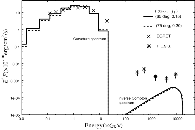
Figure 11: Pulsed gamma-ray spectrum from the Vela pulsar. The solid line and dotted line show the spectrum for $(\alpha_{inc},~{}j_{1})=(65^{\circ},0.15)$ and $(75^{\circ},0.2)$, respectively, with $(j_{2},j_{gap})=(0,0.1)$. The upper limits in 0.1-1TeV range has been determined by H.E.S.S. (Konopelko et al. 2005).

4.2 Comparison with the previous works

We have estimated the inclination angle that $\alpha_{inc}\geq 65$^∘ for the Vela pulsar. This result is marginally consistent with the result by RY95, in which $\alpha_{inc}\sim 65$^∘ for the Vela pulsar was predicted to explain the phase difference between the radio and $\gamma$-ray pulses. RY95 considered the gap having no external component ($j_{1}=j_{2}=0$) and starting from the conventional null surface. However, the present model has predicted the particle injection at the inner boundary ($j_{1}\neq 0,j_{2}=0$) to explain the observed flux, although the obtained inner boundary is located near the conventional null surface (Fig.9).

RY95 have assumed that the gap is extending to the light cylinder to produce the first peak of the light curves. In this paper, the gap geometry in Fig.9 that is favored for matching the spectrum of the Vela pulsar does not predict such long outer gap. However, we note that the accelerated particles in the outer gap emit the $\gamma$-ray photons outside the gap. As Fig.7 shows, the curvature photons emitted outside the gap by the outwardly moving particles also contribute to emissions above 100MeV. Specifically, the outwardly moving particles escape from the light cylinder with the Lorentz factor $\Gamma\sim 1.2\times 10^{7}(\Omega/100\mathrm{s^{-1}})^{-1/3}(<R_{c}>/\varpi_{lc})^{2/3}$, the corresponding curvature photon energy is $E^{lc}_{c}\sim 160(<R_{c}>/\varpi_{lc})$ MeV, where $<R_{c}>$ is the averaged curvature radius of the field line, along which the particles move. Therefore, although the outer boundary of the gap is located inside of the light cylinder, the high-energy photons are emitted near the light cylinder and the double peak structure in the calculated light curves is expected. The detail calculation will be done in the subsequent papers.

Dyks & Rudak (2003) proposed the radiation emission region starting from near the stellar surface to explain the presence of the outer-wing emissions and of the off-pulse emissions of the Crab pulsar. With the two-dimensional outer gap model, we found that such gap has a large particle injection at the outer boundary (Paper2). For such cases, $j_{1}\ll j_{2}$, however, the our model (e.g. $\mathrm{case}_{45}$ 4) also predicts the softer spectrum than the observed one of the Vela pulsar, as we discussed in §§3.3.

4.3 Screening of the electric field

As we have seen, the inner boundary, where $\tilde{E}_{||}=0$, is located at the position where the local charge density caused by the current is equal to the Goldreich-Julian charge density, that is, $(j_{1}-j_{2}+j_{g})\tilde{B}\sim\tilde{B_{z}}$ is satisfied on the inner boundary. However, the condition $|-(j_{1}-j_{2}+j_{g})\tilde{B}|<|-\tilde{B}_{z}|$ is satisfied between the stellar surface and the inner boundary. This negative charge depletion from the Goldreich-Julian charge density predicts a field-aligned electric field between the stellar surface, on which $\tilde{\Phi}_{nco}=0$ is defined, and the inner boundary. In such a case, there is a potential drop along the magnetic field lines. In the present paper, however, we have imposed the condition (37), $\tilde{\Phi}_{nco}=0$, at the inner boundary with the assumption that a screening mechanism of the electric field is working and that the potential drop between the stellar surface and the outer gap is much smaller than the potential drop in whole outer gap. In this subsection, therefore, we discuss the screening mechanism between the stellar surface and the inner boundary with the case that $j_{1}=j_{2}=0$.

Firstly, as the particles that screen the electric field, we mention a population of the electrons trapped between the stellar surface and the outer gap, such as the electron clouds trapped between the stellar surface and the boundary of the outer magnetospheric gap appeared in Smith, Michel & Thacker (2001). These electrons stabilize the force free surface (i.e. the inner boundary) between the plasma side and the outer gap side. Therefore, we expect that three kind of the particles will populate between the star and the inner boundary; the primary particles accelerated in the gap, the pair particles produced outside gap by the inwardly $\gamma$-rays and the trapped electrons. The vacuum outer gap model of CHR86 also assumed these trapped electrons between the stellar surface and the traditional null charge surface. Such trapped electrons will be distributed to fill the negative charge depletion, $j_{g}\tilde{B}-B_{z}$, from the Goldreich-Julian charge density, and to satisfy the condition $\tilde{E}_{||}=0$ between the stellar surface and the inner boundary.

Because the inner boundary will be affected by the plasma condition around the gap, we consider a particular case that there are no trapped electrons as an another possibility, that is, only primary and pair particles are migrating toward the stellar surface along the magnetic field line linking the star and the outer gap. With the assumption that the screening distance along the field line is much smaller than the trans-field thickness, we take the field-aligned part in the Poisson equation to obtain the field-aligned electric field. In this case, we can produce the solution that the field-aligned electric field $\tilde{E}_{||}$ undergoes spatial oscillation, and therefore is screened out by the small velocity difference of the pair particles. Because the amplitude of the potential ($\sim 10^{3}$ in the non-dimensional value) is much smaller than the potential drop ($\sim 10^{7}$) in the outer gap, the condition (37), $\tilde{\Phi}_{nco}=0$, at the inner boundary is a good treatment. Following Shibata, Miyazaki & Takahara (2002), however, we can show that a surprisingly large pair-creation rate is required to screen. In fact, the screening is achieved if the pairs were created with a rate

$$\left<\frac{dm}{ds_{||}}\right>\geq 0.0025\left(\frac{\Omega}{100\mathrm{rads^{-1}}}\right)\left(\frac{\gamma_{0}}{10^{3}}\right)^{2}\left(\frac{0.1\varpi_{lc}}{r}\right)~{}\mathrm{/cm},$$

where $m$ is the pair flux divided by $\Omega B_{in}/2\pi$, $B_{in}$ is the strength of the magnetic field at the inner boundary and $\gamma_{0}$ is the initial Lorentz factor of the pair. This rate indicates that the total number $N_{p}$ of the pairs produced within the typical screening distance $\sim 10^{5}$cm is $N_{p}/N_{GJ}\sim 10^{2}$, where $N_{GJ}$ represents the typical Goldreich-Julian value. Such a very large pair creation rate has not been predicted by the present cascade model, in which $dm/ds_{||}\sim 10^{-8}$ /cm (Fig.5). On these ground, we expect that the pair polarization does not screen out the field-aligned electric field within the small distance along the field line.

As discussed above, if no trapped electrons exist between the stellar surface and the outer gap, the field-aligned electric field will be caused outside the gap over a wide range along the field line. For such a case, the trans-field part in the Poisson equation determines the non-corotational potential, and the field-aligned part is not important, so that

$$\frac{\partial^{2}\tilde{\Phi}_{nco}}{\partial\xi_{\perp}^{2}}\sim-[-\tilde{\rho}_{0}+\tilde{\rho}_{+}+\tilde{\rho}_{-}],$$ (48)

where $\tilde{\rho}_{0}=j_{g}\tilde{B}-\tilde{B}_{z}$, $\tilde{\rho}_{+}$ and $\tilde{\rho}_{-}$ are, respectively, the charge densities of the par positrons and electrons, and $\xi_{\perp}$ is the distance in the trans-field direction. By ignoring the trans-field distribution of the charge density, the solution of equation (48) becomes $\tilde{\Phi}_{nco}\sim[-\tilde{\rho}_{0}+\tilde{\rho}_{+}+\tilde{\rho}_{-}]\xi_{\perp}(\tilde{D}_{\perp}-\xi_{\perp})/2$, where we use the boundary conditions that $\tilde{\Phi}_{nco}=0$ at $\xi_{\perp}=0$ and $\xi_{\perp}=\tilde{D}_{\perp}$, where $\tilde{D}_{\perp}$ represents the trans-field thickness. The field-aligned electric field is

$$\tilde{E}_{||}=\frac{\partial\tilde{\Phi}_{nco}}{\partial\xi_{||}}\sim\frac{\partial}{\partial\xi_{||}}(-\tilde{\rho_{0}}+\tilde{\rho}_{+}+\tilde{\rho}_{-})\frac{\xi_{\perp}(\tilde{D}_{\perp}-\xi_{\perp})}{2},$$ (49)

where $\xi_{||}$ is the field-aligned distance increasing toward the star.

Let us consider the sign of the field-aligned electric field of equation (49). If we ignore the contribution of the pair particles on the electric field, we find that the electric field becomes a positive because the outer gap is located on the field lines that curve away from the rotational axis and because the derivative $-\partial\tilde{\rho}_{0}/\partial{\xi_{||}}$ has a positive value between the stellar surface and the inner boundary. This positive electric field accelerates the pair electrons and decelerates the pair positrons, which are migrating toward the star. The continuity equations of the pair particles predict the field-aligned distribution of the charge density increasing toward the stellar surface, that is $\partial(\tilde{\rho}_{+}+\tilde{\rho}_{-})/\partial{\xi_{||}}>0$. The derivative of the total charge density in the right hand side of equation (49) has positive value, and therefore the effect of the pair polarization strengthens the positive electric field, which will appear unless there are such pair particles. Although some positrons are returned and are accelerated toward the gap by the positive electric field, the positive electric field will be held between the stellar surface and the inner boundary even if the effect of the discharge of the pairs is taken into account, as has been indicated by Hirotani (2005, in preparation).

Recently, Hirotani (2005) has solved the structure of the particular outer gap with the particle motion by setting the inner boundary at the stellar surface. He has indicated that such outer gap is composed of two region; one region (called ”minor part”) takes on a minor part of the potential drop of whole outer gap and has a small positive field-aligned electric field, and other (called ”major part”) takes on a major part of the potential drop and has a large field-aligned electric field. The major part, which corresponds to so-called outer gap in the present paper, is located in the outer magnetosphere and the minor part is extending between the stellar surface and the major part. Because the potential drop in the minor part of the gap is negligibly small in comparison with that in the major part, the boundary condition (37), $\Phi_{nco}=0$ (37), at the inner boundary of the major gap will be a good treatment as long as we are concerned with the major part of the gap.

With above discussions, therefore, we conclude that the boundary condition that $\tilde{\Phi}_{nco}=0$ at the inner boundary, where $\tilde{E}_{||}=0$, for the outer gap is a good treatment.

4.4 The connection between the global and local models

Figure 12: Outer gap structure with $(j_{1},j_{2})$=(0.1,0) and $\alpha_{inc}=65$^∘. Each panel is same with Fig.8. The solid lines show the results of the gap having the outer boundary located near the light cylinder at the lower part. The dashed lines show the results of the gap having the outer boundary of $\zeta_{out}=0.64.$

As we have seen, the outer gap structure and produced $\gamma$-ray spectrum are controlled by the current, which circulates in the magnetosphere globally. By comparing the observation, our local model can constrain the current flow pattern in the gap and the inclination angle, which cannot be observed directly. For further discussions, we would need a connection between the global and local models, as follows.

In the previous sections, we had considered the outer boundary following a curve line perpendicular to the magnetic field lines, that is $\zeta_{out}=$constant. It is notable that the shape of the outer boundary is controlled by the trans-field distribution of the total current.

Around the lower boundary, only a few pairs are produced by the pair creation, because the $\gamma$-rays are always emitted to the convex side of the magnetic field lines. Therefore, the shape of the outer boundary can become such as the gap structure displayed with solid lines in Fig.12, of which the outer boundary changes from $\zeta_{out}=0.64$ to $\zeta_{out}=1$ in region within 16% of gap thickness measured from the lower boundary. For comparison, we show the gap structure (dotted line) having the outer boundary of $\zeta_{out}=0.64$.

The electrons produced in the extending region emit the inwardly propagating $\gamma$-rays to convex side of the magnetic field lines and make pairs around the inner boundary. In the upper left panel of Fig.12, we can see that an effect of these new born pairs is the increase of the internal current around the hight $(\chi-\chi_{l})/(\chi_{up}-\chi_{l})\sim 0.2$ measured from the lower boundary. Fig.12. The difference between the two currents produces the difference between the outer boundaries in the upper right panel.

We find in Fig.12 that the calculated spectra for both cases are consistent with the observation. Therefore, it is difficult to deduce the shape of the outer boundary using the present local model. As a global study, CHR86 postulated that the outer gap is extending until the light cylinder, such as the gap geometry depicted with the solid line in Fig.12, due to the presence of an ionic (or a positronic) particle outflow from the light cylinder. For the aligned-rotator, on the other hand, Mestel et al. (1987) studied a structure of the magnetosphere with a global current and an acceleration region, which closes within the light cylinder (see also Mestel 1999). These global studies solve the global current, which interacts with the polar cap, the outer gap and the pulsar wind.

Because the local model can predict the current through the gap with the observations as we have seen in the present paper, and because the global study can solve the global current flow in the magnetosphere, the combination between the local and global studies would give a consistent understanding of the structure of the active pulsar magnetosphere. For such a discussion, a three-dimensional electrodynamical model is needed to compare with the observed phase-resolved spectra and light curves.

References

- Arons (1983) Arons J., 1983, ApJ, 266, 215
- Blumenthal (1970) Blumenthal G.R., Gould R.J., 1970, Rev. Mod. Phys., 42, 237
- Cha, Semback & Danks (1999) Cha A.N., Sembach K.R., Danks A.C. 1999, ApJ, 515L, 25
- Cheng, Ho & Ruderman (1986) Cheng K.S., Ho C., Ruderman M., 1986a, ApJ, 300, 500 (CHR86)
- Cheng, Ho & Ruderman (1986) Cheng K.S., Ho C., Ruderman M., 1986b, ApJ, 300, 522
- Cheng, Ruderman & Zhang (2000) Cheng K.S., Ruderman M., Zhang L., 2000, ApJ, 537, 964
- Daugherty & Harding (1996) Daugherty J.K., Harding A.K., 1996, ApJ, 458, 278
- Dyks & Rudak (2003) Dyks J., Rudak B., 2003, ApJ. 598, 1201
- Dyks, Harding & Rudak (2004) Dyks J., Harding A.K., Rudak B., 2004, ApJ, 606, 1125
- Fierro, Michelson, Nolan & Thompson (1998) Fierro J.M., Michelson P.F., Nolan P.L., Thompson D.J. 1998, ApJ, 494, 734
- Goldreich & Julian (1969) Goldreich P., Julian W.H., 1969, ApJ, 157, 869
- Harding, Strickman, Gwinn, Dodson, Moffet, & McCulloch (2002) Harding A.K., Strickman M.S., Gwinn C., Dodson R., Moffet D., McCulloch P., 2002, ApJ, 576, 376
- Hirotani (2005) Hirotani K., 2005, in preparation