The thermodynamics of collapsing molecular cloud cores using smoothed particle hydrodynamics with radiative transfer

Abstract

We present the results of a series of calculations studying the collapse of molecular cloud cores performed using a three-dimensional smoothed particle hydrodynamics code with radiative transfer in the flux-limited diffusion approximation. The opacities and specific heat capacities are identical for each calculation. However, we find that the temperature evolution during the simulations varies significantly when starting from different initial conditions. Even spherically-symmetric clouds with different initial densities show markedly different development. We conclude that simple barotropic equations of state like those used in some previous calculations provide at best a crude approximation to the thermal behaviour of the gas. Radiative transfer is necessary to obtain accurate temperatures.

1 Introduction

Radiative transfer is an important phenomena in star formation. Radiation sets the temperature of the gas during the collapse of a molecular cloud core. This both influences the degree of fragmentation of the cloud, and sets the minimum mass of brown dwarfs (the opacity limit for fragmentation; Low & Lynden-Bell, 1976). Once protostars have formed in a cloud, radiative and mechanical feedback from them can affect subsequent star formation. Such feedback mechanisms include protostellar jets and outflows from low-mass stars, and ionisation from massive stars which creates HII regions and destroys a cloud.

Computer simulations are vital in our efforts to understand the complex problem of star formation. Many previous simulations have used the smoothed particle hydrodynamics method (SPH) (e.g. Gingold & Monaghan, 1981; Pongracic et al., 1991; Bonnell et al., 1991; Nelson & Papaloizou, 1993; Bate et al., 1995; Klessen et al., 1998). Other methods used are typically based around grid-based codes (e.g. Larson, 1969; Boss & Bodenheimer, 1979; Boss & Myhill, 1992; Burkert & Bodenheimer, 1993; Truelove et al., 1997; Boss et al., 2000). SPH is a Lagrangian method first developed by Lucy (1977) and Gingold & Monaghan (1977) (see Monaghan, 1992, for a review). It approximates the fluid as a series of discrete fluid elements denoted by individual SPH particles and uses interpolation to obtain the fluid variables at any point in the simulation. SPH is conceptually simple to understand, and can naturally adapt its resolution to the local density distribution, unlike grid-based codes which require complex adaptive-mesh refinement algorithms to perform the same task. This property makes it ideal for use in star formation, where densities may range over many orders of magnitude in a single simulation.

Despite these advantages, few attempts have been made to include radiative transfer into SPH (Lucy, 1977; Brookshaw, 1985, 1986; Oxley & Woolfson, 2003; Whitehouse & Bate, 2004), and until recently (Bastien, Cha & Viau, 2004, 2005) SPH with radiative transfer has not been applied to star formation. Instead, many past simulations have simply used isothermal or barotropic equations of state to model the collapse of a molecular cloud. The former is only valid up to densities of $\sim 10^{-13}$ g cm^-3 at which point the cloud traps radiation efficiently enough for the cloud to begin to heat up. The latter is usually based on the evolution of the temperature at the highest density during the collapse of spherically symmetric clouds as calculated using radiative transfer (e.g. Larson, 1969; Winkler & Newman, 1980; Masunaga & Inutsuka, 2000). However, a barotropic equation of state can at best only hope to provide an adequate description of temperature at the density maximum; it is unlikely to give an accurate temperature distribution during a three-dimensional calculation with complex density and velocity structure. Indeed, Boss et al. (2000) performed grid-based calculations of the collapse of a molecular cloud core both with a barotropic equation of state and with radiative transfer in the Eddington approximation and found they differed somewhat. However, they did not examine in detail how the relation between temperature and density differed from that of the barotropic equation of state spatially and temporally, or its dependence on initial conditions.

Whitehouse, Bate & Monaghan (2005) recently presented an implicit algorithm for calculating radiative transfer using the flux-limited diffusion approximation within the SPH formalism. This paper describes a three-dimensional implementation of this algorithm and uses it to examine the thermodynamics during the collapse of molecular cloud cores. Section 2 describes the changes necessary to the radiative transfer algorithm of Whitehouse et al. (2005) for use in three dimensions and the initial conditions for our star formation calculations. Section 3 presents the results of simulations of the collapse of molecular cloud cores with different initial conditions and examines the evolution of their temperature structure. Finally, section 4 summarises the main conclusions of this paper.

2 Method and initial conditions

The code used in this paper is based on that of Bate (Bate, 1995; Bate et al., 1995), which originated from that of Benz (Benz, 1990; Benz et al., 1990). The code includes individual timesteps, and uses a tree to calculate self-gravity. The smoothing lengths of particles are variable in time and space, subject to the constraint that the number of neighbours for each particle must remain approximately constant at $N_{\rm neigh}=50$. We use the standard form of artificial viscosity (Monaghan & Gingold 1983; Monaghan 1992) with strength parameters $\alpha_{\rm{}_{v}}=1$ and $\beta_{\rm v}=2$. To perform radiation transport, the algorithm from Whitehouse et al. (2005), adapted for use in three dimensions, was added. The code has been parallelised by M. Bate using OpenMP.

2.1 Three-dimensional flux-limited diffusion

In a frame co-moving with the fluid, and assuming local thermal equilibrium (LTE), the equations governing the time-evolution of radiation hydrodynamics (RHD), integrated over frequency, are

$$\frac{D\rho}{Dt}+\rho\mbox{\boldmath$\nabla\cdot v$}=0~{},$$ (1)

$$\rho\frac{D\mbox{\boldmath$v$}}{Dt}=-\nabla p+\frac{\mbox{$\kappa\rho$}}{c}\mbox{\boldmath$F$}~{},$$ (2)

$$\rho\frac{D}{Dt}\left(\frac{E}{\rho}\right)=-\mbox{\boldmath$\nabla\cdot F$}-\mbox{\boldmath$\nabla v${\bf:P}}+4\pi\kappa\rho B-c\kappa\rho E~{},$$ (3)

$$\rho\frac{D}{Dt}\left(\frac{e}{\rho}\right)=-p\mbox{\boldmath$\nabla\cdot v$}-4\pi\kappa\rho B+c\kappa\rho E~{},$$ (4)

$$\frac{\rho}{c^{2}}\frac{D}{Dt}\left(\frac{\mbox{\boldmath$F$}}{\rho}\right)=-\mbox{\boldmath$\nabla\cdot${\bf P}}-\frac{\mbox{$\kappa\rho$}}{c}\mbox{\boldmath$F$}~{}$$ (5)

(Mihalas & Mihalas, 1984; Turner & Stone, 2001). In these equations, $D/Dt\equiv\partial/\partial t+\mbox{\boldmath$v\cdot\nabla$}$ is the convective derivative. The symbols $\rho$, $e$, $v$ and $p$ represent the material mass density, energy density, velocity, and scalar isotropic pressure respectively. The total frequency-integrated radiation energy density, momentum density (flux) and pressure tensor are represented by $E$, $F$, and P, respectively. In this paper, we use a grey opacity, $\kappa$ (i.e., it is independent of frequency).

To solve radiation transport within SPH, we evolve both the specific internal energy of the gas $u$, and the specific radiation energy $\xi=E/\rho$ implicitly using the algorithm of Whitehouse et al. (2005). The principle difference between the one-dimensional and three-dimensional forms of the radiative transfer equations is the radiation pressure term (the second term on the right-hand side of equation 3). In one-dimension this term can be written using the divergence of the gas velocity. However, in three dimensions this becomes the tensor product $\nabla v$:P, where the Eddington pressure tensor P is given by

$$\mbox{\bf P}=\mbox{\boldmath$f$}E.$$ (6)

The components of the Eddington tensor $f$ are given by

$$\mbox{\boldmath$f$}=\frac{1}{2}\left(1-f\right)\mbox{\boldmath$I$}+\frac{1}{2}\left(3f-1\right)\mbox{\boldmath$\hat{n}$}\mbox{\boldmath$\hat{n}$}.$$ (7)

Here $f$ is the dimensionless scalar Eddington factor, and $\hat{n}$ is the unit vector in the direction of the energy density gradient $\nabla E/|\nabla E|$. For example, in Cartesian coordinates, the first component of the tensor is given by

$$\frac{1}{2}(1-f)+\frac{\frac{1}{2}(3f-1)\left(\frac{\partial E}{\partial x}\right)^{2}}{|\nabla E|^{2}}~{}\xi,$$ (8)

and the next by

$$\frac{\frac{1}{2}(3f-1)\left(\frac{\partial E}{\partial x}\right)\left(\frac{\partial E}{\partial y}\right)}{|\nabla E|^{2}}~{}\xi,$$ (9)

and so on.

The scalar Eddington factor $f$ is related to the flux-limiter $\lambda$, by the expression

$$f=\lambda+\lambda^{2}R^{2},$$ (10)

where $R=|\nabla E|/(\kappa\rho E)$. In this paper, we choose the flux limiter of Levermore & Pomraning (1981)

$$\lambda(R)=\frac{2+R}{6+3R+R^{2}}.$$ (11)

In the optically thick limit, $R\rightarrow 0$, $\lambda\rightarrow 1/3$, and P becomes isotropic.

2.2 Specific heat capacity and opacity

The above equations are closed by the application of an equation of state for the gas. We use the ideal gas equation of state

$$p=\frac{R_{\rm g}}{\mu}\rho T_{\rm g},$$ (12)

where $R_{\rm g}$ is the gas constant, $\mu$ is the mean molecular mass and the gas temperature is $T_{\rm g}=u/c_{\rm v}$. The temperature of the radiation is given by $T_{\rm r}=(E/a)^{1/4}$.

We use the specific heat capacity $c_{\rm v}$ of Black & Bodenheimer (1975), which accounts for the dissociation of molecular hydrogen, and the ionization of both hydrogen and helium. It omits any contribution due to metals.

$$c_{\rm v}= \displaystyle X\left(1-y\right)E(H_{2})+\left[1.5X\left(1+x\right)y+0.375Y\left(1+z_{\rm 1}+z_{\rm 1}z_{\rm 2}\right)\right]R_{\rm g}$$ (13)

$$+X\left(1.304\times 10^{13}x+2.143\times 10^{12}\right)y/T_{\rm g}+$$

$$\displaystyle Y\left(5.888\times 10^{12}\left(1-z_{\rm 2}\right)+1.892\times 10^{13}z_{\rm 2}\right)z_{\rm 1}/T_{\rm g},$$

where $X$ and $Y$ are the mass fractions of hydrogen and helium respectively (in the simulations presented in this paper, $X=0.70$ and $Y=0.28$), $y$ is the dissociation fraction of hydrogen, $x$ the ionisation fraction of hydrogen, and $z_{\rm 1}$ and $z_{\rm 2}$ are the degrees of single and double ionisation of helium, respectively. $E(H_{\rm 2})$ gives the contribution to the specific heat capacity from molecular hydrogen (Black & Bodenheimer, 1975). The ionisation fractions are calculated using the Saha equation.

The variation in mean molecular mass $\mu$ with temperature was also taken from Black & Bodenheimer (1975) to be

$$\mu^{-1}=\left[2X\left(1+y+2xy\right)+Y\left(1+z_{\rm 1}+z_{\rm 1}z_{\rm 2}\right)\right]/4.$$ (14)

The opacity table from Alexander (1975) (the fourth King model) was used for the gas opacity and Pollack, McKay & Christofferson (1985) for the dust opacity. The opacity values were stored in a table containing the opacity at various temperatures and densities up to 10,000 K and 1 g cm^-3 respectively, and bilinear interpolation in log-space was used to get the required value. Above 10,000 K, the opacity was taken to be the lesser of extrapolating from the last two points in the table, or Kramer’s opacity

$$\kappa_{\rm K}=1.2512\times 10^{22}\rho T^{-\frac{7}{2}},$$ (15)

until the electron scattering opacity $\kappa_{\rm es}=0.4~{}$cm² g^-1 becomes the dominating opacity source at very high temperatures.

For temperatures above a few million K, the opacity, specific heat capacity and mean molecular mass become constant because the contribution of metals is neglected. These three quantities were updated during every iteration of the implicit scheme.

2.3 Initial conditions

The simulations described in this paper used three different sets of initial conditions. The first was the spherically symmetric collapse of Boss & Myhill (1992). They began with a $1.2~{}{\rm M}_{\odot}$ sphere of uniform density $\rho=1.7\times 10^{-19}$ g cm^-3, giving a free-fall time of $t_{\rm ff}=1.61\times 10^{5}$ years. The cloud radius was $1.5\times 10^{17}$ cm, and the initial temperature of both the gas and the radiation field was $10$ K.

The other two initial conditions were based on those of Boss & Bodenheimer (1979). They began with a $1.0~{}{\rm M}_{\odot}$ sphere of density $\rho=1.44\times 10^{-17}$ g cm^-3 and radius $3.2\times 10^{16}$ cm, giving a free-fall time of $t_{\rm ff}=1.75\times 10^{4}$ years. Their cloud was initially in solid-body rotation with an angular velocity of $1.6\times 10^{-12}$ rad s^-1. Superimposed on the underlying density was an $m=2$ density perturbation satisfying

$$\rho=\rho_{0}[1+0.5\cos(m\phi)]$$ (16)

where $\phi$ is the angle in the plane perpendicular to the axis of rotation. The ratio of thermal energy to magnitude of the gravitational energy was initially 0.26 and the ratio of rotational energy to the magnitude of the gravitational energy was 0.20. Using our equation of state, the initial temperature of the gas and radiation were therefore set to 12 K. We performed calculations with initial conditions identical to those of Boss & Bodenheimer (1979), and also a spherically symmetric version in which there was no $m=2$ density perturbation applied and the cloud was not rotating.

We performed simulations with 5000, 50,000, 150,000 and 500,000 particles. Of these, simulations with 50,000 particles and greater resolve the Jeans mass according to the criteria set out in Bate & Burkert (1997). The calculations were performed on the United Kingdom Astrophysical Fluids Facility (UKAFF). The highest resolution (500,000 particle) calculation took a total of approximately 3000 CPU hours (running across multiple processors).

3 Results

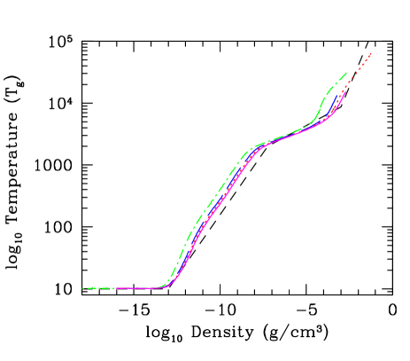
Figure 1: We show the evolution of the maximum temperature and density during the calculations that start from the initial conditions of Boss & Myhill (1992) for different resolutions. The calculations were performed using 5000 (dot-dashed green line), 50,000 (long-dashed blue line), 150,000 (dotted red line) and 500,000 (solid magenta line) particles. The results converge as the resolution is increased, with 50,000 or greater numbers of particles required to achieve reasonable results. For comparison, the short-dashed line gives the temperature-density relation of the barotropic equation of state used by Bate (1998).

A brief summary of the expected behaviour during a spherically symmetric collapse is as follows (see Bodenheimer & Sweigart, 1968; Larson, 1969, for more details). A Jeans-unstable uniform cloud of molecular gas will begin to collapse under its own self-gravity. The collapse occurs such that the density in the outer parts of the cloud falls off with radius $r$ as $\rho\propto r^{-2}$, while the uniform-density inner part of the cloud collapses to higher and higher densities but contains a decreasing fraction of the mass as the collapse proceeds. Initially, the collapse is isothermal, as the material is optically thin. However, once the central region reaches a critical density ($\sim 10^{-13}$ g cm^-3) it becomes optically thick and starts to heat as energy can no longer be radiated away. The central temperature and density both rise rapidly, until thermal pressure can counter the collapse. This results in the formation of a pressure-supported core in the centre of the cloud. Mass continues to infall onto this core, increasing its mass and temperature. While at low temperatures, the molecular hydrogen behaves like a monatomic gas (the ratio of specific heats $\gamma=5/3$). However, when the temperature approaches $\sim 100$ K (at densities $\sim 10^{-11}$ g cm^-3) additional degrees of freedom become available and $\gamma=7/5$. This phenomenon which is included in our specific heat capacity is not typically included in the simple barotropic equation of state. Once the core reaches $\sim 2000$ K, the molecular hydrogen begins to dissociate. As energy is diverted into this dissociation rather than thermal support, the core begins a second collapse phase. Once the hydrogen has been fully dissociated, it forms a second (“stellar”) core, once again supported by thermal pressure. This core continues to increase mass and temperature as material falls onto it from the envelope.

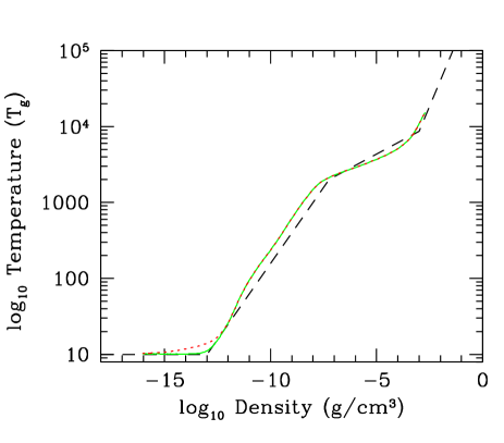
Figure 2: We show the evolution of the maximum gas (solid green line) and radiation (dotted red line) temperatures at the maximum density during the Boss & Myhill (1992) calculation. This was our highest resolution (500,000 particles) calculation. The gas and radiation temperatures are identical except during the transition from optically thin to optically thick. For comparison, the short-dashed line gives the temperature-density relation of the barotropic equation of state used by Bate (1998).

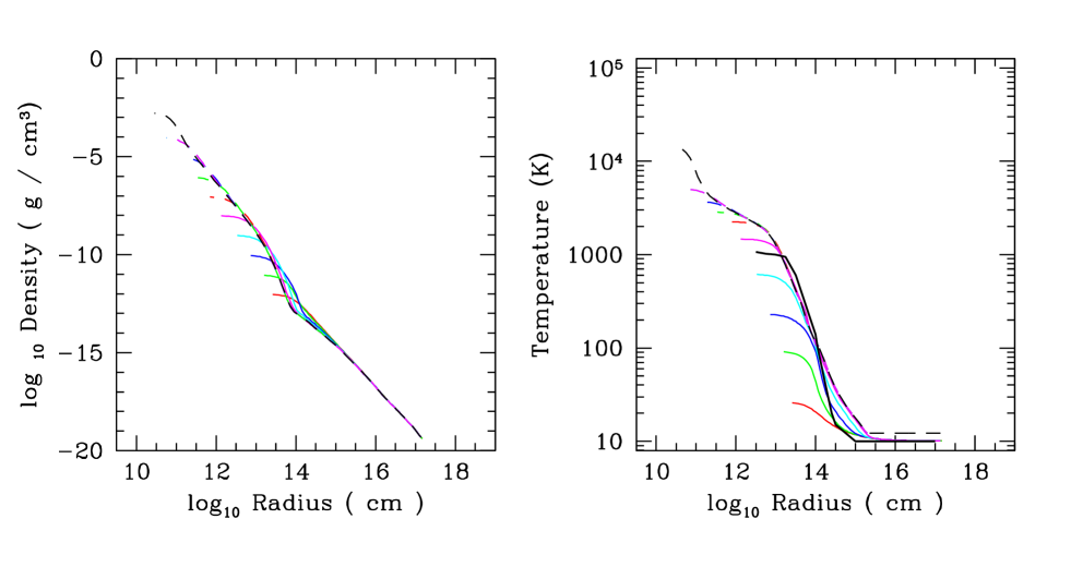
Figure 3: Radial profiles of density (left panel) and gas temperature (right panel) at various stages during the highest resolution (500,000 particles) Boss & Myhill (1992) calculation. A profile is plotted every order of magnitude in maximum density from $10^{-12}$ to $10^{-3}$ g cm^-3 and finally at $2\times 10^{-3}$ g cm^-3. For comparison, the thick solid black lines give the profiles from Boss & Myhill (1992) when the temperature in their calculation was $\approx 1000$ K.

We present results showing the evolution with time of our calculations in Figures 1 to 8. The short-dashed black line in these figures is the barotropic equation of state used by Bate (1998), given for comparison. Unless otherwise stated, we plot the temperature of the gas rather than that of the radiation field.

As far as we are aware, these are the first three-dimensional radiative transfer calculations to follow the collapse of a molecular cloud core beyond the formation of the first pressure-supported core and the dissociation of molecular hydrogen to the formation of the stellar core. Boss (1984) performed one- and two-dimensional radiative transfer calculations that followed the collapse of a molecular cloud core well beyond the formation of the first pressure-supported core. However, in order to accomplish this he had to employ several numerical artifices, begging the question of how we are able to perform three-dimensional calculations. Boss’ first artifice was to implement two regions of his grid that were evolved using different timesteps in order to follow the first core over many dynamical times using short timesteps but simultaeously model the envelope with larger timesteps. He also damped out oscillations of the first core to decrease the amount of computational effort required. In our calculations, we encountered no difficulties in modelling the cloud collapse through the first core phase and onto the formation of the stellar core. We believe there are three reasons for this. First, our code employs individual timesteps (Bate, 1995; Bate et al., 1995) for each particle (i.e. similar to, but even more efficient than, the way Boss evolved his calculation in with two spatially distinct timesteps). By the end of our highest resolution calculation, some particles within the stellar core were being evolved using timesteps of less than 1/40 of a second ($\approx 10^{5}$ times smaller than those in the outer parts of the cloud). Second, our calculations used the standard form of SPH viscosity with none of the possible viscosity-reducing formulations. In each calculation, the first core undergoes oscillations after its formation, as observed in earlier work, but the viscosity likely damped these oscillations in a similar way to Boss’ artifice. Finally, in the twenty years between Boss’ and our calculations, computers have become very much quicker.

3.1 Results using Boss and Myhill initial conditions

Figure 1 shows the evolution of maximum temperature and density during the Boss & Myhill (1992) collapse calculations. We performed the collapse with four different resolutions. With 5000 particles (green line) the cloud heats at an earlier stage than in the higher resolution simulations, presumably due to insufficient resolution. The 50,000 particle collapse (blue) is much cooler for a given maximum density, while the two highest resolution simulations appear to be converging towards a single curve. We conclude that 50,000 to 150,000 particles (i.e. approximately the same number as required to resolve the Jeans mass) are sufficient to model the thermal behaviour reasonably accurately. The evolution of maximum temperature and density follows the barotropic equation of state (dashed line) in a qualitative sense, but there are still differences in temperature of up to $\approx 50$ percent between the radiative transfer and the barotropic equation of state at various stages during the collapse.

Figure 2 shows the evolution of both the gas temperature (green) and the radiation temperature (red) for the highest resolution (500,000 particles) Boss & Myhill (1992) collapse. The radiation temperature is equal to the gas temperature at most stages, except in the vicinity of the transition between the optically thin and thick regimes. This can be seen in the figure from densities of $\sim 10^{-15}$ to $10^{-12}$ g cm^-3 when the cloud initially begins to heat. Here the radiation temperature is up to a factor of two greater than that of the gas. Later in the calculation, gas that is optically thick has the same temperature as the radiation and the two remained coupled as the gas collapses to very high densities. However, there is always a region where the gas transitions from optically thin to optically thick where the temperatures differ.

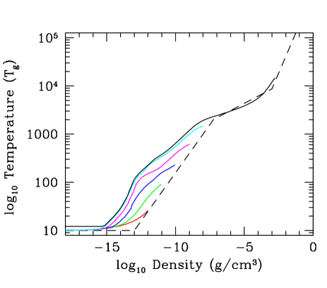
Figure 4: Snapshots of temperature versus density at various stages during the highest resolution (500,000 particles) Boss & Myhill (1992) collapse. A snapshot is plotted every order of magnitude in maximum density from $10^{-12}$ to $10^{-8}$ g cm^-3 and finally at $2\times 10^{-3}$ g cm^-3. Note that at late times the temperature differs by more than an order of magnitude from that given by the barotropic equation of state (dashed line).

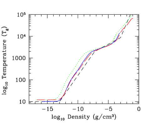
Figure 5: The evolution the maximum temperature and density during calculations starting from three different sets of initial conditions. The three calculations are the spherically-symmetric (dotted green line) and $m=2$ rotating (long-dashed red line) Boss & Bodenheimer (1979) collapses and the spherically-symmetric Boss & Myhill (1992) collapse (solid blue line). All calculations were performed using 50,000 particles. Note that different initial conditions can lead to very different temperature evolution. For comparison, the short-dashed line gives the temperature-density relation of the barotropic equation of state used by Bate (1998).

Figure 3 shows density (left) and gas temperature (right) plotted against radius as the collapse passes various values of the maximum density. The first core can be seen at a radius of $\sim 10^{14}$ cm where the density and temperature gradients change abruptly. Similarly, the transition to the stellar core can be seen at a radius of $\sim 10^{12}$ cm. Boss & Myhill (1992) give the density and temperature profiles when the central temperature reaches $\approx 1000$ K. We reproduce their profiles as the thick solid black lines in Figure 3. Our results are in good agreement with theirs, the main difference being that our results give slightly higher temperatures at radii $\sim 10^{15}$ cm, presumably due to the fact that we use flux-limited diffusion while Boss & Myhill (1992) use the Eddington approximation (the former retards radiation transport near the surface of the first core).

In Figure 4, we plot temperature versus density at a series of snapshots during the highest resolution calculation (since both temperature and density are monotonically decreasing functions of radius, we can plot these as lines for each snapshot). The figure clearly shows that even if it were possible to construct a barotropic equation of state to follow the evolution of maximum density and temperature, it would generally underestimate the temperature of the gas away from the maximum. In the figure, the barotropic equation underestimates the temperature by more than an order of magnitude at densities $\sim 10^{-13}$ g cm^-3 at late times.

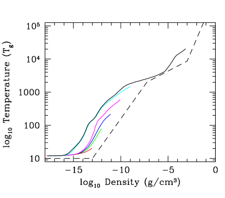
Figure 6: Snapshots of temperature versus density at various stages during the 50,000 particle spherically-symmetric Boss & Bodenheimer (1979) calculation. A snapshot is plotted every order of magnitude in maximum density from $10^{-13}$ to $10^{-9}$ g cm^-3 and finally at $10^{-3}$ g cm^-3. As with the Boss & Myhill (1992) initial conditions, the temperature differs by more than an order of magnitude from that given by the barotropic equation of state (dashed line) at late times.

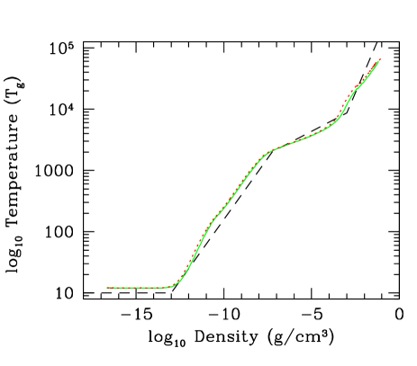
Figure 7: The evolution of the maximum temperature and density during the calculations that start from the initial conditions of Boss & Bodenheimer (1979), including the $m=2$ density perturbation and rotation, for two different resolutions. The calculations were performed using 50,000 (dotted red line) and 150,000 (solid green line) particles. The two resolutions give similar results. For comparison, the dashed line gives the temperature-density relation of the barotropic equation of state used by Bate (1998).

3.2 Results using spherically symmetric Boss and Bodenheimer initial conditions

Figure 5 shows the evolution of the maximum value of temperature and density for the three types of initial conditions, each performed with 50,000 particles. The spherically-symmetric Boss & Bodenheimer (1979) collapse (green line) begins to heat at a much lower density than the Boss & Myhill (1992) collapse (blue). Essentially the only difference between these calculations is the initial density of the two clouds, the former is initially almost two orders of magnitude denser, and yet the temperature evolutions are quite different. Figure 6 shows that, as with the Boss & Myhill (1992) collapse, the spatial and temporal evolution of the temperature is also complex. Again, these results demonstrate that a barotropic equation of state cannot accurately describe the temperature distribution during such cloud collapses.

3.3 Binary star formation

The result of the Boss & Bodenheimer (1979) initial conditions, including the $m=2$ density perturbation and rotation, is to form a wide binary with a separation of $\approx 1000$ AU (Bate et al., 1995). Using these initial conditions, the evolution of the maximum temperature versus density is much cooler than that from its spherically-symmetric counterpart (see Figure 5, red line). In fact, coincidentally, it is actually quite close to the evolution obtained with the Boss & Myhill (1992) initial conditions. There are likely to be two reasons for the cooler temperatures at the same maximum density in the rotating collapse. First, the collapse to form the stars is delayed by the rotational support (they form at $t=1.30$ initial cloud free-fall times instead of just over one free-fall time for the spherically symmetric case). The slower collapse allows more time for energy to be radiated away from the object. Second, the presence of rotation means that the distribution of material around each of the collapsed objects is no longer spherically symmetric. In particular, there are low density cavities along the rotation axes and high densities in the discs. Radiation can more easily escape through these cavities than in the spherically symmetric case.

We also tested the effect of resolution on the Boss & Bodenheimer (1979) binary star initial conditions, using 50,000 and 150,000 particles (Figure 7, red and green lines respectively). As with the Boss & Myhill (1992) initial conditions, increasing the resolution above 50,000 particles has little effect on the temperature evolution showing that the calculations are essentially converged.

The difference in evolution between the radiation and the gas temperatures is shown in Figure 8, in a manner similar to Figure 2. Again the only significant difference occurs during the transition from the optically thin to optically thick regimes at densities around $10^{-15}$ to $10^{-12}$ g cm^-3.

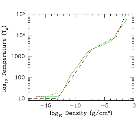
Figure 8: The evolution of the maximum gas (solid green line) and radiation (dotted red line) temperatures at the maximum density during the Boss & Bodenheimer (1979) calculation, including the initial $m=2$ density perturbation and rotation. The calculation was performed using 150,000 particles. The gas and radiation temperatures are identical except during the transition from optically thin to optically thick. For comparison, the dashed line gives the temperature-density relation of the barotropic equation of state used by Bate (1998).

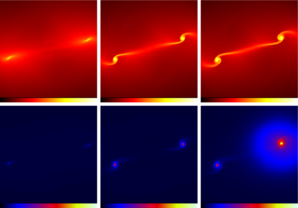
Figure 9: Snapshots of the logarithmic column density, $N$, (upper panels) and mass-weighted gas temperature, $T_{\rm g}$, (lower panels) parallel to the rotation axis for the 150,000 particle Boss & Bodenheimer (1979) calculation, including the initial $m=2$ density perturbation and rotation. The density scale covers $-1<\log N<3.5$ with N measured in g cm^-2 while the temperature scale ranges from $1<\log T_{\rm g}<3$. The snapshots are given when the maximum densities are $10^{-12}$, $10^{-10}$, and $10^{-1}$ g cm^-3. The corresponding times are $1.18$, $1.24$ and $1.30$ initial cloud free-fall times. The molecular cloud core collapses to form a protostellar binary system. Note that the dense gas within the spiral arms is cooler than the surfaces of arms (e.g., lower middle panel and the left-hand object in the lower right panel). In the lower right panel, the protostar on the right has formed a stellar core and thus heated the surrounding gas significantly more than the protostar on the left. At the time plottted, the left protostar has not quite undergone molecular hydrogen dissociation to form a stellar core. The two objects form stellar cores at slightly different times because of small asymmetries in the initial conditions.

4 Conclusions

The results of our study show that the initial conditions in a molecular cloud core such as the density and velocity configurations have a large effect on the evolution of the temperature as the cloud collapses. The evolution of the maximum temperature and density during the collapse cannot be approximated by a single barotropic equation of state. Furthermore, even if a satisfactory description of this evolution was able to be formulated by a simple equation of state, it would do a very poor job of setting the temperature away from the location of the density maximum. We find the barotropic equation of state used in many previous simulations (e.g. Bate, 1998) may underestimate the temperature by up to a factor of two to three for the density maximum, and by more than an order of magnitude in other parts of the cloud. In principle, this may seriously affect the evolution of a molecular cloud core, even altering how it fragments since the Jeans mass scales with gas temperature as $T_{\rm g}^{3/2}$. Therefore, if possible, radiative transfer should be used.

References

- Alexander (1975) Alexander D. R., 1975, ApJS, 29, 363
- Bastien et al. (2004) Bastien P., Cha S.-H., Viau S., 2004, in Revista Mexicana de Astronomia y Astrofisica Conference Series SPH with radiative transfer: method and applications. pp 144–147
- Bastien et al. (2005) Bastien P., Cha S.-H., Viau S., 2005, ApJ, submitted
- Bate (1995) Bate M., 1995, Ph.D. Thesis, University of Cambridge
- Bate (1998) Bate M. R., 1998, ApJL, 508, L95
- Bate et al. (1995) Bate M. R., Bonnell I. A., Price N. M., 1995, MNRAS, 277, 362
- Bate & Burkert (1997) Bate M. R., Burkert A., 1997, MNRAS, 288, 1060
- Benz (1990) Benz W., 1990, The Numerical Modeling of Nonlinear Stellar Pulsations: Problems and Prospects, ed. Buchlet, J. R., Kluwer Academic Publishers, Dordrecht., 269
- Benz et al. (1990) Benz W., Cameron A. G. W., Press W. H., Bowers R. L., 1990, ApJ, 348, 647
- Black & Bodenheimer (1975) Black D. C., Bodenheimer P., 1975, Ap. J, 199, 619
- Bodenheimer & Sweigart (1968) Bodenheimer P., Sweigart A., 1968, ApJ, 152, 515
- Bonnell et al. (1991) Bonnell I., Martel H., Bastien P., Arcoragi J.-P., Benz W., 1991, ApJ, 377, 553
- Boss (1984) Boss A. P., 1984, ApJ, 277, 768
- Boss & Bodenheimer (1979) Boss A. P., Bodenheimer P., 1979, ApJ, 234, 289
- Boss et al. (2000) Boss A. P., Fisher R. T., Klein R. I., McKee C. F., 2000, ApJ, 528, 325
- Boss & Myhill (1992) Boss A. P., Myhill E. A., 1992, ApJS, 83, 311
- Brookshaw (1985) Brookshaw L., 1985, Proceedings of the Astronomical Society of Australia, 6, 207
- Brookshaw (1986) Brookshaw L., 1986, Proceedings of the Astronomical Society of Australia, 6, 461
- Burkert & Bodenheimer (1993) Burkert A., Bodenheimer P., 1993, MNRAS, 264, 798
- Gingold & Monaghan (1977) Gingold R. A., Monaghan J. J., 1977, MNRAS, 181, 375
- Gingold & Monaghan (1981) Gingold R. A., Monaghan J. J., 1981, MNRAS, 197, 461
- Klessen et al. (1998) Klessen R. S., Burkert A., Bate M. R., 1998, ApJL, 501, L205+
- Larson (1969) Larson R. B., 1969, MNRAS, 145, 271
- Levermore & Pomraning (1981) Levermore C. D., Pomraning G. C., 1981, ApJ, 248, 321
- Low & Lynden-Bell (1976) Low C., Lynden-Bell D., 1976, MNRAS, 176, 367
- Lucy (1977) Lucy L. B., 1977, AJ, 82, 1013
- Masunaga & Inutsuka (2000) Masunaga H., Inutsuka S.-i., 2000, ApJ, 531, 350
- Mihalas & Mihalas (1984) Mihalas D., Mihalas B. W., 1984, Foundations of Radiation Hydrodynamics. Oxford University Press
- Monaghan (1992) Monaghan J. J., 1992, Ann. Rev. Astron. Astrophys., 30, 543
- Nelson & Papaloizou (1993) Nelson R. P., Papaloizou J. C. B., 1993, MNRAS, 265, 905
- Oxley & Woolfson (2003) Oxley S., Woolfson M. M., 2003, MNRAS, 343, 900
- Pollack et al. (1985) Pollack J. B., McKay C. P., Christofferson B. M., 1985, Icarus, 64, 471
- Pongracic et al. (1991) Pongracic H., Chapman S., Davies R., Nelson A., Disney M., Whitworth A., 1991, Memorie della Societa Astronomica Italiana, 62, 851
- Truelove et al. (1997) Truelove J. K., Klein R. I., McKee C. F., Holliman J. H., Howell L. H., Greenough J. A., 1997, ApJL, 489, L179+
- Turner & Stone (2001) Turner N. J., Stone J. M., 2001, ApJS, 135, 95
- Whitehouse & Bate (2004) Whitehouse S. C., Bate M. R., 2004, MNRAS, 353, 1078
- Whitehouse et al. (2005) Whitehouse S. C., Bate M. R., Monaghan J. J., 2005, MNRAS, accepted
- Winkler & Newman (1980) Winkler K.-H. A., Newman M. J., 1980, ApJ, 238, 311