The Las Campanas/AAT Rich Cluster Survey – III.
Spectroscopic Studies of X-ray Bright Galaxy Clusters at $z\sim 0.1$

Abstract

We present the analysis of the spectroscopic and photometric catalogues of 11 X-ray luminous clusters at $0.07<z<0.16$ from the Las Campanas / Anglo-Australian Telescope Rich Cluster Survey. Our spectroscopic dataset consists of over 1600 galaxy cluster members, of which two thirds are outside $r_{200}$. These spectra allow us to assign cluster membership using a detailed mass model and expand on our previous work on the cluster colour-magnitude relation where membership was inferred statistically. We confirm that the modal colours of galaxies on the colour magnitude relation become progressively bluer with increasing radius $d(B-R)/dr_{p}=-0.011\pm 0.003$ and with decreasing local galaxy density $d(B-R)/dlog(\Sigma)=-0.062\pm 0.009$. Interpreted as an age effect, we hypothesize that these trends in galaxy colour should be reflected in mean H$\delta$ equivalent width. We confirm that passive galaxies in the cluster increase in H$\delta$ line strength as $d$H$\delta/dr_{p}=0.35\pm 0.06$. Therefore those galaxies in the cluster outskirts may have younger luminosity-weighted stellar populations; up to 3 Gyr younger than those in the cluster centre assuming $d(B-R)/dt=0.03$ mag per Gyr (Kodama & Arimoto 1997). A variation of star formation rate, as measured by [Oii]$\lambda 3727\rm{\AA}$, with increasing local density of the environment is discernible and is shown to be in broad agreement with previous studies from the 2dF Galaxy Redshift Survey and the Sloan Digital Sky Survey. We divide our spectra into a variety of types based upon the MORPHs classification scheme. We find that clusters at $z\sim 0.1$ are less active than their higher redshift analogues: about 60 per cent of the cluster galaxy population is nonstarforming, with a further 20 per cent in the post-starburst class and 20 per cent in the currently active class, demonstrating that evolution is visible within the past 2–3 Gyr. We also investigate unusual populations of blue and very red nonstarforming galaxies and we suggest that the former are likely to be the progenitors of galaxies which will lie on the colour-magnitude relation, while the colours of the latter possibly reflect dust reddening. We show that the cluster galaxies at large radii consist of both backsplash ones and those that are infalling to the cluster for the first time. We make a comparison to the field population at $z\sim 0.1$ and examine the broad differences between the two populations. Individually, the clusters show significant variation in their galaxy populations which we suggest reflects their recent infall histories.

1 Introduction

Clusters of galaxies represent an ideal cosmological laboratory. They allow the study of large numbers of galaxies ($\sim 10^{3}$), all at common distances. Since they are visible out to high redshifts, they are also excellent tools for studying galaxy evolution and the role that environment plays in this evolution. Indeed, the environment of a galaxy is likely to be one of the most important factors that affect its star formation rate (Osterbrock 1960; Dressler, Thompson & Shectman 1985; Abraham et al. 1996; Balogh et al. 1997; Balogh et al. 1998; Smail et al. 1998; Poggianti et al. 1999; Kodama et al. 2001; Lewis et al. 2002; Pimbblet et al. 2002 [P02 herein]; Gómez et al. 2003; Balogh et al. 2004). However, it could also be that initial conditions are just as important as environment in determining the star formation history of galaxies.

It is well-established that galaxies that reside in the high density cores of clusters generally exhibit lower current star formation rates than equivalent field galaxies. The morphology-density relationship ($T-\Sigma$; Dressler 1980; Whitmore, Gilmore & Jones 1993; Dressler et al. 1997; Smith et al. 2005; see also Oemler 1974) can explain some of this trend. Broadly, it shows that late-type galaxies, which are expected to correspond to star-forming systems, preferentially occupy low-density regions whilst conversely, early-type passive galaxies tend to be situated in regions of high density such as at the centre of galaxy clusters. The fraction of early types is also found to be correlated with global cluster structure: more relaxed clusters have a higher early-type fraction (Oemler 1974). The origin of the $T-\Sigma$ relationship, however, has been the subject of debate for many years and it is also known that the morphologies of galaxies and their current star formation rates do not necessarily follow the same correlations in different environments (Balogh et al. 1997; Poggianti et al. 1999; Couch et al. 2001; Lewis et al. 2002; Gómez et al. 2003; Treu et al. 2003; Hogg et al. 2004; Christlein & Zabludoff 2005; see also Girardi et al. 2003).

Figure 1: Fraction of projected number density of LARCS galaxies down to $M^{\star}+3$ which are cluster members as a fraction of the total projected number count. At large radii, $>3$ Mpc, we can expect that as few as one in ten galaxies observed will belong to the cluster. LARCS allocates a large fraction (up to 70 per cent per pointing) of 2dF fibres to galaxies in the cluster outskirts to ensure that we obtain a reliable sample of galaxies at these radii.

One obstacle in our understanding of the role of environment in galaxy evolution is that many studies to date have probed the cluster regime in complete isolation from their infall regions and the field at large. Whilst there are a few notable exceptions (e.g. Fasano et al. 2005; Rines et al. 2005; Christlein & Zabludoff 2005; Gerken et al. 2004; Abraham et al. 1996), the lack of data at large radii from the centre of clusters represents a very serious impediment in our understanding of the role that environment plays. This work analyzes one dataset that is capable of simultaneously probing the very high density cores of galaxy clusters, their infall regions (which typically have a projected density corresponding to a poor group) and out into the field: The Las Campanas Observatory and Anglo–Australian Telescope Rich Cluster Survey (LARCS; e.g. Pimbblet et al. 2001; P01 herein).

LARCS is a long-term project to study a statistically-reliable sample of 21 of the most luminous X-ray clusters at $z=0.07$–0.16 in the southern hemisphere. The clusters are a random subsample of the X-ray brightest Abell clusters (Abell 1958; Abell, Corwin & Olowin 1989) selected using a cut of $L_{X}>3.7\times 10^{44}$ erg/s from Ebeling et al.’s catalogue (1996). X-ray luminosity, $L_{X}$, is a good proxy for mass, so we should be selecting only the most massive clusters at these redshifts. However, we note that our sample may be contaminated with less massive clusters that possess boosted $L_{X}$ as a result of dynamical activity or the merging of subclusters. Although this range corresponds to only quite modest look–back times, it spans a $1.3-2.6$ Gyr period (or similarly, a $1.0-2.0$ Gyr period for a $h=0.7$, $\Lambda=0.7$ flat cosmology) that has remained relatively under-explored, giving rise to a “gap” in the tracking of rich cluster evolution back in time. Such a long baseline is necessary if we are to catch clusters in their important phases, such as mid-merger, and having a sample of $>10$ clusters will guarantee that we fairly sample most of the important phases in their evolution (e.g. mergers, Lacey & Cole 1993). Accordingly, we are mapping the photometric, spectroscopic and dynamical properties of galaxies in rich cluster environments at $z\sim 0.1$, tracing the variation in these properties from the high-density cluster cores out into the surrounding low-density field beyond the turn-around radius. For the most massive clusters at $z\sim 0.1$, the turn-around radius corresponds to roughly 1 degree or a 10 Mpc radius (O’Hely et al. 1998; P02) and therefore we have obtained panoramic CCD imaging covering 2-degree diameter fields, as well as spectroscopic coverage of these fields (e.g. P01; O’Hely 2000; Pimbblet 2001). The imaging comes from $B$ and $R$-band mosaics taken with the 1-m Swope telescope at Las Campanas Observatory, while the spectroscopy comes from the subsequent follow-up with the 400-fibre 2dF multi-object spectrograph on the 3.9-m Anglo-Australian Telescope (AAT).

The LARCS dataset permits studies into the role of environment and redshift evolution of cluster galaxies as it possesses the requisite wide-field observations coupled with dense sampling of individual clusters to effectively bridge the gap between cluster centres and their low-density outskirts at large radii whilst simultaneously providing the lower redshift analogues to high redshift cluster studies (e.g. Poggianti et al. 1999). It is vital to have this wide-field coverage, as an important constraint on the nature of the processes that decrease the star formation rates of infalling galaxies is the star formation efficiency in low density environments, of $\sim$few galaxies Mpc^-2 (Gunn & Gott 1972; Larson, Tinsley & Caldwell 1980; Barnes & Hernquist 1991; Moore et al. 1996; Quilis, Moore & Bower 2000; Kodama et al. 2001; Lewis et al. 2002; Balogh et al. 2002; Bekki, Couch & Shioya 2002; Gomez et al. 2003; Balogh et al. 2004; Christlein & Zabludoff 2004; Burstein et al. 2005). This density is typical of those galaxy groups that are just starting to fall into the cluster – i.e. at large radii from the cluster centre. Therefore, not only do we need to have panoramic coverage with both imaging and spectroscopy to encompass all environments within a cluster to understand the processes, but we also need a good number of highly sampled clusters themselves in order to trace all likely evolutionary pathways. LARCS is ideally situated to shed light on these areas due to its impressive spatial extent of up to 10 Mpc radius (see Figure 1) that allows us to directly compare galaxies at very low density to those at very high density. We are also in an excellent position to inter-compare clusters within our homogeneously selected sample to investigate the degree of uniformity amongst them. Moreover, by having a homogeneous sample, we can co-add the individual clusters to try to improve the statistics of rare classes of galaxies in the ensemble population. Our sample will therefore provide a $z\sim 0.1$ benchmark to compare to higher redshift cluster samples.

The format of this paper is as follows: in §2 our observational procedure and data reduction methods are described. We address our selection function and derive completeness limits in §3. We perform a dynamical analysis in §4 to determine cluster membership via a mass model and classify our galaxies into a number of spectral types. In §5, we examine the cluster colour-magnitude relation, analyze the environmental dependence of line strengths and present a breakdown of each cluster on spectral type. Our findings are discussed and summarized in §6. Appendix A presents our spectroscopic catalogues while Appendix B catalogues other large-scale structures and galaxy cluster candidates serendipitously found along the line of sight.

2 The Data: Observations and Reduction

2.1 Optical Imaging at LCO

High quality broad-band $B$- and $R$-band CCD images of our clusters have been secured at Las Campanas Observatory (LCO) using the 1-m Swope Telescope. More details of the observations, reduction and analysis of these data are given in P01; here we briefly summarize the pertinent points.

A $2\deg$-diameter field around the cluster is imaged in 21 over-lapping pointings to produce a mosaic of a region out to $\sim 10$ Mpc radius at the cluster redshifts. The images are reduced using standard tasks within iraf and are catalogued using the SExtractor package of Bertin & Arnouts (1996). We adopt mag_best from SExtractor as the estimate of the total magnitudes. To determine colours for the galaxies we perform aperture photometry within $4^{\prime\prime}$ apertures, or $\sim 10$ kpc at the typical cluster redshift, on seeing-matched tiles using phot within iraf. Photometric zeropoints are computed using the frequent observations of standard stars from Landolt (1992) interspersed throughout the science observations. On photometric nights, the variation in the resultant colour and extinction terms are all within $1\sigma$ of each other and the final photometric accuracy is better than 0.03 mags.

Finally, we apply corrections for galactic reddening based on Schlegel et al. (1998). The final internal magnitude errors across the full mosaics are typically 0.03 magnitudes and always less than 0.06 mags (P01). The catalogue is $\sim 80$ percent complete at a depth of $R\sim 22.0$ and $B\sim 23.0$.

Star/galaxy separation for the catalogue uses the robust criteria described in P01: galaxies are selected by requiring FWHM $>2.0^{\prime\prime}$ and class_star $<0.1$ from the SExtractor star–galaxy classifier. The resulting stellar contamination based on these criteria is estimated at $\leq 3$ percent (see P01).

2.2 2dF Spectroscopy and Target Selection

The spectroscopy used in the LARCS project comes from the 2dF spectrograph (Gray & Taylor 1990) mounted upon the AAT. Our 2dF observations are summarized in Table 1 and we present our catalogues in Appendix A (see also Pimbblet, Edge & Couch 2005). Briefly, these observations were performed over the course of $\sim$12 clear nights from 1998 to 2002. We elected to use the 600V grating as it provides the necessary resolution to measure key line indices and precise velocity measurement ($\sim$ 120 km s^-1). The restframe wavelength range with this grating is approximately 3700–5600Å for our clusters, providing coverage of the major line indices of interest ([Oii]$\lambda 3727\rm{\AA}$, [Oiii]$\lambda 5007\rm{\AA}$, H$\delta$, H$\beta$, Mgb, Fe$\lambda$5270). The mean seeing for these observations was $\sim$1.5^′′. Our exposure times are typically 9ks per cluster per pointing in dark conditions with two pointings per cluster. These times are chosen in order to obtain a signal to noise ratio of 10–15 per pixel for our faintest galaxies ($R\sim 20.5$). Here, one pointing is defined as a combined set of 2dF observations, totalling 400 fibres. Our goal was to obtain two such pointings per cluster in order to obtain approximately 150 galaxy cluster members with high quality redshifts - a number required if we are to be able to identify small sub-clumps and rare populations such as E+A galaxies.

The galaxies used as targets for the 2dF observations are chosen from the optical photometric catalogue derived from SExtractor. As the accuracy required by the 2dF fibre positioner is $\leq 0.3^{\prime\prime}$, only galaxies whose SExtractor FLAG parameter (see Bertin & Arnouts, 1996) is less than 4 are used; a higher value of the FLAG parameter would be a concern for the accuracy of the astrometric solution for that galaxy.

With the aim of efficiently sampling the whole cluster population, the galaxy sample is split into four parts based upon radial distance from the cluster core and magnitude. The spatial division creates an inner ‘core’ and outer ‘halo’ sample of the prospective candidate targets: the division between the core and the halo being arbitrarily defined as a clustocentric radius of $r_{p}=30^{\prime}$ on the sky, about a 4–5 Mpc radius for a typical LARCS cluster. The division in brightness creates a ‘bright’ and a ‘faint’ sample. In terms of absolute magnitudes, bright galaxies are defined to have $R_{bright}<R(M^{\star}+1)$ and faint galaxies in the interval $R(M^{\star}+1)<R_{faint}<R(M^{\star}+3)$. To be consistent with P02, $M^{\star}$ is chosen to be $M_{V}=-21.8$, this is roughly $R=16.5$ for a typical LARCS cluster.

Hence, the final list of spectroscopic targets for this cluster consists of four target sets: a bright core of galaxies ($r_{p}<30^{\prime}$, $R<R(M^{\star}+1)$); faint core galaxies ($r_{p}<30^{\prime}$, R($M^{\star}+1)<R<R(M^{\star}+3)$); bright halo galaxies ($r_{p}>30^{\prime}$, $R<R(M^{\star}+1)$). The fourth possible set of faint halo galaxies was not used because from experience, at these large radii the faint sample will be heavily contaminated with field galaxies (Figure 1).

The fiducial stars used by 2dF for guiding are also selected from the LARCS catalogue. To generate a list of suitable fiducial stars the following selection criteria are imposed: class_star$>0.9$, FWHM $<2.0$ and $13<R<15$. This generates a list of in excess of 30 bright stars. Each of these stars are visually inspected to ensure they have no diffraction spikes which may cause poor centroiding. Their astrometric solutions are also compared with the USNO A1.0 astrometric catalogue (Monet 1996) to ensure that any stars with large proper motions are removed.

The allocation of 2dF fibres to our spectroscopic targets is done using the configure software package, supplied with the standard 2dF software (see http://www.aao.gov.au/2df/manual/). The spectroscopic targets are assigned a priority for the allocation process such that $\Pi$(Bright Core) $>$ $\Pi$(Faint Core) $>$ $\Pi$(Bright Halo) where $\Pi$(A) is the integer priority given to target set A. Sky fibres are allocated and checked to ensure that they are indeed blank sky and not accidentally placed upon an object.

Table 1: Spectroscopic observations undertaken using 2dF. The total number of fibres used per observation is given as N(Fib). This is broken down into sky fibres (N(Sky)), spectroscopically confirmed stars (N(Stars)) and galaxies (N(Gal)).

Cluster	Date	Grating	Seeing	$T_{Exp}$	N(Fib)	N(Gal)	N(Stars)	N(Sky)
			(′′)	(sec)
Abell 22	Jul 08 2000	600 V	1.2–1.6	$5\times 1800$	379	345	8	26
Abell 1084	May 07 2002	600 V	1.4–1.5	$5\times 1800$	383	340	3	40
	May 08 2002	600 V	1.4–1.6	$5\times 1800$	359	290	12	57
Abell 1437	May 04 2002	600 V	1.2–1.4	$5\times 1800$	386	338	3	45
	May 05 2002	600 V	1.2–1.3	$5\times 1800$	386	339	1	46
Abell 1650	May 07 2002	600 V	1.4–1.5	$5\times 1800$	384	341	1	42
	May 08 2002	600 V	1.4–2.0	$5\times 1800$	363	314	3	46
Abell 1651	May 04 2002	600 V	1.2–1.4	$5\times 1800$	351	311	1	39
	May 05 2002	600 V	1.2–1.3	$5\times 1800$	343	294	4	45
	May 08 2002	600 V	1.2–2.0	$5\times 1800$	294	235	4	55
	May 08 2002	600 V	1.2–2.0	$5\times 1800$	310	256	2	52
Abell 1664	May 06 2002	600 V	1.2–1.5	$5\times 1800$	331	275	8	48
	May 06 2002	600 V	1.2–1.5	$5\times 1800$	327	267	9	51
Abell 2055	May 25 1998	600 V	1.8–2.2	$4\times 1800$	367	99	231	20
	May 28 1998	600 V	1.9–2.5	$5\times 1800$	373	188	84	20
Abell 2104	May 26 1998	600 V	2.0–2.4	$5\times 1800$	377	209	65	20
	May 27 1998	600 V	1.7–2.2	$4\times 1800$	368	197	78	22
Abell 2204	Jul 08 2000	600 V	1.5–1.6	$5\times 1800$	379	280	65	34
	Jul 09 2000	600 V	1.7–1.9	$5\times 1800$	374	274	61	39
	Jul 09 2000	600 V	1.8–2.0	$5\times 1800$	369	236	97	35
Abell 3888	May 26 1998	600 V	1.8–2.3	$5\times 1800$	364	242	78	23
	May 27 1998	600 V	2.1–2.4	$5\times 1800$	196	144	16	28
	May 06 2002	600 V	1.3–1.5	$5\times 1800$	345	270	37	38
Abell 3921	Jul 08 2000	600 V	1.6–1.7	$5\times 1800$	366	331	3	32
	Jul 20 2001	300 B	1.7–1.9	$5\times 1800$	374	338	0	36

Figure 2: Examples of combined spectra (left-hand column; created in iraf and normalized at 4000 Ang) and a small selection of individual spectra (right-hand column) that make up the combined ones; split upon spectral classification (see Section 4.3). The spectra have been de-redshifted to rest frame wavelengths and several key spectral lines (vertical dotted lines) are indicated. The upper, combined a+k spectrum is of those galaxies with colours consistent with the CMR. Note that the spectra are not fluxed.

The fully automated 2dFdr reduction pipeline is used to reduce these data. A full description of the package is given in Bailey et al. (2001; see also http://www.aao.gov.au/2df/; Colless et al. 2001).

2.3 Redshift Determination

Redshift determination is carried out using the xcsao task (Kurtz et al. 1992) within IRAF and crosscorrelating our spectra with numerous template spectra from our private collection. The template spectra comprise several stellar spectra including synthetic spectra comprising mixes of G- and K-type and A- and K-type stellar spectra, a globular cluster spectrum and several galactic spectra including spiral and elliptical galaxies. To determine the reliability of the redshift measurements and which of the crosscorrelated redshifts to use we follow the method of Tonry & Davis (1979).

Tonry & Davis (1979) define a quality value, $R_{\rm TDR}$, as the ratio of the height of the fitted peak to the average height of peaks in the anti-symmetrical part of the cross correlation function. The larger the value of $R_{\rm TDR}$, the better the fit of the template spectrum to the galaxy spectrum. Since each 2dF fibre is cross-correlated with many templates, it is necessary to determine which of the redshift estimates are correct. The redshift is usually taken to be the value with the highest $R_{\rm TDR}$.

To check this, each spectra is de-redshifted to rest frame wavelengths and inspected by eye by $\geq 2$ authors. to check that its emission and absorption features confirm the redshift determination (Figure 2). Consistent with previous investigations (e.g. Colless et al. 2001), we find that $R_{\rm TDR}=3.0$ to be a dividing line between good and poor redshift determination. We further find that $\sim$ 90 per cent of the redshifts found by the above method are verified as correct. The remaining fraction have their redshifts manually computed. These spectra typically exhibit much noisier features, are fainter objects ($R\sim M^{\star}+3$) and / or are high redshift, $z\geq 0.25$ and not relevant to this study. Since xcsao is configured to have an initial guess of $z\sim 0.1$ for all galaxies, these high redshift galaxies often suffer the worst determinations as xcsao attempts to fit the templates to incorrect absorption features. Often, a higher initial guess ($z\sim 0.25$) readily solves this problem.

2.3.1 Internal checks

We have checked our redshift determinations in two ways: firstly by using the emsao task (Mink & Wyatt 1995) to generate an independent redshift estimate and secondly by using several repeat observations of our clusters.

emsao searches for any emission lines in a given spectra by taking the xcsao determined velocity as an initial guess. It then determines a redshift by the fitting of parabolic curves to any emission lines found. Since not all of the galaxies have emission lines, this check is only valid for about 20 per cent of the observations. The median rms of $65{\rm kms^{-1}}$ between the independent redshift determination methods is very similar to the value of $64{\rm kms^{-1}}$ reported by the 2dF Galaxy Redshift Survey (2dFGRS) team (Colless et al. 2001) in their repeat observations for their highest quality spectra. Further, we find this value does not depend upon the redshift of the galaxy. Meanwhile, the pair-wise blunder rate, defined as those galaxies whose independent redshift determinations differed by more than $600{\rm kms^{-1}}$, is 2.7 per cent. This value is slightly less than the pair-wise blunder rate of 3.1 per cent reported by Colless et al. (2001) for repeat observations made by the 2dFGRS team.

2.4 Success of Star-Galaxy Separation

For the majority of our clusters, our star-galaxy separation techniques presented in P01 have been highly successful: the number of stars amount to only $\sim$few per cent of the total number of fibres used (Table 1). There are two exceptions to this: the May 1998 observing run and Abell 2204. The May 1998 observing run used criteria that were much less conservative than those subsequently used (P01; c.f. O’Hely 2000); specifically, SExtractor’s class_star parameter (Bertin & Arnouts 1996) was set at a more tolerant level which resulted in much higher stellar contamination. Our aim in using such tolerant criteria was to try to create a sample with a very low bias by including more compact objects; akin to the approach that Drinkwater and collaborators have successfully employed to discover populations of galaxies masquerading as stars (e.g. Drinkwater et al. 2003). However, as shown in Table 1, this approach proves to be observationally very expensive. Subsequent runs therefore adopted the more conservative P01 criteria and are accordingly much less contaminated (c.f. Abell 2055 and Abell 1664 for example). From Abell 2055, we compute that there are 7 compact galaxies (of which only 1 is a cluster member; or about 1 per cent of the total cluster population) observed with the more tolerant criteria that would not have been observed had we used the more conservative criteria.

The second exception to our success is found in Abell 2204 which has a stellar contamination rate of about 25 per cent (Table 1). Although we use the same criteria as P01 for selecting the galaxies, we find many more stars in it than in other clusters observed during the same run (c.f. Abell 22). The reason for this is the line-of-sight proximity of Abell 2204 to the Galactic Bulge. Indeed, by applying a cut of class_star $>0.98$ to the photometric parent catalogue of Abell 2204, we find that the number of stars grows to over eight times the level found in the other parent catalogues at faint-end magnitudes ($R\geq 19.0$).

2.5 Line Strength Measurement

The final stage in the data reduction pipeline is to measure various spectral line strengths for each of the galaxies observed. The measurement of spectral line strengths is accomplished using an automated program originally written by Dr. Lewis Jones. The documentation for the algorithms that the program uses are presented in Jones & Worthey (1995) and Jones & Couch (1998) and are briefly summarized here.

The program calculates the equivalent widths (or equally, spectral indices) of up to 30 spectral features by finding the ratio of flux in a 30–40Å index passband centered on the index to that of a continuum level. To calculate the continuum level, the program finds the mean flux in two 30-40Å sidebands blueward and redward of the index passband. The local continuum level is then defined by a linear interpolation of the mean of these two sidebands. Following Jones & Couch (1998), the flux in each index band is then computed as:

$$F_{\lambda}=\frac{\sum F_{\lambda,k}/\sigma^{2}_{\lambda,k}}{\sum 1/\sigma^{2}_{\lambda,k}}$$

where $F_{\lambda}$ is the summed flux for a given index, $\lambda$, $F_{\lambda,k}$ is the flux at point $k$ for the index and $\sigma_{\lambda,k}$ is the Poisson error bar. The cumulative error bar for a given index, $\sigma_{\lambda}$, is then evaluated as:

$$\sigma^{2}_{\lambda}=\frac{1}{\sum 1/\sigma^{2}_{\lambda,k}}$$

The equivalent width, EW, for a given index is then:

$$EW=\int_{\lambda_{B}}^{\lambda_{A}}(1-F_{\lambda}/F_{C})$$

where $F_{C}$ is the flux of the local continuum. Thus the resulting values for the measured EW will be negative for spectral features that are in emission whilst conversely, positive values are absorption feature. In this work, all EW values are presented as positive values and are specified as being in emission or absorption.

The detection limit of the measurements of [Oii]$\lambda 3727\rm{\AA}$ is computed by finding the scatter of the EW of the spectral index about zero and assuming that the median of the negative tail of this distribution, $1.5{\rm{\AA}}$, is then taken as the detection limit estimate. Any modulo value less than this is assumed to be noise.

2.5.1 Resolution effect of 300B grating

Our observations have been made in both main scheduled telescope time and service time at the AAT. This has resulted in two different spectral gratings being used: 600V and 300B (see Table 1). The 600V grating has been used with the main scheduled telescope time; the 300B grating has been used in the service run of Abell 3921 where the grating choice was dictated by other service observing programmes.

To assess the effect of the different gratings on subsequent measurements, a selection of bright ($R<19$) observations made with the 600V gratings are convolved to the resolution of the 300B observations using the gauss task within IRAF. The equivalent widths of the H$\delta$ and [Oii]$\lambda 3727\rm{\AA}$ spectral line features in the convolved spectra are then re-measured. We find a median EW offset of 0.46 and -2.33 $\rm{\AA}$ in H$\delta$ and [Oii]$\lambda 3727$ respectively which we herein apply to the 300B observations. We emphasize that this offset is only relevant for one of our datasets and that the inclusion or exclusion of these data from our analysis does not change any of our qualitative conclusions.

3 Completeness

Figure 3: The completeness for our 2dF programme. The combined likelihood (left-hand axis; histograms) is the product of a given galaxy being both observed and generating a reliable redshift ($R_{\rm TDR}>3.0$). The total number of galaxies that this translates into is displayed as the curves (right-hand axis). The solid curve and histogram refer to those galaxies within 30^′ (approximately 5 Mpc at $z\sim 0.1$) of the cluster centre whilst the dotted ones are for those outside 30^′.

The selection of spectroscopic targets from our photometric catalogues is detailed above (Section 2.2) whilst our photometric completeness limits (e.g. surface brightness considerations) are dealt with in P01. Briefly, the individual clusters do possess different limiting magnitudes in our survey with the higher redshift clusters possessing necessarily deeper observations. Importantly, the $M^{\star}+3$ spectroscopic selection limit is at least $3\sigma$ above the $5\sigma$ photometric completeness limit (P01; i.e. all objects are at least $8\sigma$ detections).

Moreover, we do not impose any colour-dependant requirement upon our selection – the proportions of blue (say $B-R<1.6$) galaxies to redder ones ($B-R>1.6$) in our photometric catalogue are statistically the same as the proportions that are observed with 2dF. Here, therefore, we confine ourselves to computing the redshift completeness function.

Since each cluster has had a different number of observations made of it with varying degrees of success (i.e. successful redshifts produced), it is necessary to define a completeness function for the spectral sample and take this into account when we compare the various cluster populations to avoid any possible bias in comparing galaxies at small and large radii; comparing our sample with those at higher redshifts; or intra-comparing our clusters.

Two questions have to be answered in order to create the completeness function:

1. out of the photometric galaxy catalogues, how many galaxies were selected for 2dF observation?;

2. out of the galaxies that were actually observed, how many obtained reliable redshift estimates ($R_{\rm TDR}>3.0$)?

The completeness function is then simply the product of these two probabilities. Figure 3 displays the overall completeness for our survey. To generate this plot, we have combined all of our 2dF observations together and shifted them to a common redshift so that their values of $M^{*}+1$ is coincident. Our coverage of the core, bright samples (radius$<30^{\prime}$ and magnitudes brighter than $M^{*}+1$) is the most complete (over 50 per cent of all galaxies brighter than $R\approx 16.5$ have been observed and produced a reliable redshift; Figure 3), followed by the halo bright sample and then the core faint sample. Between the individual clusters, the completeness levels are comparable – no two clusters differ by more than $2\sigma$ in their completeness rate at a given magnitude and target set.

4 Dynamical and Spectral Analysis

We have over 7500 individual spectra, of which about 5100 are galaxies with good redshift measurements. In this section we work out in detail which of these galaxies are members of our target clusters.

Figure 4: Velocity histograms of the 11 fields examined in this study. In constructing them only galaxies with $R_{\rm TDR}>3.0$ have been used. The inset panels display an enlargement centred upon the cluster region.

4.1 Velocity Structure

There are a number of ways to qualitatively and quantitatively examine the spectroscopic data in order to determine cluster membership. We commence our evaluation of the 2dF spectroscopy in a qualitative manner.

We first construct velocity histograms for each of our clusters (see Figure 4). These histograms are binned into 1000 ${\rm kms^{-1}}$ intervals with an inset panel showing an enlargement of a 20000 ${\rm kms^{-1}}$ range around the cluster velocity, binned into intervals of 400 ${\rm kms^{-1}}$. We use these velocity histograms to make an initial estimate of the cluster redshifts, indicate possible sub-structure and to identify any other obvious structures appearing along the line of sight (Appendix B).

4.2 Cluster Membership via Simple Methods

We now proceed by defining cluster membership for our galaxies. One method to determine cluster membership is to use a statistical clipping technique (Colless 1987; C87; Zabludoff, Huchra and Geller 1990; ZHG). In their study of the uniformity of cluster velocity distributions Yahil and Vidal (1977; YV77) defined cluster membership using a $3\sigma$ clipping technique upon which C87 and ZHG also base their methods. YV77 assumes that the velocity distribution of the galaxies will follow an underlying Gaussian distribution. This is a valid assumption to make if the clusters are relaxed isothermal spheres and the galaxies are massless tracers. The relaxed isothermal sphere assumption, however, would be invalidated if there is substructure within the clusters (e.g. Zabludoff and Zaritsky, 1995).

Table 2 presents the recession velocities of the clusters and their velocity dispersions using ZHG along with other global cluster parameters. The values for the errors on the velocity dispersion and mean velocity are taken using the formula presented in Danese, De Zotti and di Tullio (1980; DDD). As with YV77, DDD is valid only for Gaussian distributions.

The velocity dispersions for these clusters are in the range $700<\sigma_{z}<1350$ km s^-1 (Table 2), indicating that these clusters are amongst the most massive of their kind at these redshifts. There is, however, only a very weak (positive) correlation between $L_{X}$ and $\sigma_{z}$. Indeed, a fixed $\sigma_{z}$ at all $L_{X}$ is consistent with our data. This is unsurprising given the narrow and relatively small range of $L_{X}$ studied in comparison to other works such as Edge & Stewart (1991) and Ortiz-Gil et al. (2004). Objectively, we can state that within the narrow $L_{X}$ range spanned by the LARCS clusters, the scatter in $\sigma_{z}$ is $\pm 400$ km s^-1 at a fixed $L_{X}$. Ortiz-Gil et al. (2004) find that for a much larger sample of 171 REFLEX clusters (see Böhringer et al. 2001) an intrinsic scatter of $\sigma_{z}\sim 200$ km s^-1 and a more significant slope.

Table 2: Global parameters for the clusters used in this study. We give the right ascension and declination of the X-ray centre of each cluster; $L_{X}$, the X-ray luminosity in the 0.1–2.4 keV passband (Ebeling et al. 1996); the initial clipping used and the results of applying the ZHG technique to the LARCS clusters. The errors are calculated from the method of DDD. The final number of galaxies with $R_{\rm TDR}>3.0$ present within the cluster is given as N(gal). N($r_{200}$) is the number of galaxies within $r_{200}$ using the CYE cluster membership method. Other structures found along the line of sight are noted in Appendix B.

Cluster	R.A.	Dec.	$L_{X}$	Velocity Range	$\overline{cz}$	$\sigma_{z}$	N(gal)	N($r_{200}$)	$r_{200}$
			($\times 10^{44}$ ergs-1)	(kms-1)	(${\rm kms^{-1}}$)	(${\rm kms^{-1}}$)			(Mpc)
Abell 22	00 20 38.64	$-$25 43 19	5.31	41000-44500	$42676\pm 98$	$806^{+80}_{-62}$	67	35	2.3
Abell 1084	10 44 30.72	$-$07 05 02	7.06	38000-42000	$39672\pm 64$	$712^{+50}_{-42}$	122	40	2.0
Abell 1437	12 00 25.44	+03 21 04	7.72	37000-44000	$40323\pm 77$	$1152^{+59}_{-51}$	224	79	3.3
Abell 1650	12 58 41.76	$-$01 45 22	7.81	23000-27000	$25134\pm 55$	$795^{+42}_{-36}$	208	107	2.4
Abell 1651	12 59 24.00	$-$04 11 20	8.25	24000-28000	$25466\pm 57$	$823^{+44}_{-38}$	208	109	2.5
Abell 1664	13 03 44.16	$-$24 15 22	5.36	36000-41000	$38468\pm 96$	$1069^{+75}_{-62}$	123	40	3.1
Abell 2055	15 18 41.28	+06 12 40	4.78	27500-35000	$30568\pm 101$	$1046^{+80}_{-65}$	107	63	3.1
Abell 2104	15 40 06.48	$-$03 18 22	7.89	43000-49000	$45973\pm 104$	$1303^{+81}_{-68}$	156	63	3.7
Abell 2204	16 32 46.80	+05 34 26	20.58	43500-48000	$45616\pm 92$	$1029^{+72}_{-59}$	125	36	2.9
Abell 3888	22 34 32.88	$-$37 43 59	14.52	43000-49000	$45842\pm 93$	$1328^{+72}_{-62}$	201	76	3.7
Abell 3921	22 49 59.76	$-$64 25 52	5.40	25000-30500	$27812\pm 77$	$871^{+61}_{-50}$	126	44	2.6

4.3 Cluster membership via a Mass Model

The statistical clipping techniques used for defining cluster membership presented above only makes use of one parameter: the measured recession velocities. A mass model is capable of fully exploiting both spatial and redshift information to define the limits of a cluster. The mass model considered here is that used by the Canadian Network for Observational Cosmology team (CNOC; e.g. Carlberg et al., 1996; Balogh et al., 1999).

The CNOC mass model derives from a theoretical model based upon the assumption that clusters are singular isothermal spheres. The technique is described in detail in Carlberg, Yee and Ellingson (1997; CYE) and briefly summarized here: Firstly, the difference in velocity, $\Delta v$, between each galaxy and the mean velocity of the cluster, $\overline{cz}$, is computed. The values of $\Delta v$ are then normalized to the velocity dispersion of the cluster, $\sigma_{z}$, and plotted against the projected radius away from the centre of the cluster in units of $r_{200}$. The mass model of CYE is then used to mark upon this plane the $3\sigma$ and $6\sigma$ contours (see especially Table 2 of CYE and Figure 2 of Carlberg et al. 1997) which are to differentiate between cluster galaxies, near-field galaxies and field galaxies.

Using the assumption that a cluster is a singular isothermal sphere, Carlberg et al. (1997) derive the form of $r_{200}$ as:

$$r_{200}=\frac{(3)^{\frac{1}{2}}\sigma_{z}}{10H(z)}$$

where $\sigma_{z}$ is the velocity dispersion of the cluster and $H(z)^{2}=H_{0}^{2}(1+z)^{2}(1+\Omega_{0}z)$.

The results of this analysis are presented in Figure 5. The method of ZHG generally agrees well with the CYE mass model. Only a small number of galaxies in all of the clusters ($<3$ per cent) have had their membership re-assigned. The majority that are re-assigned now find themselves moved into the category of ‘near-field’, between the $3\sigma$ and $6\sigma$ contours of the CYE mass model. Furthermore, the change in $\overline{cz}$ and $\sigma_{z}$ by using this technique is insignificant compared to ZHG. From herein, therefore, we utilize the CYE mass model to define cluster membership. This gives us some 1667 cluster galaxies, of which about 1000 are outside $r_{200}$ (Table 2). Importantly: we have achieved our goal of an average of 150 galaxy members per cluster.

Figure 5: The cluster membership technique of CYE applied to our cluster sample. The solid curve denotes the $3\sigma$ contour of the CYE mass model; the dashed curve is the $6\sigma$ contour. An equivalent scale to $r/r_{200}$ is provided in Mpc along the upper axis for comparison. Filled circles are those galaxies defined to be cluster members under ZHG; non-members are open circles. We define $r_{0}$ to be the X-ray centre of each cluster.

4.4 Spectroscopic Typing

Previous work on spectral evolution modeling has shown that there are features within a galaxy’s spectrum which can be readily correlated with their star formation histories (e.g. Bruzual & Charlot 1993; Poggianti et al. 1999; Lewis et al. 2002; Gomez et al. 2003; Balogh et al. 2004). Measurement of spectral lines has led some authors (e.g. Couch & Sharples 1987; Dressler et al. 1999; Poggianti et al. 1999) to adopt a spectroscopic classification scheme based upon the relative strengths of certain spectral features.

Here, the spectral nomenclature of the MORPHs collaboration is adopted (e.g. Dressler et al. 1999; Poggianti et al. 1999). This scheme evolved from the work of Couch & Sharples (1987) and Dressler & Gunn (1992). In this scheme, galaxies are typed into a particular spectroscopic class on the basis of equivalent widths of their H$\delta\lambda$4101$\rm{\AA}$ absorption line against their [Oii]$\lambda 3727\rm{\AA}$ emission line. In the absence of on-going star formation, the strength of the H$\delta$ absorption line is a good indicator of recent star formation within the past 1–2 Gyr. The presence of [Oii]$\lambda 3727\rm{\AA}$ in emission is an indicator of current ongoing star formation in galaxies (Charlot & Longhetti 2001). Taken in combination, therefore, these spectral line measures can reveal a galaxy’s past star formation history. The [Oii]$\lambda 3727\rm{\AA}$ line is chosen as it is readily available in the majority of the galaxies. In contrast, H$\alpha$ (another potentially useful line to denote current star-forming activity; restframe wavelength of $6563{\rm{\AA}}$) is unavailable due to the spectroscopic range covered. We caution, however, that there are drawbacks to using [Oii]$\lambda 3727\rm{\AA}$ as a star-formation indicator; for example, it is sensitive to both dust and metallicity of a galaxy. A caveat that also needs mention with H$\delta$ is the effect of metallicity (e.g. Thomas, Maraston & Korn 2004). H$\delta$ is very sensitive to $\alpha/$ Fe ratio changes at super-solar metallicities and may likely lead to significantly younger implied ages for early-type galaxies. In our analysis, we view this effect to be small, as we are only interested in comparing similar luminosity systems.

Our typical lower limit errors on H$\delta$ and [Oii]$\lambda 3727\rm{\AA}$ equivalent widths are 6 and 8 per cent respectively for EW $>5\rm{\AA}$, and increasing to 18 and 20 per cent respectively for EW $\sim 3\rm{\AA}$. These figures are similar to the errors reported by Dressler et al. (1999) and hence the application of the MORPHs classification scheme (Figure 4 of Dressler et al. 1999) is sensible. There are six different spectral classes in the scheme proposed by MORPHs (Poggianti et al. 1999; Dressler et al. 1999). This spectroscopic typing scheme is described briefly below.

A graphical outline of the classification scheme is shown as Figure 4 in Dressler et al. (1999). The first spectral class is simply labelled ‘k’. The k class possesses metal absorption lines and an absence of – or very weak – emission lines: EW([Oii])$<5\rm{\AA}$ and EW(H$\delta$)$<3\rm{\AA}$. They have the same properties as the k-type galaxies described by Dressler & Gunn (1992): early-type galaxies exhibiting spectra typical of K giant stars. The k+a class also has metal lines and no (or very weak) emission features but possesses moderate Balmer absorption: EW([Oii])$<5\rm{\AA}$ and EW(H$\delta$) $=$ 3–8 $\rm{\AA}$. The a+k class possesses stronger Balmer absorption still: EW([Oii])$<5\rm{\AA}$ and EW(H$\delta$) $>8\rm{\AA}$. Together, they replace the mixed nomenclature “E+A” class (following the suggestion of Franx, 1993). The letter ‘k’ here again signifies the similarity to K type stars; the ‘a’ or ‘A’ correspondingly signifies similarity to A type stars; i.e. metal lines and Balmer absorption present. The k+a and a+k classes represent galaxies that have undergone recent star formation that has ceased. Galaxies typed as PSB or HDS by Couch & Sharples (1987) thus now fall into these two classes (Dressler et al. 1999). We note that this is only one way of defining E+A galaxies. Other works (e.g. Zabludoff et al. 1996; Blake et al. 2004) use different lines such as H$\gamma$ to help with classification.

The spectroscopic classes preceded by the letter ‘e’ are galaxies with emission lines present (following Dressler & Gunn 1992). Thus the e(c) class has a weak to moderate H$\delta$ absorption line coupled with a moderate emission: EW([Oii]) $=$ 5–40$\rm{\AA}$ and EW(H$\delta$) $<4\rm{\AA}$. They are well-modeled by an on-going, near constant star formation rate (Poggianti et al. 1999). Meanwhile, the e(b) class have strong emission indicative of a starbursting galaxy: EW[Oii]$\lambda 3727\rm{\AA}>40\rm{\AA}$. The e(a) class have a similar strength of [Oii]$\lambda 3727\rm{\AA}$ emission to the e(c) class but additionally possess strong Balmer absorption: EW([Oii]) $=$ 5–40$\rm{\AA}$ and EW(H$\delta$) $>4\rm{\AA}$. The e(a) and e(b) class can overlap for galaxies possessing EW([Oii]) $>40\rm{\AA}$ and EW(H$\delta$) $>4\rm{\AA}$, but this is not an issue for this study as no galaxy falls into this classification. See Figure 2 for examples of all these spectroscopic types.

We note that there also exists a small number ($<0.1$ per cent) of further spectroscopic types which cannot be assigned using the two equivalent widths system. One such type are broad-line active galactic nuclei (AGN); these are defined by their broad lines and are called e(n) in the MORPHs system. Within the 2dF spectroscopy, only one broad-line AGN cluster member is found although we acknowledge that there may be many more undetected AGN (see Martini et al. 2002).

Finally, we note that we find a small number of galaxies (113) that are classified as k, k+a or a+k, yet have significant (i.e. EW$>5$) H$\beta$ and/or [Oiii]$\lambda 5007\rm{\AA}$ in emission.

4.5 Misclassification

One caveat that should be borne in mind in our spectral analysis is that LARCS and MORPHs use different EW measuring techniques. MORPHs EW measurements (Dressler et al. 1999) are based upon an interactive Gaussian line fitting routine which is similar in nature to the splot command in iraf, while we use a passband to determine the EW of each feature. Using this approach on a subset of LARCS data we find that the rms difference in measured EW from LARCS to MORPHs is $\approx 0.6$Å for both [Oii]$\lambda 3727\rm{\AA}$ and H$\delta$.

The existence of such a difference will have a blurring effect on the boundaries between the various spectroscopic types. We have investigated how much of an effect this is by perturbing the $H\delta$ and [Oii]$\lambda 3727\rm{\AA}$ EW measurements 100 times in a Monte-Carlo fashion. We then recompute the spectral classification using these new values. The majority of spectra that get re-typed are k galaxies scattering into k+a types, with a smaller number scattering from e(c) to e(a) types and k+a to k types. We note that at all classification boundaries, the re-typing rate is not greater than 5 per cent.

Whilst misclassification could be an issue, we find that there are real differences in the typical spectral energy distributions between the average k+a and k types. In Figure 2, we display combined spectra for each class. These average spectra show that the EW of the H$\delta$ line increases from k (1.3 $\rm{\AA}$) through k+a (3.9 $\rm{\AA}$) to a+k (8.9 $\rm{\AA}$). The Balmer H$\gamma$ absorption line also strengthens in our combined spectra (Figure 2) from k (0.9 $\rm{\AA}$) through k+a (2.0 $\rm{\AA}$) to a+k (4.1 $\rm{\AA}$) types, as expected if these galaxies contain progressively larger populations of A- and F-type stars.

5 Analysis, Results and Discussion

5.1 Colour-Magnitude Relation

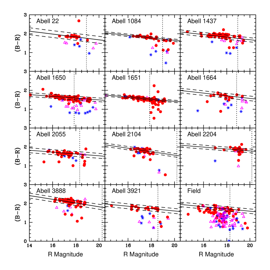
Figure 6: Colour–magnitude diagrams for the 11 clusters used in this work. Cluster members within 2 Mpc of the cluster centre are plotted. The biweight fit to these distributions is shown as the solid line; the parallel flanking dashed lines show the $1\sigma$ uncertainty in the colour. The vertical dotted lines denote $M_{V}=-20$ which is used to define the sample for the biweight fit. The lower right corner displays our field sample for comparison. This is constructed from non-cluster members and evolved to $z\sim 0.1$; the CMR lines are to illustrate where the CMR would be (we note that others do report the existence of a CMR for field ellipticals; e.g. see Bell et al. 2004) at this redshift; see Figure 2 of P02. The galaxies are coded upon the spectroscopic types: solid (red) circles are k types; open (magenta) triangles are k+a and a+k types; starred (blue) points are e types.

The more luminous early-type galaxies (ellipticals and S0s) within local clusters are known to exhibit systematically redder integrated colours than the late-types (Visvanathan & Sandage 1977). These galaxies also demonstrate a tight correlation between their colours and magnitudes: the colour-magnitude relationship (CMR; e.g. Bower, Lucey and Ellis 1992). For sub-L^⋆ galaxies, Kodama & Arimoto (1997) demonstrate that the slope of the colour-magnitude relation (assuming that the stellar populations are formed in a single event) could be due to the mean stellar metallicity (as suggested by Dressler 1984), with the scatter around the relation being due to age effects (Kodama et al. 1999). Fainter galaxies on the CMR may have been constructed from the fading or disk stripping of later-type galaxies, thus leaving a bulge with a small amount of younger stars present.

Following earlier studies by Abraham et al. (1996) and Terlevich et al. (2001), P02 and Wake et al. (2005) suggest that the CMR of clusters evolves bluewards with increasing clustocentric radius and decreasing local galaxy density. Their investigations, however, are made in the absence of spectroscopy by making a statistical correction to remove the contaminating field population. By employing spectroscopic membership, colour-magnitude diagrams are now constructed for spectroscopically-confirmed cluster members.

We use a biweight method to fit the CMR in an identical manner to that used by P02 (see also Beers, Flynn & Gebhardt 1990; Press et al. 1992). The spectroscopically-coded colour-magnitude diagrams for our eleven clusters whose galaxies are within a projected radius of $r_{p}<2$ Mpc of the cluster core are presented in Figure 6 with the biweighted fits to their CMRs.

Figure 7: Colour histograms of the composite cluster split on local galaxy density, $\Sigma$. The best fitting Gaussians for each bin are displayed as the dotted curves. The peak of the richest bin is noted on each panel by the vertical solid line whilst the peak of each individual bin is shown as the dashed vertical line. A blueward shift in the peak of the CMR is seen with decreasing local galaxy density at a rate of $d(B-R)/dlog(\Sigma)=-0.062\pm 0.009$.

To proceed, we now exploit the homogeneity of our clusters and combine them to make a composite. This is performed in the same manner as P02. Briefly, we have to transform the colours, magnitudes and positions of the galaxies onto a common scale. The apparent magnitudes are evolved to a median redshift of $z=0.12$ using the relative magnitudes of $L^{*}$ galaxies. The colours are dealt with by reducing the observed CMRs to provide colour information relative to the fitted relation and then transformed to $z=0.12$. Positions are moved onto a common scale by scaling to a fixed metric size. The relative merits of these transformations are discussed in detail by P02 and Wake (2003). Here it is sufficient to note that our clusters are a homogeneously selected sample with similar X-ray luminosities (i.e. cluster masses), therefore normalizing to a fixed metric size or to $r_{200}$ (Table 2) makes no significant differences to the results presented (cf. Wake et al. 2005 whose sample spans a factor of over 100 in X-ray luminosity). Finally, we create colour histograms of the composite cluster down to a limiting magnitude of $M_{V}=-20$ to search for any variation. Since our composite spectroscopic sample is much smaller than the full photometric one used in P02, we restrict our radial bins to be 2 Mpc annuli. To better identify these histogram’s peak values and quantify the radial blueing, we fit them with Gaussians using a $\chi^{2}$ minimization method. More extensive details of our fitting routine can be found in P02. These Gaussians are tabulated in Table 3. The peak colour of the CMR in the composite cluster evolves blueward at a rate of $d(B-R)/dr_{p}=-0.011\pm 0.003$ which is a rate some $2.2\sigma$ smaller than found from the photometric method of P02: $d(B-R)/dr_{p}=-0.022\pm 0.004$. Therefore those galaxies in the cluster outskirts may have luminosity-weighted mean stellar populations up to 3 Gyr younger than those in the cluster centre assuming $d(B-R)/dt=0.03$ mag per Gyr (Kodama & Arimoto 1997; see also Moran et al. 2005). One can also interpret Table 3 as showing that most of the radial blueing occurs within the central $\sim 3$–$4$ Mpc of the cluster centre. This would make the rate much steeper and inline with the radial colour changes noted by Gerken et al. (2005). It is also possible that at these large radii from the cluster centre, we may have a mixed galaxy population of those that have already been through the cluster centre and those that are infalling for the first time (e.g. Rines et al. 2005); we will explore this scenario in Section 5 in greater detail.

To examine this trend in a somewhat more general way we use local galaxy density, $\Sigma$, instead of clustocentric radius. The local galaxy density is estimated from the photometric catalogue by finding the surface area on the sky that is occupied by a given galaxy and its 10 nearest neighbours down to $M_{V}=-20$. As with the photometric method, this value will be overestimated due to background galaxy contamination, therefore we correct these values by subtracting off a constant density computed from the median local density of a field sample (P02). Since the range in $\Sigma$ is large, we work in logarithmic values and generate six bins covering three orders of magnitude in $log(\Sigma)$.

For each of these bins, we create a colour histogram from the composite spectroscopic cluster sample and fit Gaussians to them using our $\chi^{2}$ minimization method. The result of this analysis is presented in Figure 7 and tabulated in Table 3. Here, the peak colour of the CMR evolves bluewards with local galaxy density at a rate of $d(B-R)/dlog(\Sigma)=-0.062\pm 0.009$ which is, again, accompanied by a broadening of the CMR peak. Like the radial blueward trend, the trend with local galaxy density is smaller than the one found by the photometric method in P02 by $\sim 1\sigma$: $d(B-R)/dlog(\Sigma)=-0.076\pm 0.009$.

Table 3: Peak colour and full width of the variation of the composite CMR with both clustocentric radius and local galaxy density as derived from fitting Gaussians to the colour distributions (see also Figure 7).

Sample	Peak $(B-R)_{M_{V}=-21.8}$	$\sigma_{Peak}$
Radius (Mpc)
0–2	1.86 $\pm$ 0.01	0.12 $\pm$ 0.02
2–4	1.78 $\pm$ 0.03	0.14 $\pm$ 0.03
4–6	1.77 $\pm$ 0.04	0.16 $\pm$ 0.05
6–8	1.77 $\pm$ 0.07	0.21 $\pm$ 0.06
log10 (Local Galaxy Density)
$>$ 2.0	1.87 $\pm$ 0.01	0.12 $\pm$ 0.02
1.5–2.0	1.83 $\pm$ 0.02	0.14 $\pm$ 0.03
1.0–1.5	1.84 $\pm$ 0.04	0.15 $\pm$ 0.05
0.5–1.0	1.80 $\pm$ 0.05	0.15 $\pm$ 0.06
$-$0.5–0.5	1.78 $\pm$ 0.07	0.16 $\pm$ 0.06
$<-$0.5	1.77 $\pm$ 0.09	0.18 $\pm$ 0.08

From Figure 7 and Table 3, we are also able to examine how the width of the CMR changes with environment. The Gaussians fitted to these data are used to compute $\sigma_{\rm Peak}$, the CMR’s width. The width increases by some $\sim 0.1$ across the range studied, consistent with our previous findings (P02). We note, however, that even though we are using Gaussians to parametrize the CMR’s, there is no physical reason why the CMR should be well fit by a such a curve.

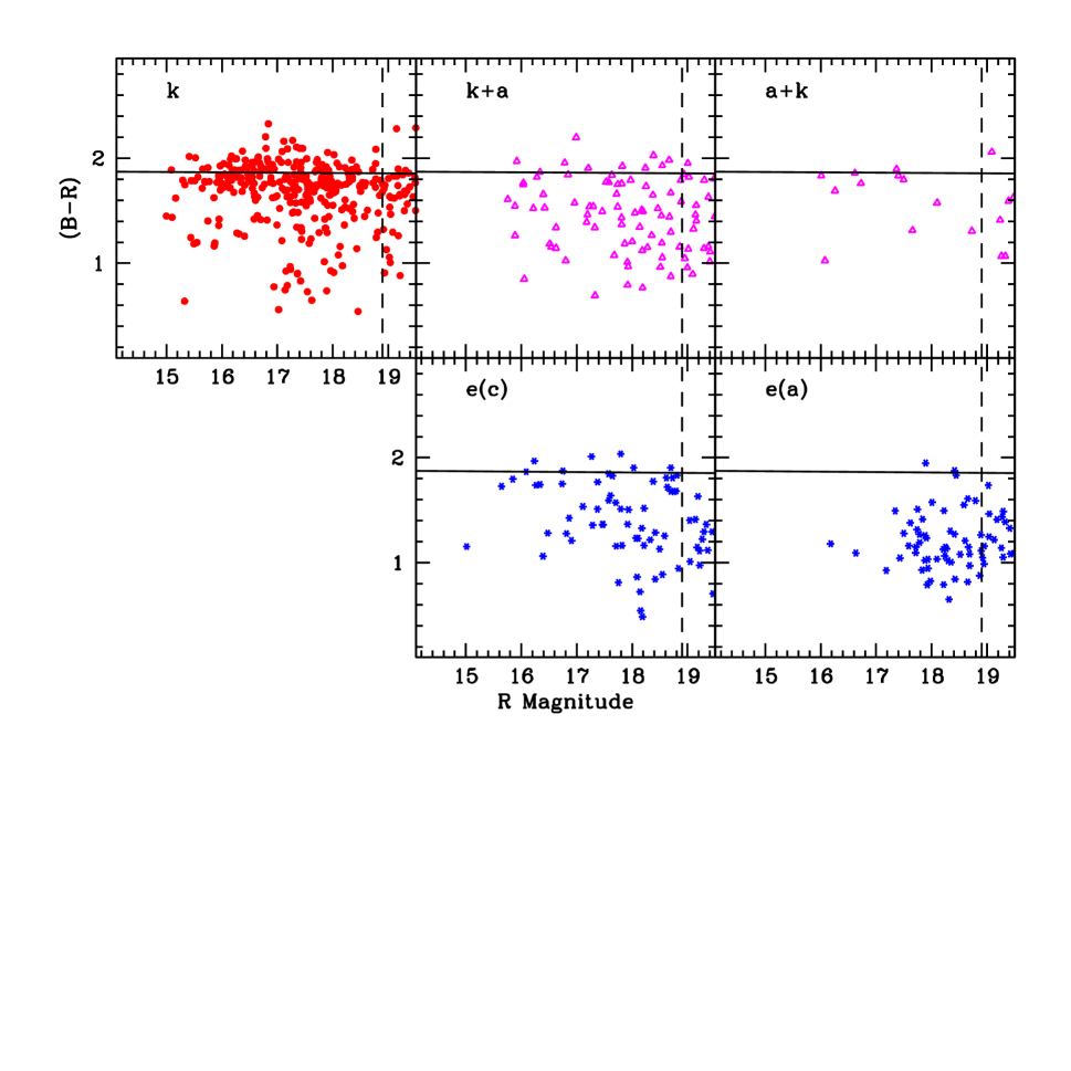
Figure 8: Colour-magnitude diagram for the composite cluster coded upon spectral type. The vertical dashed line denotes the fiducial magnitude cut $M_{V}=-20$ that we use. The horizontal solid line is the position of the composite cluster’s best fit CMR (note that the slope of the CMR has been removed in producing the composite cluster).

To better parametrize the changes in the shape of the CMR distribution we look at the trends in the quartile points with radius. The reddest galaxies on the CMR, evaluated by computing the 30^th percentile of the colour distribution, possess a near constant $(B-R)$ colour over the range of projected radius and local galaxy density probed in this study. Conversely, the bluer members, examined using the 70^th percentile, exhibit a strong blueward shift. This result is very similar to the P02 result (see Figure 7 of P02; also see Figure 13 of Wake et al. 2005).

One caveat in this analysis is that the best sampled systems such as Abell 3888 possess a greater weight in the composite cluster than the poorest sampled (e.g. Abell 1664). To explore this issue in more depth, we normalize all the clusters to have the same sampling and re-construct our composite cluster. Repeating the above experiments results in a change of rate in $d(B-R)/dr_{p}$ and $d(B-R)/dlog(\Sigma)$ by no more than $1.5\sigma$ – i.e. no significant change. Therefore, whilst there are cluster-to-cluster variations in this sample, we emphasize that the LARCS sample is an homogeneously X-ray selected one, and such variations are therefore minimized.

5.2 Populations on the CM plane

With the peak colour of the CMR progressing blueward with radius and local galaxy density, we may expect that the mean colour of the passive k-type galaxies on the CMR will also reflect these changes.

Figure 8 shows the colour magnitude diagrams of the different spectroscopic types in the composite cluster. Histograms of the colour distribution are shown in Figure 9 down to $M_{V}=-20$. These colour distributions show an number of interesting features. In the k-type class, there are a number of apparently non-starforming galaxies with colours bluer than the CMR and a small number of redder ones. The bulk of the k-types, however, do possess colours consistent with the CMR; $\sim$ 85 per cent of the population lies in the range $1.6<(B-R)<2.0$. Although there appears a large scatter in the k-type galaxies, it is no more than the scatter from the individual clusters (Figure 6). The poststarburst types (k+a and a+k) have a much flatter $(B-R)$ distribution. Whilst most lie blueward of the CMR, approximately 40 per cent of them have colours consistent with the CMR. We note, however, that some of the poststarburst types with colours consistent with the CMR are close to the boundary with k types (i.e. EW(H$\delta$)$\approx 3{\rm\AA}$) and may therefore have been misclassified (see above). Also, the k+a colour distribution appears to have a much larger scatter than the a+k one. However, with the small number (20) of a+k galaxies available to us (Figure 6), any firm conclusion about colour differences between the a+k and k+a populations is likely premature. The emission line types (e(a) and e(c)) are qualitatively different distributions, exhibiting significant fractions of blue ($(B-R)<1.6$) galaxies (55 and 90 per cent respectively). Indeed, the e(a) class is by far the bluest and faintest class of galaxy reflecting its characteristic vigorous on-going star-formation, whilst the e(c) types have a colour distribution similar to the k+a types.

On the issue of galaxy colours, we noted that Figure 8 shows a small yet significant population of blue passive (k type) galaxies ($B-R<$ 1.6) and very red galaxies ($B-R>$ 2.0; i.e. redder than the CMR ridge). To investigate the stellar populations of these galaxies, we combine together multiple spectra using the IRAF task scombine to improve the signal to noise ratio instead of using individual EW measurements from each galaxy (Figure 10). In the combined spectra, each individual spectra is weighted according to our completeness function in order to remove luminosity differences.

We find that the shape of the combined blue k-type spectra (bottom of Figure 10) is much more like a typical spiral galaxy than for the CMR sample. But compared to those galaxies on the CMR, the blue k-type galaxies have a small amount of [Oii]$\lambda 3727\rm{\AA}$ present coupled with obvious H$\beta$ and [Oiii]$\lambda 5007\rm{\AA}$ emission lines. The EW of this [Oii]$\lambda 3727\rm{\AA}$ is 2.6Å and hence on average these galaxies have 1.5 to 2 $\sigma$ [Oii]$\lambda 3727\rm{\AA}$ emission individually which in the MORPHs spectroscopic classification system ensures that they are typed as k’s. Meanwhile, the EW of the H$\beta$ and [Oiii]$\lambda 5007\rm{\AA}$ lines are 2.6 and 2.8 $\rm{\AA}$ respectively. We suggest that these passive blue galaxies have suffered some recent star formation which has perturbed their luminosity-weighted broadband colours. If their modest star formation rate ceases, then they are likely to quickly evolve on to the CMR (see Figures 6 and 7 of Kodama & Bower 2001).

The very red galaxies (top spectra of Figure 10) are similar to those on the CMR; lacking obvious [Oii]$\lambda 3727\rm{\AA}$ emission combined with small amounts of H$\delta$. Therefore, we tentatively suggest that these very red cluster galaxies have colours that are rather dust affected or are super-metal-rich. If they are dust affected, then it would not only affect their colours, but also produce an absence of UV emission lines.

Figure 9: Colour distribution of the different spectroscopic types contained within the composite cluster from Figure 8 with a magnitude cut-off of $M_{V}=-20$.

Figure 10: Restframe combined k type spectra (non-fluxed) for galaxies in the composite cluster with $(B-R)<1.6$ (bottom), $1.6<(B-R)<2.0$ (centre) and $(B-R)>2.0$ (top). Key spectral features are marked (top and dotted lines).

Although we have no detailed morphological classifications for our sample (Pimbblet 2001), we can use the distribution of our galaxies on a plane of concentration index (CI) and maximum surface brightness ($\mu_{\rm MAX}$) to look for changes in the morphological mix within the composite cluster (P01; Abraham et al. 1994). On the CI–$\mu_{\rm MAX}$ plane, early-type galaxies populate the high-concentration and high surface brightness region, with later-types typically having lower concentrations and fainter maximum surface brightnesses (P01). Comparing the distribution in CI–$\mu_{\rm MAX}$ of galaxies, we find that the very red sample is statistically the same as those galaxies drawn from the CMR. However, the blue k-type sample is composed of many more low $\mu_{\rm MAX}$ plus low CI galaxies than the CMR sample is. Applying a two dimensional Kolmogorov-Smirnov (K-S) test (Fasano & Franceschini 1987) to the CI–$\mu_{\rm MAX}$ distribution we find that the blue k-types are unlikely to have been drawn from the same parent population as the CMR sample at a 98 per cent confidence level. Since late-type galaxies in the field typically have much stronger [Oii]$\lambda 3727\rm{\AA}$ (Jansen et al. 2000) for their observed continuum colours, the blue k types are not normal disc systems. We suggest that these galaxies may therefore be anaemic late-types (i.e. similar to late-type galaxies except they possess low or insignificant amounts of emission) analogous to those observed at higher redshifts by Poggianti et al. (1999) and Balogh et al. (2002). At most, they comprise $\sim$ 2 per cent of the whole cluster population at $z\sim 0.1$ which is somewhat lower ($2\sigma$ significance) than the $6.5$ per cent reported by Balogh et al. (2002) across 10 $z\sim 0.25$ clusters for their anaemic late-type population.

Table 4: Spectroscopic classifications of cluster galaxies using the MORPHs system. Note that we find no e(a,b) types in our clusters while only A1664 and A2055 have any e(b) type galaxies. The numbers are all percentages and completeness function weighted (Figure 3). The final rows are for our composite cluster and field sample: constructed from the individual cluster observations and weighted by the completeness function. The column headed ‘Cluster Morphology’ gives a coarse indication of the general state of the cluster from work presented in P02 and from visually inspecting archival ROSAT X-ray imaging of our clusters.

Cluster	n(gal)	Percentage						Cluster
		k	k+a	a+k	e(c)	e(a)	e(b)	Morphology
Abell 22	67	54 $\pm$ 5	15 $\pm$ 3	0 $\pm$ 1	18 $\pm$ 3	12 $\pm$ 2	nil	Regular to intermediate cluster
Abell 1084	122	59 $\pm$ 4	19 $\pm$ 2	1 $\pm$ 1	12 $\pm$ 2	9 $\pm$ 2	nil	Irregular cluster
Abell 1437	224	67 $\pm$ 3	8 $\pm$ 1	4 $\pm$ 1	11 $\pm$ 1	10 $\pm$ 1	nil	Regular cluster
Abell 1650	208	67 $\pm$ 5	9 $\pm$ 3	0 $\pm$ 1	14 $\pm$ 3	10 $\pm$ 2	nil	Regular cluster
Abell 1651	208	75 $\pm$ 7	14 $\pm$ 2	3 $\pm$ 1	6 $\pm$ 1	2 $\pm$ 1	nil	Regular cluster
Abell 1664	123	51 $\pm$ 4	10 $\pm$ 2	2 $\pm$ 1	20 $\pm$ 2	15 $\pm$ 2	1 $\pm$ 1	Highly irregular cluster
Abell 2055	107	77 $\pm$ 7	15 $\pm$ 3	0 $\pm$ 1	7 $\pm$ 2	1 $\pm$ 1	0 $\pm$ 0	Regular cluster
Abell 2104	156	47 $\pm$ 4	25 $\pm$ 3	7 $\pm$ 2	15 $\pm$ 2	4 $\pm$ 2	nil	Intermediate cluster
Abell 2204	125	66 $\pm$ 7	11 $\pm$ 3	5 $\pm$ 3	16 $\pm$ 4	1 $\pm$ 1	nil	Intermediate cluster
Abell 3888	201	70 $\pm$ 5	12 $\pm$ 2	3 $\pm$ 2	10 $\pm$ 2	7 $\pm$ 2	nil	Intermediate cluster (see Girardi et al. 1997)
Abell 3921	126	56 $\pm$ 5	20 $\pm$ 4	1 $\pm$ 1	14 $\pm$ 3	6 $\pm$ 2	nil	Undergoing merger event (Ferrari et al. 2005)
Composite	1667	63 $\pm$ 2	14 $\pm$ 1	2 $\pm$ 0	13 $\pm$ 1	7 $\pm$ 1	0 $\pm$ 0	N/A
Cluster $<r_{200}$	692	71 $\pm$ 3	10 $\pm$ 1	1 $\pm$ 0	10 $\pm$ 1	3 $\pm$ 1	nil	N/A
Cluster $>r_{200}$	975	59 $\pm$ 3	16 $\pm$ 1	1 $\pm$ 0	16 $\pm$ 1	9 $\pm$ 1	0 $\pm$ 0	N/A
Field	853	48 $\pm$ 3	20 $\pm$ 1	3 $\pm$ 1	18 $\pm$ 2	6 $\pm$ 1	0 $\pm$ 0	N/A

5.3 Spectral populations in individual clusters

We present the breakdown by spectral class of the cluster members and a field sample in Table 4. The majority of the clusters have a dominant k component, typically accounting for half to three-quarters of the entire cluster population to $L^{\star}+2$. There are a significant number of post-starburst galaxies (k+a and a+k), accounting for a further $\sim$10 to 20 per cent. This is in contrast with the recent study of the similarly X-ray luminous local Coma cluster by Poggianti et al. (2004) who find no post-starburst galaxies at such bright magnitudes. Moreover, unlike Poggianti et al. (2004), our post-starburst galaxies are not preferentially situated anywhere in particular in the cluster, regardless of their colour. The actively starforming fraction tends to be marginally greater than the poststarburst fraction, amounting to $\sim$15 to 25 per cent of most of our clusters.

In contrast to the MORPHs clusters (Table 4 of Poggianti et al. 1999), our cluster core regions are much less active than their $z\sim 0.4$ cousins; i.e. higher passsive fractions and lower emission fractions in general. To better compare directly to the MORPHs clusters, we note that the Poggianti et al. (1999) sample is limited to $M_{V}=-19$; roughly equal to $M^{*}+1.5$ (Dressler et al. 1997) and that their spatial extent is roughly 2 Mpc at their median redshift – about or just below $r_{200}$ for our clusters. By imposing the same limits on our composite cluster sample, the fractions presented for the $r_{p}<r_{200}$ sample in Table 4 do not change by more than $2\sigma$ in a given spectral type. We tentatively suggest therefore, that the e(b) class has vanished to all intents and purposes at $z\sim 0.1$ whereas Poggianti et al. (1999) find about 5 per cent of cluster members are e(b) types at $z\sim 0.4$. This is only tentative as 5 per cent differences between our sample and Poggianti et al. (1999) are of marginal significance – about 2.5$\sigma$. Further, from $z\sim 0.4$ to $z\sim 0.1$, the e(c) fraction remains approximately the same; the e(a) fraction falls by about 4 per cent (not significant); the combined k+a & a+k faction falls by 5 per cent (not significant); while the k fraction increases by some 15 per cent ($>3\sigma$ significance). The k types may be the endpoints of active galaxies once their activity fades and hence it is not surprising that evolution is most marked in this subsample compared to the different flavours of active galaxies. We also note that MORPHs is a mixed cluster sample spanning a range in richness and are not all X-ray luminous.

Although our sample has uniform X-ray selection, there also appears to be real variation between our clusters. For example, our most irregular cluster, A1664, is marked out by a very small ratio of active to passive types (e(a)+e(c) : k $=1:1.5$) whereas A2055 and A1651 both have a much larger ratio ($\approx 1:9.5$). Such differences in passive : active ratios can not be wholly accounted for by differences in global cluster parameters such as X-ray luminosity or velocity dispersion (Table 2). However, the coarse morphologies of the clusters (see Table 4; our coarse morphologies are derived from visually inspecting ROSAT X-ray maps and two dimensional galaxy distribution from P02) show that the more irregular systems (e.g. A1664 and A3921) tend to display a higher incidence of active galaxies than their more regular counterparts (e.g. A1437). We note that A1664 is likely in the early phases of merging and the enhanced active fraction could be a result of this. While, A3921 is in the middle phase of merging (Ferrari et al. 2005) and is less active, but displays many more post-starburst types. Moreover, the clusters with the smallest fractions of k type galaxies also appear to be the ones with the most non-Gaussian appearing velocity distributions (Figure 4). To test this, we fit Gaussians to the $N(z)$ distributions shown in the inset panels of Figure 4, allowing the normalization, mean velocity and $\sigma$ of the fits to all be free parameters, and find the $\chi^{2}$ of each fit. In Figure 11 we show the relationship between the $\chi^{2}$ and the fraction of active galaxies in each cluster. We find a correlation between these variables, at a $3\sigma$ level. Therefore, the clusters that possess the least Gaussian velocity dispersions tend to be the ones that either are actively starforming or have recently formed stars.

Figure 11: Fraction of active galaxies (i.e. 1 - fraction of k types) in the clusters (Table 4) versus the $\chi^{2}$ of a Gaussian fit to their velocity distributions Figure 4. The solid line is a fit to the points and is $3\sigma$ away from a slope of zero. Due to this mild correlation between the two variables, we suggest that the clusters with the least Gaussian velocity distributions also have the lowest fraction of k type galaxies, or equally, are the most active clusters.

We conclude that even in an homogeneously X-ray selected sample of galaxy clusters, individual clusters can show real and significant variation from cluster to cluster, probably reflecting their recent infall histories. The only correlation with fractions of different spectral types is the mild anti-correlation between Gaussian velocity distributions and k type fraction. We suggest that these variations between the clusters are likely driven by local processes as there is no clear correlation with other global parameters such as $L_{X}$ or $\sigma_{z}$ with the highest / lowest fractions of post-starburst or active galaxies.

5.4 Environmental Dependence of Line Strengths

The trends in the characteristic colour of the CMR we see as a function of radius or local galaxy density should be mirrored by changes in the spectroscopic properties of these galaxies. In particular, if the variation in the $(B-R)$ colour comes about from its sensitivity to the age of the stellar population (e.g. Searle et al. 1973), then we would expect to see increasing signs of youth in the spectra of galaxies on the CMR in the lower density outskirts of the clusters. The Balmer absorption line, H$\delta$, provides a useful indicator of mean stellar age in non-star forming systems (although we note that H$\delta$ does not trace only age; Thomas et al. 2004). Indeed, Terlevich et al. (1999) demonstrate the relationship between deviations in the $(U-V)$ colour of galaxies away from the CMR and the equivalent deviations in the strength of Balmer absorption lines from observations of early-type galaxies in the Coma cluster. Based on a CMR zeropoint shift of $\Delta(B-R)\sim 0.07$ for typical galaxies out to 4 Mpc (Table 3), we estimate (using data from Terlevich et al. 1999; see also P02) that this population should show an enhanced Balmer absorption of $\sim$ 2.8Å equivalent width.

Using only the non-starforming population of galaxies (i.e. the emission line types of galaxies with EW[Oii]$\lambda 3727\rm{\AA}>5.0$ are excluded) that lie on the CMR, a detection of an increase in the mean strength of the H$\delta$ absorption line by $\sim 2.2{\rm\AA}$ from the cluster core region to the outskirts of the cluster is confirmed at $>3.5\sigma$ (Table 5). However, this level of change in H$\delta$ could have been expected by 4 Mpc rather than in the outskirts (i.e. by 8 Mpc). We note that most of the colour change occurs within the central $\sim 4$ Mpc and further colour changes with radius are minimal. Therefore whilst the prediction remains valid at 8 Mpc; at 4 Mpc, we are at least 2.5$\sigma$ away from the prediction of Terlevich et al. (1999). This may be related to the fact that Terlevich et al. (1999) study the Coma cluster which is at much lower redshift than our sample. Fitting a line to the points presented in Table 5 weighted by their errors yields a rate of $d$H$\delta/dr_{p}=0.35\pm 0.06$. The trend with local galaxy density, however, is more noisy. The highest density bin (log($\Sigma$) $>2.0$) has a large error due to the comparatively small number of galaxies present. Weighting by the errors in Table 5 also gives a rate of $d$H$\delta/dlog(\Sigma)=0.66\pm 0.15$ with decreasing density. To ascertain whether radius or local galaxy density is more important, we compute the relationship between the two variables. Then, for given radii (or local galaxy densities), we find the corresponding density (or radius) and compare which of the two rates shows the stronger trend. In most cases, local galaxy density appears to be more important (stronger) than radius from the cluster centre, although the differences at large radii ($>3$ Mpc) become increasingly less significant. Therefore, we tentatively suggest that local galaxy density is a more fundamental parameter than radius (in contrast, see Whitmore et al. 1993). We also note that we have included the more irregular clusters in this analysis (Table 4); our result does not change (i.e. local galaxy density being more important) even if we exclude these clusters from the composite.

Table 5: Increase of the mean strength of the H$\delta$ absorption line in passive galaxies with colours consistent with the CMR (within $\pm 1\sigma$) as a function of both cluster radius and local galaxy density in the composite cluster.

Sample	Mean EW(H$\delta$) (${\rm\AA}$)
Radius (Mpc)
0–2	0.39 $\pm$ 0.16
2–4	1.06 $\pm$ 0.28
4–6	1.24 $\pm$ 0.36
6–8	2.56 $\pm$ 0.69
log (Local Galaxy Density)
$>$ 2.0	0.83 $\pm$ 0.40
1.5–2.0	0.36 $\pm$ 0.25
1.0–1.5	1.05 $\pm$ 0.32
0.5–1.0	0.51 $\pm$ 0.41
$-$0.5–0.5	1.07 $\pm$ 0.40
$<-$0.5	1.95 $\pm$ 0.46

Gómez et al. (2003) and Lewis et al. (2002; see also Balogh et al. 2004) report that the starformation rate increases significantly at at large distances from the cluster core (and similarly, for small values of local galaxy density). For EW[Oii]$\lambda 3727\rm{\AA}$, Gómez et al. (2003) demonstrate that the median value starts to differ significantly from the field value at about 3–4 virial radii ($r_{V}$) from the cluster core. This critical radius corresponds to roughly $r_{p}\approx 4$ Mpc (or $\sim$ few galaxies per Mpc²) for our survey and assumed cosmology.

In Figure 12, we plot the median EW [Oii]$\lambda 3727\rm{\AA}$ for all our cluster galaxies brighter than $M^{*}+1$ (to match Gómez et al. 2003) as a function of $r_{p}$ and $\Sigma$. For comparison, we have also constructed a $z\sim 0.1$ ‘field’ sample. This is done by taking all galaxies in the range $0.07<z<0.16$ (to match the redshift of the LARCS clusters) and then excluding all cluster members and other significant structure (e.g. the wall in Abell 22; Pimbblet, Edge & Couch 2005; Abell 1079 which is in the periphery of Abell 1084; Pimbblet & Drinkwater 2004; P02). From this sample, we compute the 75th and 25th quartiles of the EW [Oii]$\lambda 3727\rm{\AA}$ distribution to compare directly with the cluster sample; see Figure 12. The median EW [Oii]$\lambda 3727\rm{\AA}$ increases from the cluster core to the outskirts of the composite cluster, with a ‘break’ at around 3–4 Mpc. The changes in the median shown in Figure 12 are due to a decline of the upper quartile. The break at 3–4 Mpc corresponds well with the characteristic radius found by Gómez et al. (2003). In order to test where the cluster population becomes significantly different from the field sample, we employ a KS test on the two distributions. We find that the cluster EW [Oii]$\lambda 3727\rm{\AA}$ distribution starts to differ significantly ($>1\sigma$; 68 per cent level) from the field distribution at below $r_{p}<3.8$ Mpc (Figure 12). Such a radius is very comparable to the Gómez et al. (2003) result ($r_{p}\approx 4$ Mpc; vertical dotted line in Figure 12). In terms of local galaxy density, this radius corresponds to $\approx 1.3\pm 0.2$ galaxies per square Mpc (c.f. $\sim 1$ galaxy per square Mpc found by Gómez et al. 2003).

5.5 Luminosity functions and phase-space diagrams

Figure 12: Median EW [Oii]$\lambda 3727\rm{\AA}$ as a function of projected radius from the cluster centre (left) and local galaxy density (right). The error bars are 1$\sigma$ on the median values. Each bin contains 100 cluster galaxies. The upper and lower curves are the 75th and 25th quartiles of the cluster EW distribution. The horizontal solid lines are the 75th and 25th quartiles of the field sample. The dotted vertical line denotes the critical radius (density) obtained by Gómez et al. (2003). There is a break in cluster EW [Oii]$\lambda 3727\rm{\AA}$ at about 3–4 Mpc ($\sim$ few galaxies per Mpc²) which corresponds well with the Gómez et al. (2003) and Lewis et al. (2002) results.

Figure 13: Luminosity distributions of the different spectral types in the combined cluster (solid line) and the field sample (dotted line). The cluster k types are much brighter than the others; indeed the relatively flat k+a/a+k distribution may be due to mixing bright k-types with real, fainter k+a/a+k’s. Meanwhile, the field sample appears to have a deficit of bright k+a/a+k galaxies in comparison to the cluster luminosity distributions.

Figure 14: Velocity–radius distributions of the different spectral types in the combined cluster. For reference, we superimpose the mass model from Figure 5 and a line at $\Delta{\rm v}/\sigma_{z}=0$. The more active types possess a larger velocity dispersion and are more likely to reside in the outer regions of the clusters.

To better understand the relationship between the different spectral classes in clusters and their evolution from higher redshift counterparts (i.e. Dressler et al. 1999; Poggianti et al. 1999), we now examine their absolute luminosity distributions (Figure 13) and orbital characteristics (Figure 14). The absolute magnitude distributions for k, k+a and a+k types are brighter than for the e(c) and particularly for the e(a) types (similar to the $z\sim 0.4$ sample from Dressler et al. 1999). However, Dressler et al. (1999) report that at $z\sim 0.4$, the distributions of k, k+a and a+k are indistinguishable, but in our sample at $z\sim 0.1$, the k+a and a+k luminosity function is much flatter than for the k types (Figure 13). This may be due to mixing bright k types with fainter, real k+a and a+k types as a result of scattering across the spectral type boundaries (Section 4.5).

Table 6: Dispersion in $\Delta$v / $\sigma_{z}$, relative to the k types, and average distance from the cluster centre per spectral type from Figures 14 and 15. The star-forming types tend to reside at the outskirts of the cluster and possess a much larger velocity dispersion.

Type	$\sigma$ ($\Delta$v / $\sigma_{z}$)	radius / $r_{200}$
k	1.00	$1.01\pm 0.06$
k+a	1.61	$1.49\pm 0.17$
a+k	3.41	$1.73\pm 0.23$
e(c)	3.20	$1.76\pm 0.21$
e(a)	5.85	$2.09\pm 0.16$

To examine how the different spectroscopic types are distributed within the composite cluster, we construct both velocity–radius plots of the different spectral types (Figure 14) and a cumulative radial distribution, derived for all galaxies brighter than $M_{V}=-20$ (Figure 15). The passive k-type galaxies dominate the core regions of the cluster ($r_{p}<r{200}$) whilst the other types occur more frequently beyond $r_{200}$ and are generally of higher velocity dispersion. To quantify this, we compute a normalized velocity dispersion, $\sigma$($\Delta$v / $\sigma_{z}$), and mean radius of each of the different spectral types (Table 6). This demonstrates that the active types are much more likely to reside in the outskirts of the cluster (similar to the finding of Gerken et al. 2005 that the fraction of emission line galaxies increases strongly beyond 2 Virial radii) and possess a much higher velocity dispersion range than the poststarburst or the passive types. This is confirmed in Figure 15, where the passive k-type galaxies are distinctly seen to be the most centrally concentrated whilst the emission line galaxies preferentially avoid the cluster centre, possessing a more extended distribution. The k+a types, meanwhile, are half-way between the k and e(c) types.

Finally, in Figure 13, we also plot the luminosity distribution of field galaxies at $z\sim 0.1$ to compare with our composite cluster sample. Our field sample contains an obvious lack of bright k+a/a+k galaxies in comparison to the cluster sample. We display the combined bright k+a/a+k cluster galaxy spectra in Figure 2. Whilst these combined spectra do possess enhanced H$\epsilon$ and H$\gamma$, there is a concern over whether the bright k+a/a+k population seen in the clusters are ‘real’ E+A galaxies. For example, Blake et al. (2004) find that of their 243 H$\delta$ strong E+A galaxies, 60 per cent have indications of ongoing star formation (H$\alpha$ emission; H$\gamma$ and H$\beta$ are presumably subject to emission-filling and [OII] is dust-obscured). Our cluster members do not have sufficient spectral coverage to reach H$\alpha$, so this cannot be checked. But in the absence of significant [OII], it could be that like their E+A sample, ours may also be dust affected (e.g. dusty disks).

We can assess what would happen to our sample if we had have used a non-MORPHS, stricter definition of E+A galaxies: EW’s of H$\delta$, H$\gamma$ and H$\beta$ all being greater than 4 ${\rm\AA}$. The result is a loss of over two thirds of our k+a/a+k sample and we end up with some rather strange ‘k’ types that have very strong H$\delta$ EW! After all, there is much scatter in the H$\delta$ versus H$\gamma$ EW relationship (see Figure 1 of Blake et al. 2004). Moreover, if k+a galaxies are selected on this strict basis, it is very unlikely that they will have any H$\alpha$ emission (Blake et al. 2004).

To test the degree of misclassification in the sample, we now perturb the EW measurements of [OII] and H$\delta$. This is done by adding a random Gaussian sampling of the EW errors to the original measurements 100 times. With each new measurement, we compute what spectral class would have been assigned to the galaxy. In the combined cluster (Table 4) this re-typing would increase the number of k type galaxies at the expense of the k+a types. However, this increase is not very significant: no more than $1\sigma$. In the combined field fractions (Table 4), the perturbations result in an increase of the fractions of k and k+a types at the expense of a few e(c) and e(a) types. Again, however, this change is only by $\sim 1.5\sigma$.

Figure 15: Cumulative radial fraction per galaxy type in the combined cluster from Figure 14. The median radii for each type is noted in Table 6. The k-types are more centrally concentrated than the other types with poststarforming k+a types being half-way between k and e(c) types.

5.6 Backsplash

We have already noted that some of our results may be considered to be due to galaxy mixing from ‘backsplash’ galaxies. Backsplash galaxies are those that have already been inside the cluster virial radius ($\sim r_{200}$) but are now observed outside this radius (e.g. Gill, Knebe & Gibson 2005; Rines et al. 2005; Mamon et al. 2004; Balogh et al. 2000). Gill et al. (2005) show through their simulations that the backsplash population can be detected in a straight forward fashion as they will exhibit distinct kinematics: a more centrally peaked velocity distribution in the interval $1.4<r_{p}/r_{200}<2.8$. A non-zero velocity distribution peak would indicate that the galaxies in this interval are likely on their first infall. Rines et al. (2005) use this interval to show that backsplash cannot be wholly (or even primarily) the driving force behind galaxy transformations in clusters.

We are also able to test the backsplash scenario through our observations (Figure 14). A histogram of the galaxy velocities in the interval $1.4<r_{p}/r_{200}<2.8$ is presented in Figure 16. This velocity distribution is not peaked at zero or at a larger value – therefore our cluster population at these radii is neither a pure backsplash population (which would be expected to peak at zero velocity) or purely infalling for the first time (which would be expected to peak at about 0.3–0.5 $|\Delta v|/\sigma_{z}$ in Figure 16; approximately 400 kms^-1; Gill et al. 2005). This mixture of both backsplash and infalling galaxies is in line with the recent results of Rines et al. (2005). Further, our data show no significant difference in velocity distribution for emission line galaxies (e(a) and e(c)) versus non-emission line galaxies (k, k+a and a+k) using a standard K-S test. Therefore, we complement the result of Rines et al. (2005) that some emission line galaxies are likely to be backsplash ones and a pure backsplash model cannot account for the data. This is inline with the results of Gomez et al. (2003) and Lewis et al. (2002) that demonstrate that star formation is primarily a function galaxy density. Our earlier suggestion that local galaxy density is a more fundamental parameter than radius from a cluster centre is also reinforced because of this.

Figure 16: Distribution of cluster galaxies velocities in the interval $1.4<r_{p}/r_{200}<2.8$ as derived from Figure 14. Our galaxies are not significantly peaked around zero velocity, nor at a larger velocity, indicating that LARCS has a mixed population of backsplash galaxies and those that are infalling into the cluster for the first time.

6 Conclusions

In conclusion, this work presents, and analyzes, the spectroscopic observations of rich X-ray luminous galaxy clusters at $z\sim 0.1$. In total, we have amassed over 7500 moderate resolution spectra, giving an unprecedented view of galaxy clusters from their core out to beyond their virial radii. Of these spectra, about 1600 are galaxy cluster members across eleven $z\sim 0.1$ clusters with good signal to noise ratios. Easily two thirds of these cluster members are outside $r_{200}$, making our survey one of the widest-field, high completeness surveys of clusters at these redshifts to date.

• We confirm the result of P02 (see also Wake et al. 2005) of a radial colour gradient at fixed luminosity of $d(B-R)/dr_{p}=-0.011\pm 0.003$ from the cluster core out to at least 6 Mpc. The composite cluster also displays a colour gradient with local galaxy density of $d(B-R)/dlog(\Sigma)=-0.062\pm 0.009$ across three orders of magnitude in local galaxy density. In addition to these photometric gradients detailed here and in P02, we have also found spectroscopic gradients across our clusters, indicating the luminosity-weighted mean stellar population age in galaxies decreases with increasing radius ($d$H$\delta/dr_{p}=0.35\pm 0.06$), and decreasing local galaxy density ($d$H$\delta/dlog(\Sigma)=0.66\pm 0.15$). The effect is slightly stronger with local galaxy density than with radius.

• A break in the [Oii]$\lambda 3727\rm{\AA}$ EW versus radius relation occurs at roughly $r_{p}=4$ Mpc. This is equivalent to $\sim 1$–few galaxies per Mpc² and is consistent with the result found by others (Lewis et al. 2002; Gomez et al. 2003). Such a large radius is somewhat surprising for processes which rely on high gas or galaxy densities to influence the starformation of cluster galaxies. We therefore suggest that effects on the star formation histories of galaxies take place in the infalling substructures, which can have densities in the star formation break range of $\sim$few galaxies per Mpc², in a manner independent of the cluster environment. This break in radius is significantly different to the study made by Moran et al. (2005) who find a break at a radius of $\sim 1$ Mpc. This may be due to selection effects (Moran et al. 2005 sample galaxies down to $M^{\star}+1.6$, have a smaller radial extent and define ‘field’ values differently) or that they examine only a single cluster (the cluster is at $z=0.4$ and has an unusually large scatter in fundamental plane residuals in the cluster core region).

• Even though our clusters are selected above a fixed X-ray luminosity, the cluster themselves show significant differences between their galaxy populations (galaxies with old stellar populations; poststarburst galaxies and currently starforming galaxies). The ratio of actively starforming to passive types in our clusters spans a large range – $1:1.5$ through $1:9.5$. There appear to be no clear correlations between the fractions of different spectral types and global cluster properties such as $L_{X}$, $\sigma_{z}$ or (coarse) cluster morphology. However, we do find a mild anti-correlation between the Gaussianity of clusters velocity distributions and their fraction of k type galaxies. We suggest that the differences between the populations are probably the product of their recent accretion histories and are driven by local processes.

• There exist populations of galaxies both blueward and redward of the CMR that have similar spectral characteristics (i.e. old stellar populations with little or mild on-going starformation) to those galaxies lying on the CMR. We speculate that the redder population, which are morphologically indistinguishable from the CMR population, are dusty k types. The bluer population, meanwhile, are significantly less centrally concentrated and therefore we suggest that they may be the low redshift analogues to the passively evolving spirals found at higher redshifts (e.g. Balogh et al. 2002; Poggianti et al. 1999). These bluer galaxies may ultimately evolve on to the CMR.

• By constraining our $z\sim 0.1$ sample to the same radial extent and absolute magnitude range as the MORPHs sample, we find that the luminosity distributions and spectral populations of cluster galaxies have evolved since $z\sim 0.4$. In particular, our $z\sim 0.1$ sample has significantly ($>3\sigma$) more k type galaxies than their higher redshift counterparts. We suggest that the highly starforming e(b) class has declined (although the significance of this difference is only marginal at $\approx 2.5\sigma$). Certain other spectral types (k+a, a+k, e(a) and e(c)) show no significant changes.

• Our data do not highlight any single mechanism or scenario that can wholly account for the results presented here. For example, our population at $1.4<r_{p}/r_{200}<2.8$ consists of a mixture of both backsplash galaxies and galaxies that are infalling for the first time. Therefore star formation in these systems must be more fundamentally a function of local galaxy density rather than radius from the cluster centre. The break in EW measurements would not favour mechanisms that rely on high gas or galaxy density, so a mechanism such as strangulation cannot wholly account for our data. Mechanisms that only affect the high density cluster cores are not favoured either (e.g. ram pressure stripping or galaxy-galaxy harrassment).

This work follows Pimbblet et al. (2001; 2002) and is the third paper in a series based upon the LARCS survey.

Acknowledgments

We thank the referee, Bodo Ziegler, for his careful and constructive comments on this paper. We would also like to thank Michael Balogh, Julianne Dalcanton, Michael Drinkwater, Mary Hawkrigg, Tadayuki Kodama, Simon Morris, Ray Sharples and David Wake for productive comments and discussions on various aspects of this work.

KAP acknowledges support from an EPSA University of Queensland Research Fellowship, a UQRSF grant and PPARC. IRS and ACE acknowledge support from the Royal Society. WJC and EO’H acknowledge the financial support of the Australian Research Council. AIZ acknowledges support from NASA grant HF-01087.01-96. We thank the Observatories of the Carnegie Institution of Washington and the Anglo-Australian Observatory for their generous support of this survey. We especially wish to thank Terry Bridges and Geraint Lewis for their expert assistance at the telescope and advice during the spectroscopic data reduction stages.

Table 7: LARCS spectroscopic cluster catalogues. Entries of NA indicate that whilst the R band was observed, the B band was not (Pimbblet 2001; P01).

LARCS	RA	Dec.	R Mag	(B-R)	cz	$R_{TDR}$
Identifier	(J2000)	(J2000)			(km-1)
a22_01:1148	00 23 13.87	-25 45 34.0	17.40 $\pm$ 0.01	0.39 $\pm$ 0.01	-31 $\pm$ 16	15.4
a22_01:392	00 24 51.43	-25 50 57.2	18.38 $\pm$ 0.02	2.22 $\pm$ 0.07	101831 $\pm$ 72	2.6
a22_02:1155	00 21 32.76	-25 44 10.9	19.31 $\pm$ 0.05	2.24 $\pm$ 0.18	87177 $\pm$ 127	7.2
a22_02:1204	00 22 9.26	-25 45 19.8	18.44 $\pm$ 0.02	1.08 $\pm$ 0.03	28267 $\pm$ 51	5.6
a22_02:1225	00 21 59.53	-25 45 29.9	18.05 $\pm$ 0.02	0.85 $\pm$ 0.03	36457 $\pm$ 36	4.8
a22_02:1226	00 21 54.37	-25 45 29.9	19.83 $\pm$ 0.05	1.58 $\pm$ 0.08	94392 $\pm$ 17	0.1
a22_02:125	00 21 53.08	-25 33 3.3	17.22 $\pm$ 0.01	0.65 $\pm$ 0.01	67000 $\pm$ 37	2.6
a22_02:1258	00 21 46.66	-25 45 56.8	19.74 $\pm$ 0.05	1.62 $\pm$ 0.10	34119 $\pm$ 19	0.8
$\vdots$	$\vdots$	$\vdots$	$\vdots$	$\vdots$	$\vdots$	$\vdots$

Table 8: Other structures identified along the line of sight to the primary LARCS cluster targets. Entries of ‘NED02’ refer to objects that have multiple entries with the same name in the NED database – the 02 denotes that this is a secondary object not associated with the primary object of the same name.

Structure	$cz$ Range	$\overline{cz}$	$\sigma_{z}$	N(gal)	Comments
Identifier	(kms-1)	(kms-1)	(kms-1)
LARCS-22-Wall	30000–35000	33811$\pm$88	619${}^{+74}_{-54}$	$>$49	Part of candidate supercluster? (Pimbblet et al. 2005)
Abell 1079	38000–42000	39671$\pm$64	712${}^{+50}_{-42}$	46	Attempt to localize Abell 1079 in field of Abell 1084
LARCS-1437-A	24500–27500	25874$\pm$90	659${}^{+75}_{-56}$	40	Possibly Abell 1459(?)
LARCS-1650-A	33000–38000	35981$\pm$99	733${}^{+82}_{-62}$	54
LARCS-1651-A	40000–45000	41541$\pm$223	1370${}^{+193}_{-136}$	37	Possibly Abell 1658(?)
LARCS-1651-B	53000–57000	54972$\pm$116	811${}^{+97}_{-72}$	48	ZwCl 1300.9-0244(?)
LARCS-2055-A	8500–12000	10366$\pm$74	495${}^{+63}_{-45}$	44	Abell 2052
LARCS-2055-B	22000–26000	$22766\pm 152$	$861^{+135}_{-92}$	31
LARCS-2055-C	51000–57000	$53825\pm 174$	$955^{+155}_{-104}$	29
LARCS-2104-A	16000–20000	$17567\pm 184$	$902^{+170}_{-108}$	23	Abell 2103(?)
LARCS-2204-A	16000–18500	$17441\pm 50$	$360^{+42}_{-31}$	51
LARCS-2204-B	22000–25000	$23810\pm 41$	$393^{+32}_{-26}$	91
LARCS-2204-C	86000–88000	$87721\pm 36$	$235^{+31}_{-30}$	38
LARCS-3888-A	21000–24000	$22691\pm 118$	$781^{+100}_{-72}$	43	Possibly Abell 3896 NED02(?) (Batuski et al. 1999)
LARCS-3888-B	58000–65000	$61232\pm 224$	$1449^{+191}_{-137}$	41
LARCS-3921-A	37500–42200	$40208\pm 112$	$945^{+91}_{-71}$	70	Abell 3921 NED02 (Katgert et al. 1996)
LARCS-3921-B	47000–49000	$48114\pm 99$	$476^{+92}_{-58}$	22
LARCS-3921-C	60000–65000	$62893\pm 145$	$948^{+123}_{-88}$	42	AM 2250-633
LARCS-3921-D	85000–90000	$87505\pm 170$	$1050^{+147}_{-104}$	37

Appendix A: Spectroscopic catalogues

Table 7 gives the LARCS spectroscopic cluster catalogues for the observations used in this work. The full version of our spectoscopic catalogues will be made available in Synergy, the on-line version of the Monthy Notices of the Royal Astronomical Society. We note that a sub-set of these data have already been used by Pimbblet et al. (2005) and Krick, Bernstein & Pimbblet (2006).

Appendix B: Other structures

As can be seen from Figure 4, there are a number of other overdense structures (i.e. walls, clusters, etc.) along the line of sight to our primary LARCS cluster targets. Here, we attempt to characterize these structures by applying the ZHG technique to them. In doing so, we have only chosen those peaks in Figure 4 that are significant (N(gal)$>\sim$20 in a redshift range of $dcz=1000$ kms^-1) and relatively easy to isolate (i.e. no large spread in redshift space). As with the LARCS clusters, we make an initial guess of the velocity clipping to use by manual inspection of the velocity histograms (Figure 4). The results of this analysis are presented in Table 8. Note that since many of these structures are not wholly contained within the LARCS 2 degree field, we make no attempt to find the centroid of them. However, we do use individual members positions to aid in identifying likely corresponding clusters from the literature.

References

- [\citeauthoryearAbell1958] Abell G. O., 1958, ApJS, 3, 211
- [\citeauthoryearAbell, Corwin, & Olowin1989] Abell G. O., Corwin H. G., Olowin R. P., 1989, ApJS, 70, 1
- [\citeauthoryearAbraham et al.1994] Abraham R. G., Valdes F., Yee H. K. C., van den Bergh S., 1994, ApJ, 432, 75
- [\citeauthoryearAbraham et al.1996] Abraham R. G., et al., 1996, ApJ, 471, 694
- [Bailey, Taylor, Robertson, & Barden(2001)] Bailey J., Taylor K., Robertson G., Barden S., 2001, New Astronomy Review, 45, 41
- [\citeauthoryearBalogh et al.1997] Balogh M. L., Morris S. L., Yee H. K. C., Carlberg R. G., Ellingson E., 1997, ApJ, 488, L75
- [\citeauthoryearBalogh et al.1998] Balogh M. L., Schade D., Morris S. L., Yee H. K. C., Carlberg R. G., Ellingson E., 1998, ApJ, 504, L75
- [\citeauthoryearBalogh et al.1999] Balogh M. L., Morris S. L., Yee H. K. C., Carlberg R. G., Ellingson E., 1999, ApJ, 527, 54
- [\citeauthoryearBalogh, Navarro, & Morris2000] Balogh M. L., Navarro J. F., Morris S. L., 2000, ApJ, 540, 113
- [\citeauthoryearBalogh et al.2001] Balogh M. L., Christlein D., Zabludoff A. I., Zaritsky D., 2001, ApJ, 557, 117
- [\citeauthoryearBalogh et al.2002] Balogh M. L. et al., 2002, ApJ, 566, 123
- [\citeauthoryearBalogh et al.2004] Balogh M., et al., 2004, MNRAS, 348, 1355
- [\citeauthoryearBarnes & Hernquist1991] Barnes J. E., Hernquist L. E., 1991, ApJ, 370, L65
- [Batuski et al.(1999)] Batuski D. J., Miller C. J., Slinglend K. A., Balkowski C., Maurogordato S., Cayatte V., Felenbok P., Olowin R. 1999, ApJ, 520, 491
- [\citeauthoryearBeers, Flynn, & Gebhardt1990] Beers T. C., Flynn K., Gebhardt K., 1990, AJ, 100, 32
- [\citeauthoryearBekki, Couch, & Shioya2002] Bekki K., Couch W. J., Shioya Y., 2002, ApJ, 577, 651
- [\citeauthoryearBell et al.2004] Bell E. F., et al., 2004, ApJ, 600, L11
- [Bertin & Arnouts (1996)] Bertin E. & Arnouts S. 1996, A&AS, 117, 393
- [\citeauthoryearBlake et al.2004] Blake C., et al., 2004, MNRAS, 355, 713
- [\citeauthoryearBöhringer et al.2001] Böhringer H., et al., 2001, A&A, 369, 826
- [\citeauthoryearBower, Lucey, & Ellis1992] Bower R. G., Lucey J. R., Ellis R. S., 1992, MNRAS, 254, 601
- [Bruzual A. & Charlot(1993)] Bruzual A., G., Charlot S. 1993, ApJ, 405, 538
- [\citeauthoryearBurstein & Heiles1984] Burstein D., Heiles C., 1984, ApJS, 54, 33
- [\citeauthoryearBurstein et al.2005] Burstein D., Ho L. C., Huchra J. P., Macri L. M., 2005, ApJ, 621, 246
- [\citeauthoryearCarlberg et al.1996] Carlberg R. G., Yee H. K. C., Ellingson E., Abraham R., Gravel P., Morris S., Pritchet C. J., 1996, ApJ, 462, 32
- [\citeauthoryearCarlberg et al.1997] Carlberg R. G., et al., 1997, ApJ, 476, L7
- [\citeauthoryearCarlberg, Yee, & Ellingson1997] Carlberg R. G., Yee H. K. C., Ellingson E., 1997, ApJ, 478, 462 (CYE)
- [\citeauthoryearCharlot & Longhetti2001] Charlot S., Longhetti M., 2001, MNRAS, 323, 887
- [\citeauthoryearChristlein & Zabludoff2004] Christlein D., Zabludoff A. I., 2004, ApJ, 616, 192
- [\citeauthoryearChristlein & Zabludoff2005] Christlein D., Zabludoff A. I., 2005, ApJ, 621, 201
- [Colless et al.(2001)] Colless M. et al. 2001, MNRAS, 328, 1039
- [Colless 1987] Colless M. M., 1987, Ph.D. Thesis, University of Cambridge (C87)
- [\citeauthoryearCouch et al.2001] Couch W. J., Balogh M. L., Bower R. G., Smail I., Glazebrook K., Taylor M., 2001, ApJ, 549, 820
- [Danese 1980] Danese L., de Zotti G., di Tullio G., 1980, A&A, 82, 322 (DDD)
- [\citeauthoryearDressler1980] Dressler A., 1980, ApJ, 236, 351
- [\citeauthoryearDressler1984] Dressler A., 1984, ApJ, 281, 512
- [\citeauthoryearDressler, Thompson, & Shectman1985] Dressler A., Thompson I. B., Shectman S. A., 1985, ApJ, 288, 481
- [\citeauthoryearDressler et al.1997] Dressler A., et al., 1997, ApJ, 490, 577
- [Dressler et al.(1999)] Dressler A., Smail, I., Poggianti B. M., Butcher H., Couch W. J., Ellis R. S., Oemler A. J. 1999, ApJS, 122, 51
- [Dressler & Gunn(1992)] Dressler A., Gunn J. E. 1992, ApJS, 78, 1
- [\citeauthoryearDrinkwater et al.2003] Drinkwater M. J., Gregg M. D., Hilker M., Bekki K., Couch W. J., Ferguson H. C., Jones J. B., Phillipps S., 2003, Nature, 423, 519
- [\citeauthoryearEbeling et al.1996] Ebeling H., Voges W., Bohringer H., Edge A. C., Huchra J. P., Briel U. G., 1996, MNRAS, 281, 799
- [\citeauthoryearEdge & Stewart1991] Edge A. C., Stewart G. C., 1991, MNRAS, 252, 428
- [\citeauthoryearFasano & Franceschini1987] Fasano G., Franceschini A., 1987, MNRAS, 225, 155
- [\citeauthoryearFasano et al.2005] Fasano G., et al., 2005, preprint, astro-ph/0507247
- [Ferrari et al.(2005)] Ferrari C., Benoist C., Maurogordato S., Cappi A., Slezak E. 2005, A&A, 430, 19
- [\citeauthoryearFujita & Nagashima1999] Fujita Y., Nagashima M., 1999, ApJ, 516, 619
- [\citeauthoryearGerken et al.2004] Gerken B., Ziegler B., Balogh M., Gilbank D., Fritz A., Jäger K., 2004, A&A, 421, 59
- [\citeauthoryearGill, Knebe, & Gibson2005] Gill S. P. D., Knebe A., Gibson B. K., 2005, MNRAS, 356, 1327
- [\citeauthoryearGirardi et al.1998] Girardi M., Giuricin G., Mardirossian F., Mezzetti M., Boschin W., 1998, ApJ, 505, 74
- [\citeauthoryearGirardi et al.2003] Girardi M., Mardirossian F., Marinoni C., Mezzetti M., Rigoni E., 2003, A&A, 410, 461
- [\citeauthoryearGirardi et al.1997] Girardi M., Escalera E., Fadda D., Giuricin G., Mardirossian F., Mezzetti M., 1997, ApJ, 482, 41
- [\citeauthoryearGómez et al.2003] Gómez P. L. et al., 2003, ApJ, 584, 210
- [Gray & Taylor(1990)] Gray P., Taylor K., 1990, Instrumentation in astronomy VII; Proceedings of the Meeting, 1235, 709
- [\citeauthoryearGunn & Gott1972] Gunn J. E., Gott J. R. I., 1972, ApJ, 176, 1
- [Hogg et al.(2004)] Hogg D. W., et al. 2004, ApJL, 601, L29
- [\citeauthoryearHuchra & Burg1992] Huchra J., Burg R., 1992, ApJ, 393, 90
- [\citeauthoryearJansen et al.2000] Jansen R. A., Fabricant D., Franx M., Caldwell N., 2000, ApJS, 126, 331
- [Jones & Couch(1998)] Jones L. A., Couch W. J. 1998, PASA, 15, 309
- [Jones & Worthey(1995)] Jones L. A., Worthey G. 1995, ApJL, 446, L31
- [Katgert et al.(1996)] Katgert P., et al. 1996, A&A, 310, 8
- [\citeauthoryearKodama & Arimoto1997] Kodama T., Arimoto N., 1997, A&A, 320, 41
- [\citeauthoryearKodama, Bower, & Bell1999] Kodama T., Bower R. G., Bell E. F., 1999, MNRAS, 306, 561
- [\citeauthoryearKodama et al.2001] Kodama T., Smail I., Nakata F., Okamura S., Bower R. G., 2001, ApJ, 562, L9
- [Kodama & Bower(2001)] Kodama T., Bower R. G. 2001, MNRAS, 321, 18
- [\citeauthoryearKrick, Bernstein, & Pimbblet2005] Krick J. E., Bernstein R. A., Pimbblet K. A., 2006, AJ, in press (astro-ph/0509609)
- [Kurtz et al.(1992)] Kurtz M. J., Mink D. J., Wyatt W. F., Fabricant D. G., Torres G., Kriss G. A., Tonry J. L. 1992, ASP Conf. Ser. 25: Astronomical Data Analysis Software and Systems I, 1, 432
- [Lacey & Cole(1993)] Lacey C., Cole S. 1993, MNRAS, 262, 627
- [Landolt(1992)] Landolt A. U. 1992, AJ, 104, 340
- [\citeauthoryearLarson, Tinsley, & Caldwell1980] Larson R. B., Tinsley B. M., Caldwell C. N., 1980, ApJ, 237, 692
- [\citeauthoryearLavery & Henry1988] Lavery R. J., Henry J. P., 1988, ApJ, 330, 596
- [\citeauthoryearLavery, Pierce, & McClure1992] Lavery R. J., Pierce M. J., McClure R. D., 1992, AJ, 104, 2067
- [Lewis et al.(2002)] Lewis I. J. et al. 2002, MNRAS, 333, 279
- [\citeauthoryearLewis et al.2002] Lewis I., et al., 2002, MNRAS, 334, 673
- [\citeauthoryearMamon et al.2004] Mamon G. A., Sanchis T., Salvador-Solé E., Solanes J. M., 2004, A&A, 414, 445
- [\citeauthoryearMartini et al.2002] Martini P., Kelson D. D., Mulchaey J. S., Trager S. C., 2002, ApJ, 576, L109
- [Mink & Wyatt(1995)] Mink D. J., Wyatt W. F. 1995, ASP Conf. Ser. 77: Astronomical Data Analysis Software and Systems IV, 4, 496
- [Monet(1996)] Monet D. 1996, American Astronomical Society Meeting, 188, 5404
- [\citeauthoryearMoore et al.1996] Moore B., Katz N., Lake G., Dressler A., Oemler A., 1996, Nature, 379, 613
- [\citeauthoryearMoran et al.2005] Moran S. M., Ellis R. S., Treu T., Smail I., Dressler A., Coil A. L., Smith G. P., 2005, ApJ, in press (astro-ph/0508092)
- [Moss & Whittle(2000)] Moss C., Whittle M. 2000, MNRAS, 317, 667
- [\citeauthoryearOemler1974] Oemler A. J., 1974, ApJ, 194, 1
- [1] O’Hely E., Couch W.J., Smail I., Edge A.C., Zabludof, A. I., 1998, PASA, 15, 273
- [2] O’Hely E., 2000, Ph.D. Thesis, University of New South Wales
- [\citeauthoryearOrtiz-Gil et al.2004] Ortiz-Gil A., Guzzo L., Schuecker P., Böhringer H., Collins C. A., 2004, MNRAS, 348, 325
- [\citeauthoryearOsterbrock1960] Osterbrock D. E., 1960, ApJ, 132, 325
- [Pimbblet (2001)] Pimbblet K. A, 2001, Ph.D. Thesis, University of Durham
- [Pimbblet et al.(2001)] Pimbblet K. A., Smail I., Edge A. C., Couch W. J., O’Hely E., Zabludoff A. I., 2001, MNRAS, 327, 588 (P01)
- [Pimbblet et al.(2002)] Pimbblet K. A., Smail I., Kodama T., Couch W. J., Edge A. C., Zabludoff A. I., O’Hely, E. 2002, MNRAS, 331, 333 (P02)
- [Pimbblet & Drinkwater(2004)] Pimbblet K. A., Drinkwater M. J. 2004, MNRAS, 347, 137
- [\citeauthoryearPimbblet, Edge, & Couch2005] Pimbblet K. A., Edge A. C., Couch W. J., 2005, MNRAS, 357, L45
- [Poggianti et al.(1999)] Poggianti B. M., Smail I., Dressler A., Couch W. J., Barger A. J., Butcher H., Ellis, R. S., Oemler A. J. 1999, ApJ, 518, 576
- [\citeauthoryearPoggianti et al.2004] Poggianti B. M., Bridges T. J., Komiyama Y., Yagi M., Carter D., Mobasher B., Okamura S., Kashikawa N., 2004, ApJ, 601, 197
- [\citeauthoryearPress et al.1992] Press W. H., Teukolsky S. A., Vetterling W. T., Flannery B. P., 1992, Numerical Recipies, Cambridge University Press, Cambridge
- [\citeauthoryearQuilis, Moore, & Bower2000] Quilis V., Moore B., Bower R., 2000, Sci, 288, 1617
- [\citeauthoryearRakos, Maindl, & Schombert1996] Rakos K. D., Maindl T. I., Schombert J. M., 1996, ApJ, 466, 122
- [\citeauthoryearRines et al.2005] Rines K., Geller M. J., Kurtz M. J., Diaferio A., 2005, AJ, 130, 1482
- [Schlegel, Finkbeiner & Davis(1998)] Schlegel D.J., Finkbeiner D.P., Davis M., 1998, ApJ, 500, 525
- [\citeauthoryearSearle, Sargent, & Bagnuolo1973] Searle L., Sargent W. L. W., Bagnuolo W. G., 1973, ApJ, 179, 427
- [\citeauthoryearSmail et al.1998] Smail I., Edge A. C., Ellis R. S., Blandford R. D., 1998, MNRAS, 293, 124
- [Smith et al.(2005)] Smith G. P., Treu T., Ellis R. S., Moran S. M., Dressler A. 2005, ApJ, 620, 78
- [\citeauthoryearTerlevich et al.1999] Terlevich A. I., Kuntschner H., Bower R. G., Caldwell N., Sharples R. M., 1999, MNRAS, 310, 445
- [\citeauthoryearTerlevich, Caldwell, & Bower2001] Terlevich A. I., Caldwell N., Bower R. G., 2001, MNRAS, 326, 1547
- [Thomas et al.(2004)] Thomas D., Maraston C., Korn A. 2004, MNRAS, 351, L19
- [\citeauthoryearToomre & Toomre1972] Toomre A., Toomre J., 1972, ApJ, 178, 623
- [Tonry & Davis(1979)] Tonry J., Davis M. 1979, AJ, 84, 1511
- [Treu et al.(2003)] Treu T., Ellis R. S., Kneib J., Dressler A., Smail I., Czoske O., Oemler A., Natarajan P. 2003, ApJ, 591, 53
- [\citeauthoryearVisvanathan & Sandage1977] Visvanathan N., Sandage A., 1977, ApJ, 216, 214
- [Wake] Wake D., 2003, Ph.D. Thesis, Liverpool John Moore’s University.
- [\citeauthoryearWake et al.2005] Wake D. A., Collins C. A., Nichol R. C., Jones L. R., Burke D. J., 2005, ApJ, 627, 186
- [\citeauthoryearWhitmore, Gilmore, & Jones1993] Whitmore B. C., Gilmore D. M., Jones C., 1993, ApJ, 407, 489
- [Yahil 1977] Yahil A., Vidal N. V., 1977, ApJ, 214, 347 (YV77)
- [Zabludoff 1995] Zabludoff A. I., Zaritsky D., 1995, ApJ, 447, L21
- [\citeauthoryearZabludoff et al.1996] Zabludoff A. I., Zaritsky D., Lin H., Tucker D., Hashimoto Y., Shectman S. A., Oemler A., Kirshner R. P., 1996, ApJ, 466, 104
- [Zabludoff 1990] Zabludoff A. I., Huchra J. P., Geller M. J., 1990, ApJS, 74, 1 (ZHG)