Mapping the large-scale anisotropy in the WMAP data

Abstract

Aims. Analyses of recent cosmic microwave background (CMB) observations have provided increasing hints that there are deviations in the universe from statistical isotropy on large scales. Given the far reaching consequences of such an anisotropy for our understanding of the universe, it is important to employ alternative indicators in order to determine whether the reported anisotropy is cosmological in origin and, if so, extract information that may be helpful for identifying its causes.

Methods. Here we propose a new directional indicator, based on separation histograms of pairs of pixels, which provides a measure of departure from statistical isotropy. The main advantage of this indicator is that it generates a sky map of large-scale anisotropies in the CMB temperature map, thus allowing a possible additional window into their causes.

Results. Using this indicator, we find statistically significant excess of large-scale anisotropy at well over the $95\%$ confidence level. This anisotropy defines a preferred direction in the CMB data. We discuss the statistical significance of this direction compared to Monte Carlo data obtained under the statistical isotropy hypothesis, and also compare it with other such axes recently reported in the literature. In addition we show that our findings are robust with respect to the details of the method used, so long as the statistical noise is kept under control; and they remain unchanged compared to the foreground cleaning algorithms used in CMB maps. We also find that the application of our method to the first and three-year WMAP data produces similar results.

1 Introduction

Recent years have witnessed a tremendous accumulation of high-precision cosmological data. In particular, the combination of the first-year and, more recently, the three-year high-precision data from the Wilkinson Microwave Anisotropy Probe (WMAP) (Bennett et al. 2003a ; 2003b ; Hinshaw et al. Hinshaw06 (2006)) has produced a wealth of information about the early universe. These data have provided evidence of a nearly spatially-flat universe with a primordial spectrum of almost scale-invariant density perturbations, as predicted by generic inflationary models.

On large scales, however, a number of potentially important anomalous features in the cosmic microwave background (CMB) have been reported (see Copi et al. Copi05 (2005, 2006) for a detailed discussion), including their low quadrupole and octopole moments (Spergel et al. Spergel03 (2003), Spergel06 (2006)), the quadrupole-octopole axis alignment (Tegmark et al. TOH03 (2003); de Oliveira-Costa et al. OT03 (2003); Weeks Weeks (2004); Bielewicz et al. Bielewicz (2005); Wiaux et al. Wiaux (2005); Abramo et al. Abramo (2006)), evidence of a North-South asymmetry (Hansen et al. 2004a ; Eriksen et al. 2004a ; Bernui et al. BVWLF (2006)), indications of a preferred axis of symmetry around $(b=30^{\circ},l=250^{\circ})$ in galactic coordinates, or directions of maximum asymmetry towards $(b=100^{\circ},l=237^{\circ})$ (Bunn & Scott Bunn-Scott00 (2000); Copi et al. Copi04 (2004); Eriksen et al. 2004a ; Hansen et al. 2004a ; 2004b ; Wibig WW (2005); Land & Magueijo 2005a ; 2005b ; Schwarz et al. Schwarz04 (2004); Prunet, et al Prunet (2005); Donoghue & Donoghue Donoghue (2005)), as well as indications of non-Gaussian features in the CMB temperature fluctuations (Copi et al. Copi04 (2004); Komatsu et al. Komatsu (2003); Park Park (2004); Chiang et al. Chiang (2003); Vielva et al. Vielva (2004); Eriksen et al. Eriksen05 (2005); Larson & Wandelt Larson (2004); Coles et al. Coles (2004); Naselsky et al. Naselsky (2004); Bernui et al. BTV (2006)).

Clearly the study of such anomalies must take into account that they may have non-cosmological origins such as unsubtracted foreground contamination and/or systematics (Schwarz et al. Schwarz04 (2004)), unconsidered local effects like gravitational lensing (Vale Vale (2005); see, however, Cooray & Seto Cooray-Seto (2005)), or other mechanisms to break statistical isotropy (Gordon et al. Gordon (2005); Tomita Tomita (2005)). They may also have an extra-galactic origin (Bunn & Scott Bunn-Scott00 (2000); Tegmark et al. TOH03 (2003); Eriksen et al. 2004a ; Hansen et al. 2004a ; Land & Magueijo 2005a ; 2005b ). If they turn out to have a cosmological origin, however, this could have far-reaching consequences on our understanding of the universe and, in particular, on the standard inflationary picture that predicts statistically isotropic CMB temperature fluctuation patterns and Gaussianity.

In view of this, a great deal of effort has recently gone into verifying the existence of such anomalies by employing several different statistical approaches. Apart from corroborating the existence of a large-scale anisotropy, using multiple indicators may be useful in determining their origins. In addition, different indicators can in principle provide information about the multiple types of anisotropy that may be present (Souradeep & Hajian Souradeep-Hajian04 (2004, 2005); Hajian & Souradeep Hajian03 (2003, 2005); Hajian et al. Hajian04 (2004)).

Here we propose a new indicator, based on the angular pair-separation histogram (PASH) method (Bernui & Villela BernuiVillela05 (2006)), as a measure of large-scale anisotropy. An important feature of this indicator is that it generates a sky map of large-scale anisotropies for a given CMB temperature fluctuation map. This level of directional detail may also provide a possible additional window into their causes.

The structure of the paper is as follows. In Sect. 2 we introduce our anisotropy indicator. Section 3 contains the results of the applying our indicator to the WMAP data, and finally Sect. 4 contains the summary of our main results and conclusions.

2 Anisotropy Indicator

In this section we construct an indicator that could measure the departure of CMB temperature fluctuation patterns from statistical isotropy. The construction of this indicator involves a number of steps. To begin, we recall that in CMB studies the celestial sphere is discretized into a set of equally sized pixels, each with a temperature fluctuation value. The first step involves the ordering of the pixels by temperature. The pixels are then separated into two sets, one with positive and the other with negative temperature fluctuations, and each set is subdivided into a number of submaps, each consisting of an equal number of consecutive pixels. This ordering and subdivision of the CMB map is motivated by the fact that any anisotropy in the CMB temperature fluctuations implies the presence of uneven distribution of the pixels with similar temperatures.

To quantify this distribution, the next step is to generate the pair angular-separation histograms (PASH’s), which are obtained by counting the number of pairs of pixels in a given submap with angular separation $\alpha$ lying within small sub-intervals (bins), $J_{i}$, of $(0,180^{\circ}]$, of length $\delta\alpha=180^{\circ}/N_{\mbox{\footnotesize bins}}$, where $J_{i}=\left(\alpha_{i}-\frac{\delta\alpha}{2}\,,\,\alpha_{i}+\frac{\delta\alpha}{2}\right],\leavevmode\nobreak\ i=1,2,\dots,N_{\mbox{\footnotesize bins}}\;,$ with the bin centers at $\alpha_{i}=\,(i-\frac{1}{2})\,\delta\alpha\,$. The PASH is then defined by the normalized function

$$\Phi(\alpha_{i})=\frac{2}{n(n-1)}\,\,\frac{1}{\delta\alpha}\,\sum_{\alpha\in J_{i}}\eta(\alpha)\;,$$ (1)

where $n$ is the number of pixels in the submap, $\,\eta(\alpha)$ the number of pairs of pixels with separation $\alpha$, and where the normalization condition $\sum_{i=1}^{N_{\mbox{\footnotesize bins}}}\Phi(\alpha_{i})\,\,\delta\alpha=1\;$ holds. In this way the pixels in each submap are ordered in a histogram. Having calculated the PASHs for the submaps, we average them for each bin to obtain the mean PASH (MPASH) $\langle\,\Phi(\alpha_{i})\,\rangle\,$.

To obtain a measure of anisotropy for an observational pixelized map, we compare the MPASH calculated in this way with the histogram expected from a statistically isotropic map. To obtain this map, we first use the expected number of pairs $\eta_{\mbox{exp}}(\alpha)$, with angular separation $\alpha\in J_{i}$, for a distribution of $n$ pixels in the sky sphere $S^{2}$. This allows the normalized expected pair angular-separation histogram (EPASH) to be written as

$$\Phi_{\mbox{exp}}(\alpha_{i})=\frac{1}{N}\,\,\frac{1}{\delta\alpha}\,\sum_{\alpha\in J_{i}}\eta_{\mbox{exp}}(\alpha)=\frac{1}{\delta\alpha}\,\,{\cal P}_{\mbox{exp}}(\alpha_{i})\;,$$ (2)

where $N=n(n-1)/2$ is the total number of pairs of pixels, ${\cal P}_{\mbox{exp}}(\alpha_{i})=\sum_{\alpha\in J_{i}}\eta_{\mbox{exp}}(\alpha)/N$ is the expected probability that a pair of objects can be separated by an angular distance that lies in the interval $J_{i}$, and where the coefficient of the summation is a normalization factor. Defined in this way, $\Phi_{\mbox{exp}}(\alpha_{i})$ gives the probability distribution for finding pairs of points (pixels in a submap) on the sky sphere with angular separations $\alpha_{i}\in(0,180^{\circ}]$.

We denote the difference between the MPASH, $\langle\,\Phi_{\mbox{obs}}(\alpha_{i})\,\rangle$, calculated from the pixelized observational map, and the EPASH $\,\Phi_{\mbox{exp}}(\alpha_{i})\,$, obtained from an statistically isotropic map, as

$$\Upsilon(\alpha_{i})\equiv\langle\,\Phi_{\mbox{obs}}(\alpha_{i})\,\rangle-\,\Phi_{\mbox{exp}}(\alpha_{i})\,\;.$$ (3)

The latter can be obtained from an analytical expression derived by Teixeira (Teixeira03 (2003)), which gives the expected probability that an arbitrary pair of pixels, in a spherical cap of aperture $\gamma_{0}$ degrees, is separated by an angle $\gamma$ [$\,\gamma\in(0,2\gamma_{0}\leq 180^{\circ}\,$)]

$${\cal P}_{\mbox{exp}}(\gamma;\gamma_{0})\,=\,\frac{\sin\gamma}{\pi\,(1-\cos\gamma_{0})^{2}}\,\left(\,\arcsin[\,\{(\cos\gamma_{0}+\cos\gamma)\right.$$

$$\sqrt{\cos\gamma-\cos 2\gamma_{0}}\,\}\,/\,\{\sin\gamma_{0}\,(1+\cos\gamma_{0})\,\sqrt{1+\cos\gamma}\,\}\,]$$

$$\left.+\,\,(1-2\,\cos\gamma_{0})\,\arccos[\,\cot\gamma_{0}\,\tan(\gamma/2)\,]\,\right)\,.$$ (4)

Alternatively, one can approximate $\Phi_{\mbox{exp}}$ by the MPASH, $\langle\,\Phi\,\rangle$, obtained through the average of the PASH’s produced from a set of Monte Carlo–generated statistically isotropic maps (see Bernui & Villela BernuiVillela05 (2006) for details).

Clearly, the difference histogram $\Upsilon$ gives the departure of the mean angular-separation probability distribution, obtained from observational data $\langle\,\Phi_{\mbox{obs}}\,\rangle$, with respect to the probability distribution of the statistically isotropic case. In this way, it contains information about the amplitude and angular scale of the large-angle correlations for the sky sphere, but no directional information about possible anisotropies. However, $\Upsilon$ can also be calculated for sections of the sphere, in which case it can be used to study the differences in the extent of anisotropy in different regions of the sky. As an illustration of this point, we have plotted in Fig. 1 difference histograms $\Upsilon$ corresponding to two different (antipodal) spherical caps centered at $(b=65^{\circ},l=56^{\circ})$ and $(b=115^{\circ},l=236^{\circ})$, each with an aperture of $\gamma_{0}=30^{\circ}$. These histograms illustrate the magnitude of the deviation from isotropy as a function of separation angle. As can be seen, the large-scale angular correlations are significant in one cap but not in the other, in comparison with the 2-standard deviations error bars.

The study of the individual caps can thus provide hints of possible large-scale anisotropies. But for a more systematic study, one needs to understand how the anisotropy varies directionally over the whole sphere. One therefore requires an indicator that encodes a measure of anisotropy as a scalar function defined over the celestial sphere, rather than a histogram for each cap.

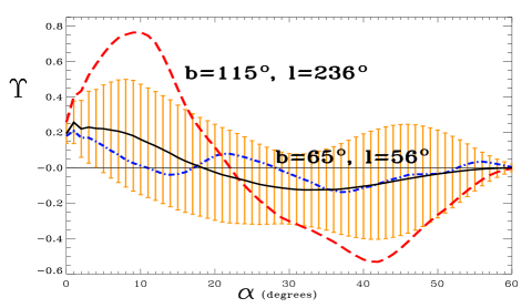
Figure 1: Plots of the difference histogram $\Upsilon(\alpha)$ illustrating the magnitudes of the deviation from isotropy as a function of separation angle calculated for two specific spherical caps, centered at $(b=65^{\circ},l=56^{\circ})$ and $(b=115^{\circ},l=236^{\circ})$, with a $\gamma_{0}=30^{\circ}$ of aperture. Plotted also, as a continuous line, is the mean $\Upsilon$ corresponding to the set of spherical caps into which the sphere was subdivided, along with the corresponding two-standard deviation region as a shaded area. As can be seen, the measured anisotropy is significant in one cap [$(b=115^{\circ},l=236^{\circ})$] but not in the other.

To define this indicator, let $\Omega_{j}\equiv\Omega(\theta_{j},\phi_{j};\gamma_{0})\in S^{2}$ be a spherical cap, with an aperture of $\gamma_{0}$ degrees, centered at $(\theta_{j},\phi_{j})$, for $j=1,\ldots,N_{\mbox{caps}}$, where the union of the $N_{\mbox{caps}}$ caps covers the whole celestial sphere $S^{2}$. Define the scalar function $\sigma:\Omega_{j}\mapsto\cal{R}^{+}$, that assigns to the $j^{\,\rm{th}}-$cap, centered at $(\theta_{j},\phi_{j})$, a real positive number $\sigma_{j}$ given by the variance of the $\Upsilon$ (which has zero mean)

$$\sigma^{2}_{j}\equiv\frac{1}{N_{\mbox{bins}}}\sum_{i=1}^{N_{\mbox{\footnotesize bins}}}\Upsilon^{2}_{j}(\alpha_{i})\;,$$ (5)

where $\Upsilon_{j}\equiv\Upsilon(\theta_{j},\phi_{j})$ is the $\Upsilon$ for the cap centered at $(\theta_{j},\phi_{j})$.

To obtain a local directional indicator, we cover the celestial sphere with a number of evenly distributed spherical caps and then calculate $\sigma_{j}$ for each cap. The $\sigma_{j}$ obtained in this way for each cap can then be viewed as a measure of anisotropy in the direction of the center of that cap. Patching together the $\sigma$ values for each cap, we obtain the indicator $\sigma=\sigma(\theta,\phi)$ defined over the whole celestial sphere, which measures the deviation from isotropy as a function of direction $(\theta,\phi)$. In this way, $\sigma(\theta,\phi)$ gives a scalar directional measure of anisotropy over the celestial sphere.

Now, since $\sigma(\theta,\phi)$ is a discrete scalar function defined on $S^{2}$, we can further quantify the details of its anisotropy content, by expanding it in spherical harmonics in the form

$$\sigma(\theta,\phi)=\sum_{\ell=0}^{\infty}\sum_{m=-\ell}^{\ell}b_{\ell m}\,Y_{\ell m}(\theta,\phi)$$ (6)

and calculate the corresponding $\sigma$ power spectrum

$$D_{\ell}=\frac{1}{2\ell+1}\sum_{m}|b_{\ell m}|^{2}\;.$$ (7)

It then follows that, if a large-scale asymmetry is present in the original temperature distribution, it should significantly affect the $\sigma$–map on the corresponding angular scales (i.e. its lower multipoles).

To recapitulate the multiple steps involved in defining our indicator $\sigma$, we itemize the procedure below:

1. Generate a set of evenly distributed overlapping spherical caps;

2. For each cap, divide the set of pixels into a number of submaps $N_{\mbox{his}}$, each containing an equal number of pixels within a temperature range;

3. Calculate the PASH, $\Phi_{\mbox{obs}}$, for each submap;

4. Average over all the $\Phi_{\mbox{obs}}$ for each cap to obtain $\langle\Phi_{\mbox{obs}}\rangle$;

5. Obtain the difference histogram $\Upsilon$ for each cap by subtracting $\Phi_{\mbox{exp}}-\langle\Phi_{\mbox{obs}}\rangle$;

6. Calculate the $\sigma$ value, using Eq. (5), for each cap;

7. Define the $\sigma$–map as the discrete function $\sigma(\theta,\phi)$ on $S^{2}$ where $\theta$ and $\phi$ are the coordinates of the center of each cap;

8. Calculate the multipoles $D_{\ell}$ for the $\sigma$–map.

From the above construction of $\sigma(\theta,\phi)$ and its power spectrum, it is clear that there is no direct relation between the temperature multipoles and the $\sigma(\theta,\phi)$ multipoles. Although they are implicitly related, the relation is likely to be very complicated. In this work we take a more pragmatic approach by treating our new anisotropy indicator as complementary to the usual temperature-based indicators, without attempting to establish a direct connection between them.

In the next section we shall apply the indicator $\sigma(\theta,\phi)$ to both the first and three-year WMAP data.

3 Application to WMAP data

The WMAP measurements have produced high angular resolution maps of the temperature field of the CMB. Here we considered both the first-year and the three-year WMAP data. For the first-year data we employed the full-sky foreground-cleaned Lagrange-ILC (LILC) map (Eriksen et al. 2004b ), the TOH map (Tegmark et al. TOH03 (2003)), as well as the coadded WMAP map (Hinshaw et al. Hinshaw03 (2003)). In all cases we chose HEALPix parameter $N_{\mbox{side}}=128$ (Górski et al. Gorski (2005)), corresponding to a partition of the celestial sphere into 196608 pixels. For the three-year WMAP data we used the coadded map and the foreground-cleaned maps ILC (Hinshaw et al. Hinshaw06 (2006)), OT (de Oliveira-Costa & Tegmark OT06 (2006)), and PPG (Park et al. PPG06 (2006)).

In all, we performed the $\sigma$–map analysis for seven CMB temperature maps: three using the first-year data and four with the full three-year data, all with different foreground cleaning algorithms. However, since the results are largely similar, we only present a detailed analysis of the three-year WMAP ILC map in the following. We also present the $\sigma$–maps for four of the remaining maps for comparison (the other two are similar to the depicted maps and were dropped to avoid repetition).

In our calculations of the $\sigma$–map for these CMB maps, we subdivided the sphere into a set of $N_{\mbox{caps}}=12288$ spherical caps of radius $30^{\circ}$ co-centered with the same number of pixels generated by HEALPix with $N_{\mbox{side}}=32$. We subdivided each cap into $N_{\mbox{his}}=64$ submaps, each consisting of the same number of pixels, and the number of bins chosen to produce the PASHs was taken to be $N_{\mbox{bins}}=180$.

Figure 2 shows the Mollweide projection of the $\sigma$–map in galactic coordinates obtained from the ILC WMAP map.

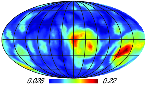
Figure 2: The full sky map of $\sigma(\theta,\phi)$ calculated from 12288 evenly distributed $30^{\circ}$ caps covering the ILC map.

As can be seen, the $\sigma$–map shows a high–$\sigma$ region suggestive of a dipole-like distribution. This result indicates that the distribution of hot and cold temperature pixels are not evenly distributed in the celestial sphere. We note that this is different from a temperature dipole, where one half of the sky would, on average, be hotter than the other. An anisotropy $\sigma$-dipole is not directly related to the temperature dipole, which was removed in all the CMB maps we have used, but is instead a result of large-angle anisotropies that are not readily apparent from a simple inspection of the temperature map alone. Particularly prominent is a very high–$\sigma$ region concentrated on the south eastern corner of the $\sigma$–map with a well-defined maximum at $(b=108^{\circ},l=222^{\circ})$. This is within a $16.6^{\circ}$ separation from the directions recently indicated by Eriksen et al. (2004a ) and Land & Magueijo (2005a ).

To obtain more quantitative information about the observed anisotropy, we calculated the power spectrum of the $\sigma$–map for the ILC map, which is represented by solid dots in Fig. 3.

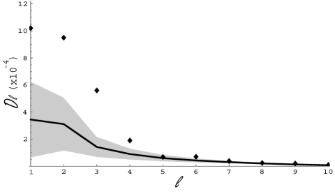
Figure 3: The power spectrum of the $\sigma$–map for the ILC map, for $\ell=1,\cdots,10$ (solid dots). Note the high values of the first three multipoles. For comparison, the mean expected power spectrum of the $\sigma$–map obtained by averaging over a set of 1000 Monte Carlo-generated, statistically isotropic CMB maps (solid curve). Shown also are the corresponding cosmic variance bounds for $\sigma$–maps (shaded area).

To estimate the statistical significance of these $\sigma$–multipole values, we compared the power spectrum of the $\sigma$–map, calculated for the ILC map, with the averaged power spectrum of the $\sigma$–map obtained by averaging over a set of 1,000 Monte Carlo-generated statistically isotropic CMB maps. Considering the WMAP best-fitting angular power spectrum of the $\Lambda$CDM model (Spergel et al. Spergel06 (2006)), each Monte Carlo CMB map is a stochastic realization of this spectrum obtained through randomized multipole components $a_{\ell m}$ generated within the cosmic variance limits.

The $\ell$ values used in this comparison lie in the range $1\leq\ell\leq 10$, which are sufficient to allow the investigation of the large-scale angular correlations corresponding to angular separations $\gtrsim 18^{\circ}$ in the $\sigma$–map. Moreover, we observe that $D_{\ell}\simeq 0$ for $\ell\geq 8$. Averaging over the 1,000 spectra of the $\sigma$–maps obtained from the Monte Carlo CMB maps gives the expected power spectrum, which is depicted in Fig. 3 (continuous line) along with the corresponding cosmic variance (shaded area).

We note that the very high dipole value (corresponding to $\ell=1$) found here is consistent with the $\sigma$–map (see Fig. 2) showing a clear separation of the higher and lower values for $\sigma$ into roughly two hemispherical regions. Using a $\chi^{2}$ test we have found this high value of the dipole to be statistically significant at $97\%$ confidence level, compared to the expected isotropic power spectrum. Note also the high values of the quadrupole and octopole moments that were found to be significant at $99\%$ and over $99.9\%$ (corresponding to a likelihood of one part in $10^{4}$ in a statistically isotropic map), respectively. We also find that the likelihood of the first three multipoles of an isotropically-generated map to have such high values simultaneously is very small being less than one part in $10^{5}$. Of the subsequent multipoles, only $D_{4}$ and $D_{6}$ fall outside the cosmic variance bounds.

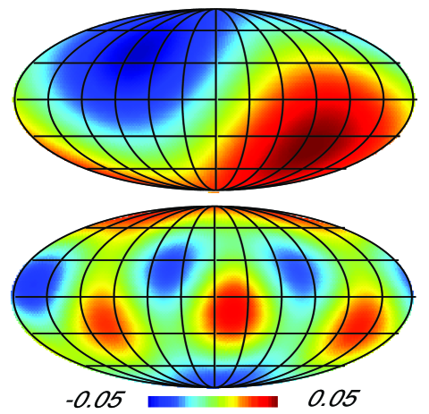
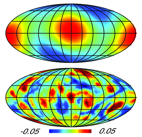
Figure 4: Depicted clockwise are the ILC $\sigma$–map’s dipole, quadrupole, octopole, and the remaining $\sigma$–map from which all these components plus the monopole were removed.

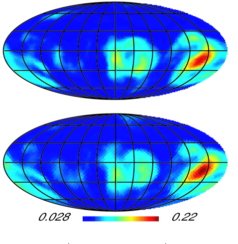
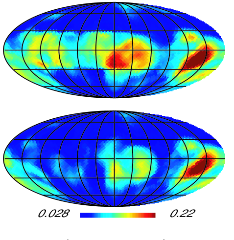
Figure 5: Depicted clockwise are the $\sigma$–maps: LILC, three-year coadded map (showing the effects of the unfiltered galactic contamination), OT and TOH WMAP maps. The one-year coadded and the PPG maps are not shown as they are very similar to the three-year coadded and the ILC maps, respectively. Note the high–$\sigma$ region in the south eastern corner of the $\sigma$–maps, which remains robust for all maps.

To check the robustness of our results we also calculated the power spectrum $\sigma$–map obtained from the WMAP PPG map. We found that the first three multipoles remain high relative to what would be expected from an isotropic case, at above $97\%$ statistical significance.

Given the anisotropic nature of the calculated $\sigma$–map, it is worth analyzing the shape of the anomalous multipoles in more detail. To this end, we depict in Fig. 4 the dipole, the quadrupole, and the octopole, as well as the full $\sigma$–map with these three components and the monopole removed. The analysis of the dipole alone gives a direction towards $(b=130^{\circ},l=259^{\circ})$, which on its own does not agree very well with the axis of maximum asymmetry found by Eriksen et al. (2004a ) and also by Land & Magueijo (2005a ). However, the sum of the first three multipoles has two maxima, one close to the galactic center, at $(b=97^{\circ},l=342^{\circ})$ and probably due to unremoved foregrounds, and the other in the direction $(b=112^{\circ},l=217^{\circ})$, which is in much better agreement with the axis of maximum asymmetry indicated by Eriksen et al. (2004a ) and Land & Magueijo (2005a ).

The quadrupole component has a very peculiar shape. It has two maxima and two minima lying symmetrically along a great circle. To determine this feature more precisely, we used the method proposed by de Oliveira-Costa et al. (OT03 (2003)), where for each given multipole (in their case, of the temperature map) the direction for which ‘angular momentum dispersion’ is maximized is said to be a preferred direction. Applying this to the $\sigma$–map, we find that the angular momentum dispersion for the quadrupole component is maximized in the direction $(b=80^{\circ},\,l=316^{\circ})$.

The calculation of our anisotropy indicator requires not only the choice of a CMB map as input, but also the specification of a number of ingredients and parameters whose choice could in principle affect the outcome of our results. To test the robustness of our scheme, hence of our results, we studied the effects of changing various parameters employed in the calculation of our indicator. We found that so long as the statistical noise (see Bernui and Villela BernuiVillela05 (2006)) satisfies

$$\frac{\sqrt{N_{\mbox{bins}}}}{n\sqrt{N_{\mbox{his}}}}\lesssim 0.05,$$ (8)

where $N_{\mbox{his}}$ is the number of submaps and $n$ is the mean number of pixels in each submap, then the $\sigma$–map and its power spectrum do not change appreciably as we change the number of submaps $N_{\mbox{his}}$ from 2 to 64, the size of the spherical caps between $15^{\circ}$ and $30^{\circ}$, the number of spherical caps, $N_{\mbox{caps}}$ (with values 768, 3072, and 12288, corresponding to HEALPix parameter $N_{\mbox{side}}=8,16$, and $32$, respectively) and the $N_{\mbox{bins}}$ values in the range 180 to 400.

Given that galactic foregrounds are likely to leave their most pronounced effects in the neighborhood of the galactic equator, one may suspect that the pronounced features, such as the high $\sigma$ region in the south eastern corner of the $\sigma$–map (see Fig. (2)), may be an artifact of the foreground contamination processes.

To show that this not the case, we first note that the latter feature lies outside the exclusion region defined by the Kp0 mask, which is the severest cut-sky WMAP mask. To proceed, we also calculated the $\sigma$–maps for the other 6 CMB temperature maps. We studied the three-year (Hinshaw et al. Hinshaw06 (2006)) and one-year coadded (Hinshaw et al. Hinshaw03 (2003)) maps, which are the combination of eight (from Q1 trough W4) foreground-reduced sky-maps in the Q–, V–, and W–bands, and minimized but did not seek to eliminate the galactic contamination. We also studied the foreground-cleaned TOH and OT maps given by Tegmark et al. (TOH03 (2003)) and de Oliveira-Costa & Tegmark (OT06 (2006)), as well as the LILC (Eriksen et al. 2004b ) and PPG (Park et al. PPG06 (2006)) CMB maps. The corresponding $\sigma$–maps are shown in Fig. 5 (the PPG and one-year coadded maps were dropped to avoid repetition). Together, these figures show that, despite differences in detail, the prominent high–$\sigma$ region in the south eastern corner remains robust.

These results indicate that the main anisotropic feature we have found is independent of the foreground cleaning processes employed. In addition we recently (Mota et al. MBRT2007 (2007)) performed a similar analysis of the WMAP one-year LILC data with both Kp0 and Kp2 masks applied and found very similar results. We also showed that this feature remains essentially the same in the Q, V and W bands (when analyzed after applying the Kp2 mask) which would not be expected if it were an artifact of uncleaned galactic foreground.

We should also note that apart from the high $\sigma$ region in the south eastern corner, which lies outside the Kp0 mask, there is another weaker structure around the galactic center. Although this structure remains in some form in all the maps we have analyzed its intensity and other details vary considerably for different choices of the cleaning algorithms, as can be seen from Figs. 2 and 5. Considering that it lies in the most contaminated region of the galactic plane, well inside the Kp0 mask, it is not clear whether this feature is not the result of the galactic foreground contamination. Furthermore its contributions to the excess dipole, quadrupole, and octopole is relatively minor compared to the high–$\sigma$ region in the south-eastern corner.

4 Conclusions

We have proposed a new method of measuring directional deviations from statistical isotropy in the CMB sky, in order to study the possible presence and nature of large-scale anisotropy in the WMAP data.

Our anisotropy indicator has enabled us to construct a $\sigma$–map in order to search for evidence of large-angle anisotropies in the WMAP CMB temperature field. In particular we have found, with high statistical significance, a small region in the celestial sphere with very high values of $\sigma$, indicative of an axis of asymmetry that defines a direction close to the one reported recently (Eriksen et al. 2004a ; Land & Magueijo 2005a ).

To obtain a more quantitative measure of this anisotropy, we studied the spherical harmonic expansion of the $\sigma$–map generated from the ILC map and found that the corresponding dipole component is significantly higher than would be expected, as compared with an average of a set of $\sigma$–maps obtained from 1000 Monte Carlo CMB maps generated under the statistical isotropy hypothesis. Moreover, we have found that the combination of the dipole, quadrupole, and octopole components of the $\sigma$–map has a strongly preferred direction close to the small region of the maximum value of $\sigma$.

Using a $\chi^{2}$ test we found that this high value of the dipole is statistically significant at a $97\%$ confidence level (CL), compared to the expected isotropic case. We also found high values of the quadrupole and octopole moments, which were found to be significant at $99\%$ CL and over $99.9\%$ CL (corresponding to a likelihood of one part in $10^{4}$ for statistically isotropic generated maps) respectively. The likelihood of the first three multipoles of an isotropically generated map to have such high values simultaneously is very small at less than one part in $10^{5}$.

We have shown that the results reported here are robust by showing that the $\sigma$–map does not significantly change with different choices of parameters, so long as the statistical noise is kept under control. We have also studied the effects of different foreground-cleaning algorithms, or absence thereof, by considering the LILC (first-year), TOH (first-year), OT (three-years), PPG (three-year), and the coadded (first and three-year) CMB maps in addition to WMAP three-year ILC map.

We have found again that the corresponding $\sigma$–maps remain qualitatively unchanged, in that the high–$\sigma$ region in the south eastern corner of the $\sigma$–map remains essentially invariant for all the maps considered here, while similar statistical significances for the most important (low-$\ell$) multipoles $D_{\ell}$ hold for all CMB maps considered. This provide evidence that our results regarding the large-angle anisotropy in the CMB maps remain unchanged no matter whether the first or three-year data are used.

This robustness demonstrates that our indicator is well-suited to the study of anisotropies in the CMB data. Furthermore, although derived from the temperature maps, it reveals features that are not apparent in the analysis of the temperature maps alone. Our scheme for studying directional anisotropies is complementary to the existing approaches in the literature, in the sense that it reveals different aspects of the same data set. However, the relationship between them is clearly non-trivial and requires further investigation, which is beyond the scope of the present work.

Regarding the origin of such large-angle anisotropy, a number of suggestions have been put forward. Briefly, they can arise either from a subtle form of unremoved foreground contamination (in which case the $\sigma$–map might indicate where in the sky this contamination is most intense) or from the universe being genuinely anisotropic on large angular scales. This possibility is particularly interesting, as it would have potentially important consequences for the standard inflationary picture, which predicts statistically isotropic CMB temperature fluctuation patterns.

Among this type of suggestions, it has been proposed that the preferred direction could be due to the universe possessing a non-trivial topology (see, e.g., Copi et al. Copi05 (2005); Spergel et al. Spergel03 (2003); for more details on cosmic topology see, e.g., the review articles Lachièze-Rey & Luminet CosmTopReviews (1995); Starkman Starkman (1998); Levin Levin (2002); Rebouças & Gomero RG (2004); Lehoucq et al. TopSign (1996); Roukema & Edge Roukema (1997); Cornish et al. Cornish (1998); Bond et al. 2000a ; 2000b ; Fagundes & Gausmann Fagundes (1999); Uzan et al. Uzan (1999); Gomero et al. Gomero00 (2000); 2001a ; 2001b ; 2001c ; Gomero02 (2002); Mota et al. Mota03 (2003, 2004); Luminet et al. Luminet03 (2003); Aurich et al. 2005a ; 2005b ; Hipolito-Ricaldi & Gomero Hipolito (2005); Weeks et al. 2003a ; Weeks 2003b ). If topology is indeed the origin, our anisotropic indicator is promising for distinguishing between different topologies. On the other hand, the extent to which this is true for the $\sigma$-indicator is unclear and deserves further investigation.

Whatever the origin of these large-angle anomalies may be, the robustness of our anisotropy indicator seems to be sufficiently sensitive to reliably map them, which in turn could facilitate the task of explaining their origin.

- (1) Abramo, L. R., Bernui, A., Ferreira, I., Villela, T., & Wuensche, C. A. 2006, Phys. Rev. D, 74, 063506
- (2) Aurich, R., Lustig, S., & Steiner, F. 2005a, Class. Quantum Grav., 22, 2061
- (3) Aurich, R., Lustig, S., & Steiner, F. 2005b, Class. Quantum Grav., 22, 3443
- (4) Bennett, C. L., Halpern, M., Hinshaw, G., et al. 2003a, ApJS, 148, 1
- (5) Bennett, C. L., Bay, M., Halpern, M., et al. 2003b, ApJ, 583, 1
- (6) Bernui, A., Tsallis, C., & Villela, T. 2006, Phys. Lett. A, 356, 426
- (7) Bernui, A. & Villela, T. 2006, A&A, 445, 795
- (8) Bernui, A., Villela, T., Wuensche, C. A., Leonardi, R., & Ferreira, I. 2006, A&A, 454, 409
- (9) Bielewicz, P., Eriksen, H. K., Banday, A. J., Górski, K. M., & Lilje, P. B. 2005, astro-ph/0507186
- (10) Bond, J. R., Pogosyan, D., & Souradeep, T. 2000a, Phys. Rev. D, 62, 043005
- (11) Bond, J. R., Pogosyan, D., & Souradeep, T. 2000b, Phys. Rev. D, 62, 043006
- (12) Bunn, E. F. & Scott, D. 2000, MNRAS, 313, 331
- (13) Chiang, L.-Y., Naselsky, P. D., Verkhodanov, O. V., & Way, M. J. 2003, ApJ, 590, L65
- (14) Coles, P., Dineen, P., Earl, J., & Wright, D. 2004, MNRAS, 350, 983
- (15) Cooray, A. & Seto, N. 2005, astro-ph/0509039
- (16) Copi, C. J., Huterer, D., & Starkman, G. D. 2004, Phys. Rev. D, 70, 043515
- (17) Copi, C. J., Huterer, D., Schwarz, D. J., & Starkman, G. D. 2005, astro-ph/0508047
- (18) Copi, C. J., Huterer, D., Schwarz, D. J., & Starkman, G. D. 2006, astro-ph/0605135
- (19) Cornish, N.J., Spergel, D., & Starkman, G. 1998, Class. Quantum Grav., 15, 2657
- (20) de Oliveira-Costa, A., Tegmark, M., Zaldarriaga, M., & Hamilton, A. 2004, Phys. Rev. D, 69, 063516
- (21) de Oliveira-Costa, A. & Tegmark M. 2006, Phys. Rev. D, 74, 023005
- (22) Donoghue, E. P. & Donoghue, J. F. 2005, Phys. Rev. D, 71, 043002
- (23) Eriksen, H. K., Hansen, F. K., Banday, A. J., Górski, K. M., & Lilje, P. B. 2004a, ApJ, 605, 14
- (24) Eriksen, H. K., Banday, A. J., Górski, K. M., & Lilje, P. B. 2004b, ApJ, 612, 633
- (25) Eriksen, H. K., Banday, A. J., Górski, K. M., & Lilje, P. B. 2005, ApJ, 622, 58
- (26) Fagundes, H. V. & Gausmann, E. 1999, Phys. Lett. A, 261, 235
- (27) Gomero, G. I., Rebouças, M. J., & Teixeira, A. F. F. 2000, Phys. Lett. A, 275, 355
- (28) Gomero, G. I., Rebouças, M. J., & Teixeira, A. F. F. 2001a, Class. Quantum Grav., 18, 1885
- (29) Gomero, G. I., Rebouças, M. J., & Tavakol, R. 2001b, Class. Quantum Grav., 18, 4461
- (30) Gomero, G. I., Rebouças, M. J., & Tavakol, R. 2001c, Class. Quantum Grav., 18, L145
- (31) Gomero, G. I., Teixeira, A. F. F., Rebouças, M. J., & Bernui, A. 2002, Int. J. Mod. Phys. D, 11, 869
- (32) Gordon, C., Hu, W., Huterer, D., & Crawford, T. 2005, astro-ph/0509301
- (33) Górski, K. M., Hivon, E., Banday, A. J., et al. 2005, ApJ, 622, 759
- (34) Hajian, A. & Souradeep, T. 2003, ApJ, 597, L5
- (35) Hajian, A., Souradeep, T., & Cornish, N. 2004, ApJ, 618, L63
- (36) Hajian, A. & Souradeep, T. 2005, astro-ph/0501001
- (37) Hansen, F. K., Banday, A. J., & Górski, K. M. 2004, MNRAS, 354, 641
- (38) Hansen, F. K., Cabella, P., Marinucci, D., & Vittorio, N. 2004, ApJ, 607, L67
- (39) Hinshaw, G., Spergel, D. N., Verde, L., et al. 2003, ApJS, 148, 135
- (40) Hinshaw, G., Nolta, M. R., Bennett, C. L., et al. 2006, astro-ph/0603451
- (41) Hipolito-Ricaldi, W. S. & Gomero, G. I. 2005, Phys. Rev. D, 72, 103008
- (42) Komatsu, E., Kogut, A., Nolta, M., et al. 2003, ApJS, 148, 119
- (43) Lachièze-Rey, M. & Luminet, J.-P. 1995, Phys. Rep, 254, 135
- (44) Land, K. & Magueijo, J. 2005a, MNRAS, 357, 994
- (45) Land, K. & Magueijo, J. 2005b, Phys. Rev. Lett., 95, 071301
- (46) Larson, D. L. & Wandelt, B. D. 2004, ApJ, 613, L85
- (47) Lehoucq, R., Lachièze-Rey, M., & Luminet, J.-P. 1996, A&A, 313, 339
- (48) Levin, J. 2002, Phys. Rep, 365, 251
- (49) Luminet, J.-P., Weeks, J. R., Riazuelo, A., Lehoucq, R., & Uzan, J.-P. 2003, Nature, 425, 593
- (50) Mota, B., Gomero, G. I., Rebouças, M. J., & Tavakol, R. 2004, Class. Quantum Grav., 21, 3361
- (51) Mota, B., Rebouças, M. J., & Tavakol, R. 2003, Class. Quantum Grav., 20, 4837
- (52) Mota, B., Bernui, A., Rebouças, M. J., & Tavakol, R. 2007, to appear in the Proceedings of the Second International Workshop on Astronomy and Relativistic Astrophysics, Int. J. Mod. Phys. D, in press.
- (53) Naselsky, P. D., Chiang, L.-Y., Olesen, P., & Verkhodanov, O. V. 2004, ApJ, 615, 45
- (54) Park, C.-G. 2004, MNRAS, 349, 313
- (55) Park, C.-G., Park, C., & Gott III, J. R. 2006, astro-ph/0608129
- (56) Prunet, S., Uzan, J.-P., Bernardeau, F., & Brunier, T. 2005, Phys. Rev. D, 71, 083508
- (57) Souradeep, T. & Hajian, A. 2004, Pramana, 62, 793
- (58) Souradeep, T. & Hajian, A. 2005, astro-ph/0502248
- (59) Teixeira, A. F. F. 2003, physics/0312013
- (60) Tomita, K. 2005, astro-ph/0509518
- (61) Rebouças, M. J. & Gomero, G. I. 2004, Braz. J. Phys., 34, 1358
- (62) Roukema B. F. & Edge A. 1997, MNRAS, 292, 105
- (63) Schwarz, D. J., Starkman, G. D., Huterer, D., & Copi, C. J. 2004, Phys. Rev. Lett., 93, 221301
- (64) Spergel, D. N., Verde, L., Peiris, H. V., et al. 2003, ApJS, 148, 175
- (65) Spergel, D. N., Bean, R., Doré, O., et al. 2006, astro-ph/0603449
- (66) Starkman, G. D. 1998, Class. Quantum Grav., 15, 2529
- (67) Tegmark, M., de Oliveira-Costa, A., & Hamilton, A. J. S. 2003, Phys. Rev. D, 68, 123523
- (68) Uzan, J.-P., Lehoucq, R., & Luminet, J.-P. 1999, A&A, 351, 766
- (69) Vale, C. 2005, astro-ph/0510137
- (70) Vielva, P., Martínez-González, E., Barreiro, R. B., Sanz, J. L., & Cayon, L. 2004, ApJ, 609, 22
- (71) Weeks, J. R., Lehoucq, R., & Uzan, J.-P. 2003a, Class. Quantum Grav., 20, 1529
- (72) Weeks, J. R. 2003b, Mod. Phys. Lett. A, 18, 2099
- (73) Weeks, J. R. 2004, astro-ph/0412231
- (74) Wiaux, Y., Vielva, P., Martínez-González, E., & Vandergheynst, P. 2006, Phys. Rev. Lett., 96, 151303, astro-ph/0603367
- (75) Wibig, T. & Wolfendale, A. W. 2005, MNRAS, 360, 236