Dimensional Analysis applied to Spectrum Handling in Virtual Observatory Context

The handling of units in an automated way by software systems can be a cumbersome procedure when the units are parsed as strings. Software systems parsing units have to take into account extensive tables of unit names, not always identical between different standards. In the Virtual Observatory context, the transfer of metadata in access protocols is specially critical for the understanding of the content of the data (many of which are legacy data). Driven by this issue, we present a way to handle units automatically which is based in dimensional analysis considerations. Although the approach presented here can be valid to any other branch of physics, we concentrate mainly in the application to spectrum handling in the VO context, and show how the proposed solution has been implemented in the VOSpec, a tool to handle VO-compatible spectra.

1 Introduction

Handling of units in spectra can be cumbersome when dealing with different Flux energy densities. For instance, the conversion between $F_{\lambda}$ and $F_{\nu}$ is normally done by parsing the unit name strings. Despite several efforts to homogenize unit name strings (See Greisen et al. (2004), Taylor (1995), George et al. (1995)), several different standards do exist, forcing the parsing-string mechanism to stick to one or several of those standards. On top of this, the adaptation of already existing legacy data to one or other standard might be a cumbersome -and even sometimes impossible- task.

The aforementioned problems led us to try and figure out a way to automatically handle units without the necessity to parse strings. Using dimensional analysis, we have devised an algorithmic way to convert between dimensionally homogeneous quantities. As a simple example, the string-parsing algorithm needed to convert between $W/cm^{2}/\mu m$ and $erg/cm^{2}/s/\AA$ (both $F_{\lambda}$) would be substituted for an algorithm to go from $10^{10}ML^{-1}T^{-3}$ to $10^{7}ML^{-1}T^{-3}$, i.e., dividing by a factor of $10^{3}$.

In section 2 we give a general mathematical formalism of the relevant parts of Dimensional Analysis techniques that will be needed for the handling of this problem. In this section we will follow with very slight modifications the excellent book by Szirtes (1997). We also describe the handling of the dimensional matrix to unveil how to extract dimensional relations between different units on the same problem. In section 3 we apply the theory to the case of $F_{\lambda}$ and $F_{\nu}$ conversions. And in section 4, we give a general algorithmic method for the conversion between different unit systems for the case of spectra together with details about the use of this technique in the VOSpec, a tool to handle SSAP (Simple Spectrum Access Protocol) compatible spectra developed at the European Space Astronomy Centre (ESAC) of the European Space Agency.

2 Dimensional Analysis overview

Dimensional analysis helps in the understanding of certain problems for which no analytic mathematical formulation exists, or for which the mathematical formulation is too complex. In these cases, the dimensional analysis allows to extract certain conclusions about the behavior of the system without the need of specific mathematical formulae relating the different variables of the problem at hand.

In physics we deal with quantities which have certain dimensions. These are combinations of a reduced number of basic or fundamental dimensions. These fundamental dimensions form a dimensional system. Dimensional systems can range from mono-dimensional (only a fundamental dimension is used to represent any physical quantity) to omni-dimensional (all dimensions are fundamental dimensions)(See ref Szirtes (1997) for examples). The intermediate, and mostly used, is the multidimensional system, in which a reduced set of fundamental dimensions is used. In the examples that will follow, we will adhere to the most widely used system of MASS-LENGTH-TIME system with the addition of Temperature, Electric current and luminosity to deal with other more complex problems. Following a long tradition in dimensional analysis (see Maxwell (1890)) will call M-L-T these fundamental dimensions. Following this convention, a physical quantity, e.g., a Force, would be represented as follows:

$[F]=[m][a]=MLT^{-2}$

where square brackets should be read as ”dimensions of” and we will call the rightmost part the ”dimensional equation” of the quantity under consideration.

2.1 Dimensional Matrix

Let $F(V_{1},V_{2},...,V_{n})=0$ be a physical relation among a set of variable quantities $V_{i}$. The dimensional equations of the different variables will be:

$$[V_{1}] = d_{1}^{\alpha_{11}}d_{2}^{\alpha_{12}}...d_{n}^{\alpha_{1n}}$$

$$\left[V_{2}\right] = d_{1}^{\alpha_{21}}d_{2}^{\alpha_{22}}...d_{n}^{\alpha_{2n}}$$

$$...$$

$$\left[V_{n}\right] = d_{1}^{\alpha_{m1}}d_{2}^{\alpha_{m2}}...d_{n}^{\alpha_{mn}}$$

The matrix formed with the exponents of the dimensions is called the Dimensional Matrix:

$$\mathbf{D}=\left[\begin{array}[]{cccc}\alpha_{11}&\alpha_{12}&\ldots&\alpha_{1n}\\ \alpha_{21}&\alpha_{22}&\ldots&\alpha_{2n}\\ \vdots&\vdots&\ldots&\vdots\\ \alpha_{m1}&\alpha_{m2}&\ldots&\alpha_{mn}\end{array}\right]$$ (1)

From the dimensional matrix, we can now tackle the following problem: how can we find dimensional (or dimensionless) products of the variables at hand?. In other words, how do we find the $\varepsilon_{1},\varepsilon_{2},...,\varepsilon_{n}$ exponents that solve the following equation:

$$[V_{1}^{\varepsilon_{1}}V_{2}^{\varepsilon_{2}}...V_{n}^{\varepsilon_{n}}]=d_{1}^{q_{1}}d_{2}^{q_{2}}...d_{p}^{q_{p}}$$ (2)

where: $V_{1},...,V_{n}$ are the variables of the problem, $d_{1},...,d_{p}$ are the fundamental dimensions of the problem, $q_{1},...,q_{p}$ are the given exponents (sought combinations of fundamental dimensions; to be set equal to zero for dimensionless products).

The problem is therefore reduced to solving for $\varepsilon_{j}$ the following system of linear equations:

$$\sum_{j=1}^{n}\>D_{ij}\>\varepsilon_{j}\>=\>q_{i}$$ (3)

It can be shown that (see Szirtes (1997)) the solution to the above is:

$$\varepsilon_{j}\>=\>\sum_{k=1}^{n}\>E_{jk}\>\eta_{k}$$ (4)

where:

$$\mathbf{E}=\left[\begin{array}[]{cccc}\mathbf{1}&\vdots&\mathbf{0}\\ \ldots&&\ldots\\ -\mathbf{A^{-1}}\mathbf{B}&\vdots&\mathbf{A^{-1}}\end{array}\right]$$

and $\mathbf{A}$ is a nonsingular square matrix of size the rank of the dimensional matrix, and $\mathbf{B}$ is formed by the rest of columns included in $\mathbf{D}$ and not included in $\mathbf{A}$. The sizes of the different matrices are:

$$\begin{array}[]{rlr}\mathbf{E}:&(n)\times(n)&square\>matrix\\ \mathbf{I}:&(n-p)\times(n-p)&identity\>matrix\\ \mathbf{0}:&(n-p)\times(p)&null\>matrix\\ \mathbf{A}:&(p)\times(p)&square\>matrix\\ \mathbf{B}:&(p)\times(n-p)&\>matrix\\ \mathbf{A^{-1}B}:&(p)\times(n-p)&\>matrix\end{array}$$

the column matrix $\eta_{k}$ is formed by $\varepsilon_{n-p}$ arbitrary exponents followed by $q_{p}$ sought dimensional exponents. The first $\varepsilon_{n-p}$ are arbitrary due to the fact that $R_{D}\equiv rank(\mathbf{D})=p$ and therefore out of the n exponents we can only determine p, leaving n-p arbitrary. Therefore, $\eta_{k}$ is:

$$\eta_{k}=\left[\begin{array}[]{l}\varepsilon_{1}\\ \varepsilon_{2}\\ \vdots\\ \varepsilon_{n-p}\\ q_{1}\\ q_{2}\\ \vdots\\ q_{p}\end{array}\right]$$

The problem is thus reduced to finding the matrix $\mathbf{P}$ result of the product:

$$P_{ij}\>=\>\sum_{k=1}^{n}\>E_{ik}\>Z_{kj}\>$$ (5)

where $Eik$ is as defined earlier and $Z_{kj}$ is the result of superimposing the $\eta_{k}$ columns for the different variables:

$$\mathbf{Z}=\left[\begin{array}[]{cccc}\varepsilon_{11}&\varepsilon_{12}&\ldots&\varepsilon_{1p}\\ \varepsilon_{21}&\varepsilon_{22}&\ldots&\varepsilon_{2p}\\ \vdots&\vdots&\ldots&\vdots\\ \varepsilon_{(n-p)1}&\varepsilon_{(n-p)2}&\ldots&\varepsilon_{(n-p)p}\\ q_{1}&q_{1}&\ldots&q_{1}\\ q_{2}&q_{2}&\ldots&q_{2}\\ \vdots&\vdots&\ldots&\vdots\\ q_{p}&q_{p}&\ldots&q_{p}\end{array}\right]$$ (6)

both $\mathbf{P}$ and $\mathbf{Z}$ are of size nxp.

In the particular case where we are seeking for dimensionless products, all the $q_{i}$ will be set to zero (dimensional exponents) as a dimensionless quantity is considered to have dimension=1 (for a dissertation on the convenience to call dimensionless these type of quantities, check Szirtes (1997)).

2.2 Complete set of dimensional products: Buckingham theorem

The so called Buckingham’s theorem reads as follows:

The number of independent dimensional products $n_{\pi}$ which can be composed for a given number of variables and dimensions is:

$$\begin{array}[]{rlll}n_{\pi}&=&n\>-\>R_{D}&for\>dimensionless\>products\\ n_{\pi}&=&n\>-\>R_{D}\>+\>1&for\>dimensional\>products\end{array}$$

where $n$ is the number of variables and $R_{DM}$ is the rank of the dimensional matrix.

In this case, the sizes of the matrices at would be:

$$\begin{array}[]{rlr}\mathbf{I}:&(n-R_{D})\times(n-R_{D})&identity\>matrix\\ \mathbf{0}:&(n-R_{D})\times(R_{D})&null\>matrix\\ \mathbf{A}:&(R_{D})\times(R_{D})&square\>matrix\\ \mathbf{B}:&(R_{D})\times(n-R_{D})&\>matrix\\ \mathbf{E}:&(n)\times(n)&square\>matrix\\ \mathbf{A^{-1}B}:&(R_{D})\times(n-R_{D})&\>matrix\end{array}$$

An obvious advantage of finding the dimensionless products of the problem under investigation is that it reduces the number of parameters relevant to the system. In the case that the precise mathematical formula governing the behavior of the system is known, e.g., the Navier-Stokes equation for a fluid system, then the dimensionless products give information as well on the relative importance of each of the terms in the equation, helping in the simplification of the equations for certain combinations of the dimensionless products (for a beautiful example regarding the Navier-Stokes equations, see Diez-Roche (1980)).

3 Application to Spectral Fluxes

Using the dimensional analysis principles, we will extract the dimensionless products for flux densities. These products will be used later, in section 4, to achieve the unit conversion between flux densities in different units.

3.1 $F_{\lambda}$ versus $\lambda$

To construct the dimensional matrix for $F_{\lambda}$ we will consider a spectral energy distribution of the form:

$$F_{\lambda}(c,\lambda,h)=0$$ (7)

The dimensional equations of the different members of the previous relation are:

$$[F_{\lambda}]=ML^{-1}T^{-3},\;[c]=LT^{-1},\;[\lambda]=L,\;[h]=ML^{2}T^{-1}$$ (8)

we now construct the following table:

$$F_{\lambda}$$

M 1 0 0 1

L -1 1 1 2

T -3 -1 0 -1

(9)

according to previous sections, we will have the following set of matrices:

$$\mathbf{A}=\left[\begin{array}[]{rrr}0&0&1\\ 1&1&2\\ -1&0&-1\\ \end{array}\right]\hskip 56.9055pt\mathbf{B}=\left[\begin{array}[]{r}1\\ -1\\ -3\\ \end{array}\right]$$

$$\mathbf{-A^{-1}B}=\left[\begin{array}[]{r}-2\\ 5\\ -1\\ \end{array}\right]\hskip 56.9055pt\mathbf{E}=\left[\begin{array}[]{rrrr}1&0&0&0\\ -2&-1&0&-1\\ 5&-1&1&1\\ -1&1&0&0\\ \end{array}\right]$$

$$\mathbf{Z}=\left[\begin{array}[]{rrrr}1&1&1&1\\ 0&0&0&0\\ 0&0&0&0\\ 0&0&0&0\\ \end{array}\right]\hskip 14.22636pt\mathbf{P}=\mathbf{E}*\mathbf{Z}=\left[\begin{array}[]{rrrr}1&1&1&1\\ -2&-2&-2&-2\\ 5&5&5&5\\ -1&-1&-1&-1\\ \end{array}\right]$$

where following the general practice (see Szirtes (1997)) we have chosen the matrix A to be composed of the independent variables in relation (7), and he matrix $\mathbf{P}$ gives the exponents(columns) on the dimensions (rows) that give rise to dimensionless products. According to the theory before, the number of dimensionless products in this case would be $n-R_{DM}$, i.e., 4-3=1, hence the fact that three of the columns are linear combinations of the remaining one (identical, in this case) in the P matrix only giving result to one dimensionless product combination:

$$\begin{array}[]{lr}\mathbf{P}=\left[\begin{array}[]{rrrr}1&1&1&1\\ -2&-2&-2&-2\\ 5&5&5&5\\ -1&-1&-1&-1\\ \end{array}\right]&\end{array}$$

where rows identify the variables in (8) and columns correspond to the exponents of those variables.

Therefore, the unique dimensional product thus for this case would be:

$$\pi=F_{\lambda}\frac{\lambda^{5}}{c^{2}h}$$ (15)

3.2 $F_{\nu}$ versus $\lambda$

Following exactly the same procedure as before, we would have:

$$F_{\nu}$$

M 1 0 0 1

L 0 1 1 2

T -2 -1 0 -1

(16)

and therefore:

$$\mathbf{A}=\left[\begin{array}[]{rrr}0&0&1\\ 1&1&2\\ -1&0&-1\\ \end{array}\right]\hskip 56.9055pt\mathbf{B}=\left[\begin{array}[]{r}1\\ 0\\ -2\\ \end{array}\right]$$

$$\mathbf{-A^{-1}B}=\left[\begin{array}[]{r}-1\\ 3\\ -1\\ \end{array}\right]\hskip 56.9055pt\mathbf{E}=\left[\begin{array}[]{rrrr}1&0&0&0\\ -1&-1&0&-1\\ 3&-1&1&1\\ -1&1&0&0\\ \end{array}\right]$$

$$\mathbf{Z}=\left[\begin{array}[]{rrrr}1&1&1&1\\ 0&0&0&0\\ 0&0&0&0\\ 0&0&0&0\\ \end{array}\right]\hskip 14.22636pt\mathbf{P}=\mathbf{E}*\mathbf{Z}=\left[\begin{array}[]{rrrr}1&1&1&1\\ -1&-1&-1&-1\\ 3&3&3&3\\ -1&-1&-1&-1\\ \end{array}\right]$$

And therefore the only dimensionless product would be:

$$\pi^{\prime}=F_{\nu}\frac{\lambda^{3}}{ch}$$ (20)

Both dimensionless quantities in (15) and (20) are descriptions of the same physical problem. As they are lineal in the dependent variable ($F_{\lambda}$ and $F_{\nu}$ respectively) we are able to conclude that they will be equivalent, i.e., that we can write in this case:

$\pi=\pi^{\prime}$

and therefore:

$$F_{\lambda}\frac{\lambda^{5}}{c^{2}h}=F_{\nu}\frac{\lambda^{3}}{ch}\>\>\Longrightarrow\>\>F_{\lambda}=\frac{c}{\lambda^{2}}F_{\nu}$$ (21)

which is the physical result expected when transforming flux densities.

The dimensionless product obtained when repeating the above procedure for $F_{\nu}$ and $F_{\lambda}$ with $\nu$ as the independent variable give:

$$\pi=F_{\nu}\frac{c^{2}}{\nu^{3}h}\>\>\>\>\mbox{and}\>\>\>\>\>\pi=F_{\lambda}\frac{c^{3}}{\nu^{5}h}\>\>\>\mbox{respectively}$$

This working example shows how the dimensional analysis can be used in the handling of spectrum fluxes and unit transformation. Much more complex problems can be tackled using this approach. For a nice compilation of literally hundreds of examples, consult the book by Szirtes (1997).

In what follows, we give an algorithm to bring the aforementioned ideas to practice when designing a client tool to handle Virtual Observatory spectra.

3.3 Comment on apparent velocity as X-axis spectral coordinate

In the paper by Greisen et al. (2004), the apparent radial velocity is considered as one of the possible spectral coordinates. A whole set of possible transformations between the different spectral coordinates (”x-axes”) is given together with their derivatives. The paper deals spectral coordinate transformations, rather than with flux transformations (on the ”y-axis”). In this work, we deal with energy densities which depend, generally, on $\lambda$ or $\nu$.

Conversions in the x-axis to velocity space do need a central reference wavelength (frequency) which will have to accompany the metadata for the data. Once this value is known, the transformation of the x-axis will just consist of a translation plus a dilation, and the Y-axis will be kept as is. In the case that the data are coming with velocity in the x-axis, they will have to contain the reference lambda giving rise to those velocity values, and the process to convert the data to wavelength values would be simply inverted.

4 Algorithmic approach and use in VOSpec

In the Virtual Observatory context, there is a need to have a standard protocol to make spectra accessible from different projects in a simple way. The idea is to create a protocol for spectra in the same line as the already standard Simple Image Access Protocol (SIAP), that would allow for the creation of on-the-fly Spectral Energy Distributions (SEDs) from heterogeneous data sets.

This protocol has been called Simple Spectrum Access Protocol (SSAP) and basically implements a two-step process:

• In the first step, a cone search is done on available services and the match results are sent, together with metadata,  in a VO standard VOTable.

• In the second step, the pointers to the real data files (spectra) are called and data are retrieved.

The main problem faced when trying to create an SED using data from different projects/formats is to compare data different units. We should be able to transform spectral coordinate units and fluxes to a common unit system.

Our proposed solution is to specify in the metadata (first SSAP step) for every spectrum, the dimensional equation for the spectrum axes, and use dimensional analysis to extract the conversion formulae needed to go from one to the other.

To prove that this on-the-fly conversion was possible, we developed a tool called VOSpec, able to request different SSAP servers and produce a common SED from different spectra in different formats from different projects.

The application is already available to the general public at: http://esavo.esa.int/vospec/ and it has been used for the AVO demo which took place on Jan 25 & 26, 2005 at ESAC. See AVO Demo (2005) for reference.

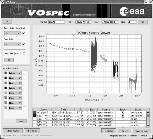
Figure 1: SED generated for the quasar 3c273 using VOSpec, covering from Radio to X-Ray spectral data. From left to right: Radio and sub-milimiter points (local files loaded data taken from the Geneve University database). Infrared spectrum data from the ISO SSAP service (LWS and PHOT data). Optical and ultraviolet spectrum data from FUSE (SSAP service) and HST(FOS) (SSAP service). On the right, X-Ray data from XMM-Newton (processed local file)

At the time of writing this paper, spectra from ISO, IUE, HST (FOS), SDSS, HyperLeda and FUSE projects are already providing SSAP access to their data. All the spectra from these services can be superimposed in the same display, and the user can generate on-the-fly SEDs as can be seen in Figure  1. Spectra from projects that don’t have SSAP services, can be loaded locally using the SSAP Wrapper Creator integrated in VOSpec.

4.1 Algorithmic approach

There are several ways to describe a spectrum flux and the spectral coordinate inside a 1-D spectrum. A conversion table could be used to make the transformations accordingly, but it is not easy to use in an automatic algorithm, and this would limit the number of possible transformations allowed by the system.

In this section, we will describe an algorithmic way to approach the units problem from the dimensional point of view and show how this is used in the VOSpec application.

A unit can be described in the following way:

$$[UNIT]=Scaling*M^{a}L^{b}T^{c}$$ (22)

where the scaling factor is defined with respect to a certain common system of units and the exponents a,b,c define the unit dimensionally. We will choose the SI as our base dimensional system of reference.

In order to understand how the algorithm works, suppose we are dealing with a spectrum in Jansky (y-axis) and Hertz (x-axis). The units dimensions (and scale factors) turn out to be:

$$\nu(Hz) = T^{-1}$$

$$F_{\nu}(Jy) = 10^{-26}MT^{-2}$$

where $1$ and $10^{-26}$ are the reference scaling factors to the SI units system for $Hz$ and $Jy$ respectively.

Suppose now, we want to convert one spectrum point defined by the pair $\left[\nu(Hz),F_{\nu}(Jy)\right]$ to other ones, e.g. $\left[\lambda(\mu m),F_{\lambda}(\frac{W}{cm^{2}\mu m})\right]$, i.e.:

$$\lambda(\mu m) = 10^{-6}L$$

$$F_{\lambda}(\frac{W}{cm^{2}\mu m}) = 10^{10}ML^{-1}T^{-3}$$

First we need to generate the matrix $E$ for the original system, as we saw in section 3:

$$F_{\nu}$$

M 1 0 0 1

L 0 1 0 2

T -2 -1 -1 -1

(23)

so, in this case:

$$\mathbf{A}=\left[\begin{array}[]{rrr}0&0&1\\ 1&0&2\\ -1&-1&-1\\ \end{array}\right]\hskip 14.22636pt\mathbf{A^{-1}}=\left[\begin{array}[]{rrr}-2&1&0\\ 1&-1&-1\\ 1&0&0\\ \end{array}\right]$$

and constructing $\mathbf{B}$ from the Flux density units:

$$\mathbf{B}=\left[\begin{array}[]{r}1\\ 0\\ -2\\ \end{array}\right]\hskip 14.22636pt\mathbf{-A^{-1}B}=\left[\begin{array}[]{r}2\\ -3\\ -1\\ \end{array}\right]$$

so finally, constructing the matrix $\mathbf{E}$ using the rules described in section 3:

$$\mathbf{E}=\left[\begin{array}[]{rrrr}1&0&0&0\\ 2&-2&1&0\\ -3&1&-1&-1\\ -1&1&0&0\\ \end{array}\right]$$

Now, to go from one system to the other, we have to generate two different Z matrices, one for the spectrum coordinate transformation and the second one for the flux transformation. As we are looking for certain target dimensions, the Z matrix will have to include the sought dimensional exponents, and therefore, as the final spectrum coordinates are $\mu m$ ($L$) we will have:

$$\begin{array}[]{lr}\mathbf{Z_{1}}=\left[\begin{array}[]{r}0\\ 0\\ 1\\ 0\\ \end{array}\right]&\begin{array}[]{rrrr}F_{\nu}\\ M\\ L\\ T\\ \end{array}\end{array}$$

where the first zero is imposing no dependence in the flux, and the rest are the exponents in $M$, $L$, $T$ respectively.

For the final system of units, the $F_{\lambda}$ is $\frac{W}{cm^{2}\mu m}$ ($ML^{-1}T^{-3}$):

$$\begin{array}[]{lr}\mathbf{Z_{2}}=\left[\begin{array}[]{r}1\\ 1\\ -1\\ -3\\ \end{array}\right]&\begin{array}[]{rrrr}F_{\nu}\\ M\\ L\\ T\\ \end{array}\end{array}$$

where, as it was defined in previous section, the first element is the dependence in the flux and the rest of the elements in the $Z$ are the dimensional equation exponents for $M$,$L$ and $T$ respectively.

If we multiply then the original E matrix with these Z vectors we obtain for the spectral coordinate:

$$\begin{array}[]{lr}\mathbf{P_{1}}=\mathbf{E*Z_{1}}=\left[\begin{array}[]{r}0\\ 1\\ -1\\ 0\\ \end{array}\right]&\begin{array}[]{rrrr}F_{\nu}\\ c\\ \nu\\ h\\ \end{array}\end{array}$$

and for the flux:

$$\begin{array}[]{lr}\mathbf{P_{2}}=\mathbf{E*Z_{2}}=\left[\begin{array}[]{r}1\\ -1\\ 2\\ 0\\ \end{array}\right]&\begin{array}[]{rrrr}F_{\nu}\\ c\\ \nu\\ h\\ \end{array}\end{array}$$

That means, respectively:

$$\left[\lambda\right] = \frac{\left[c\right]}{\left[\nu\right]}$$

$$\left[\frac{W}{cm^{2}\mu m}\right] = \left[Jy\right].\frac{\left[\nu\right]^{2}}{\left[c\right]}$$

To finalize the transformation, we must include the scaling factors of the different units. To achieve this goal, we note that every time a magnitude is used, the scaling must appear, i.e.,

$$S_{(\mu m)}\lambda(\mu m) = \frac{c}{S_{(Hz)}\nu(Hz)}$$

$$S_{(\frac{W}{cm^{2}\mu m})}F_{\lambda}(\frac{W}{cm^{2}\mu m}) = S_{(Jy)}F_{\nu}(Jy).\frac{(S_{(Hz)}\nu(Hz))^{2}}{c}$$

Where the S elements correspond to the scalings with respect to a common system of reference units (in this case SI).

Finally we obtain:

$$\lambda(\mu m) = \frac{1}{S_{(\mu m)}.S_{(Hz)}}.\frac{c(m/s)}{\nu(Hz)}$$

$$= 10^{6}.\frac{c(m/s)}{\nu(Hz)}$$

$$F_{\lambda}(\frac{W}{cm^{2}\mu m}) = \frac{S_{(Jy)}.S^{2}_{(Hz)}}{S_{(\frac{W}{cm^{2}\mu m})}}F_{\nu}(Jy)\frac{\nu^{2}(Hz)}{c(m/s)}$$

$$= \frac{10^{-26}}{10^{10}}F_{\nu}(Jy)\frac{\nu^{2}(Hz)}{c(m/s)}$$

$$= 10^{-36}F_{\nu}(Jy)\frac{\nu^{2}(Hz)}{c(m/s)}$$

These final formulae tell us how to express the values of a $\left[x,y\right]$ point in the final units as a function of the point in the original ones.

The algorithm can be summarized as follows:

1. Construct the matrix A, using the spectral coordinate, c and h dimensional equations.

2. Construct the vector B using the flux density dimensional equation.

3. Invert the matrix A, and construct the matrix E as it was described in point 1.

4. Construct two Z vectors using spectral coordinate and flux density dimensional equations of the final units.

5. Multiply the matrix E with the two Z vectors to obtain the conversion factors.

6. Finally, use the scaling factors to finish the conversion.

5 Conclusions

We have shown how to make use of Dimensional Analysis techniques to handle unit conversion in an automated way for the case of spectral flux densities.

We have proposed the IVOA to include the SCALEQ and DIMEQ parameters as part of the Simple Spectrum Access Protocol so that clients can use Dimensional Analysis algorithms to handle units automatically.

The approach shown is not only relevant to the Spectral access within the VO, and can be extended -as mentioned in the introduction- to any physical problem by including the relevant dimensions.

In this sense, we imagine any unit as composed of three main attributes:

1. A name (and possibly a symbol)

2. A SCALEQ (giving the Scaling of the unit with respect to the International System of Units)

3. A DIMEQ (giving the dimensions of the unit)

An example of a serialization of this units model could be the FITS representation, in which a unit like the ”Jansky” could be represented in the following way:

$$\begin{array}[]{lll}CUNIT=^{\prime}Jansky^{\prime}\\ CSCALEQ=^{\prime}1E-26^{\prime}\\ CDIMEQ=^{\prime}MT**-2^{\prime}\end{array}$$

Certainly, to cover all possible physical units, more dimensions than M-L-T would be needed, but the set will always be far smaller than the units they can represent.