Bulk viscous cosmology: statefinder and entropy

Abstract

The statefinder diagnostic pair is adopted to differentiate viscous cosmology models and it is found that the trajectories of these viscous cosmology models on the statefinder pair $s-r$ plane are quite different from those of the corresponding non-viscous cases. Particularly for the quiessence model, the singular properties of state parameter $w=-1$ are obviously demonstrated on the statefinder diagnostic pair planes. We then discuss the entropy of the viscous / dissipative cosmology system which may be more practical to describe the present cosmic observations as the perfect fluid is just a global approximation to the complicated cosmic media in current universe evolution. When the bulk viscosity takes the form of $\zeta=\zeta_{1}\dot{a}/a$($\zeta_{1}$ is constant), the relationship between the entropy $S$ and the redshift $z$ is explicitly given out. We find that the entropy of the viscous cosmology is always increasing and consistent with the thermodynamics arrow of time for the universe evolution. With the parameter constraints from fitting to the 157 gold data of supernova observations, it is demonstrated that this viscous cosmology model is rather well consistent to the observational data at the lower redshifts, and together with the diagnostic statefinder pair analysis it is concluded that the viscous cosmic models tend to the favored $\Lambda$CDM model in the later cosmic evolution, agreeable to lots of cosmological simulation results, especially to the fact of confidently observed current accelerating cosmic expansion.

I Introduction

Observations of type Ia supernova(SNe Ia) suggest that the expansion of the universe at later stage is in an accelerating phase. Additionally, the measurement of the cosmic microwave background (CMB) DNS and the galaxy power spectrum MT indicate that in spatially flat isotropic universe, about two-thirds of the critical energy density seems to be stored in a dark energy component (the simplest candidate is the famous cosmological constant $\Lambda$) with negative enough pressure AGR0 . Ironically, we do not know much about dark energy (DE) properties, if not less than those on the mysterious dark side of the universe sc .

In order to explore the implying accelerating mechanism, many authors propose a variety of models to describe the evolution of our universe, like the modified gravity xh for example. Among these and opposite to the extending Hilbert-Einstein action for general relativity modifications, there exist a class of models that are based on searching for a proper equation of state(EoS) for the matter-energy fluid. Initially, this class of models are exploited in the context of the perfect fluid. The viscosity concept is introduced into dark energy study relatively lately. And now it seems to play a more and more important and practical role in the more realistic cosmology model constructions. Other earlier attempts in this line can be found in referencesCWM ; SN ; IB ; IB1 ; IB2 ; TP . Additionally, for more details Grøn have given a very useful review for the subject in referenceG .

Viscosity is a concept in fluid mechanics related to velocity gradient and is divided into two classes, shear viscosity and bulk viscosity. In viscous cosmology, shear viscosity comes into play in connection with spacetime anisotropy. An analytic formula for the traceless part of the anisotropy stress tensor has been derived by S.WeinbergW . Meanwhile, a bulk viscosity usually functions in an isotropic universe. Under the Friedmann-Robertson-Walker (FRW) framework, the energy-momentum tensor at most has a bulk viscosity term as $T_{ik}=(p-\zeta\theta)g_{ik}$($\zeta$ is bulk viscosity, and $\theta$ is the expansion scalar). Additionally, bulk viscosity related to the grand-unified-theory phase transition PL may lead to explain the cosmic acceleration expansion.

At present, a large number of models exist but without very effective methods either verifying them or ruling them out. For this reason, there is a strong need for diagnostic techniques. The statefinder diagnostic pair $\{r,s\}$, which is purely geometric quantities introduced by Sahni, Saini, Starobinsky and AlamVS , provides us a very useful method to discriminate cosmological models. The statefinder pair probes the expansion dynamics of the universe through higher derivatives of the expansion factor $\dddot{a}$($a$ is the scale factor) which is a natural companion to the deceleration parameter that depends upon $\ddot{a}$. Different models on the $s-r$ plane accordingly show different trajectories. For example, the spatially flat $\Lambda$CDM scenario corresponds to a fixed point $\{0,1\}$ in the statefinder diagnostic pair $\{r,s\}$ plane, with which the ‘distance’ of other Dark Energy (DE) models from $\Lambda$CDM can therefore be established on the $s-r$ plane UA . Additionally, the statefinder pair has possessed the merits that can discriminate among a large amount of models including $\Lambda$CDM, quintessence, kinessence, Chaplygin gas(see references VS ; UA ; VG ; WZ ). With the introduction of new observational techniques and increasing improvement of measurement, it is certainly for us to get more precision data and richer information about the geometric quantities, with possibilities to evaluate more practical cosmology models, like those reasonable tries by considering viscosity to abandon the commonly used and simplest perfect fluid approximation to real cosmic media, and at that time some models would be either verified or ruled out by the statefinder diagnostic pair and other astrophysics observations. More reference about recent and future experiments can be found in the review paperSH .

This paper is arranged as follows: In Sec.II, the general formalism is presented for following discussions; In Sec.III, we discuss the difference between perfect fluid models and non-perfect fluid models from the viewpoint of density and trajectories of the diagnostic pair$\{r,s\}$, especially in Quiessence modelUA ; VG ; qm ; In Sec.IV, our attentions are focused on variable bulk viscosity dark energy model with general EoS. The entropy of system is deeply discussed there apart from statefinder pair diagnostics, as we have realized that the thermodynamics can reflect more important global characters for a complicated system, like our observable universe as shown by Brevik, Nojiri, Odintsov and Vanzoe in the reference IB2 . And the last section is devoted to our conclusions.

II General formalism

Now, we introduce the basic framework for our discussions. That is, in Friedmann-Robertson- Walker(FRW) cosmology the metric of the system is chosen as:

$$ds^{2}=-dt^{2}+a^{2}(\frac{dr^{2}}{1-kr^{2}}+r^{2}d\Omega^{2})$$ (1)

where $a$, and $k$ are the scale factor and space curvature, respectively. The Einstein equations take the usual form

$$G_{\mu\nu}=R_{\mu\nu}-\frac{1}{2}Rg_{\mu\nu}=8\pi GT_{\mu\nu}$$ (2)

Note that we have included the cosmological constant $\Lambda$ in the energy-momentum tensor $T_{\mu\nu}$. In the FRW cosmology with bulk viscosity, the stress-energy-momentum tensor is written as:

$$T_{\mu\nu}=(\rho+p)U_{\mu}U_{\nu}+pg_{\mu\nu}-\zeta\theta h_{\mu\nu}$$ (3)

where $\zeta$ is the bulk viscosity, $\theta$ the expansion factor defined by $\theta=U^{\mu}_{;\mu}=3\dot{a}/a$, and the projection tensor $h_{\mu\nu}$ is defined by $h_{\mu\nu}=g_{\mu\nu}+U_{\mu}U_{\nu}$ with $U^{\mu}$ being the four velocity of the fluid on the comoving coordinates. On the thermodynamical grounds, $\zeta$ is conventionally chosen to be a positive quantity and may depend on the cosmic time $t$, or the scale factor $a$, or the energy density $\rho$, etc. Through a series of calculations, the non-vanishing equations in Eq.(2) are

$$\frac{\dot{a}^{2}}{a^{2}} = \rho$$ (4)

$$\dot{\rho} = -3H(\rho+\widetilde{p})$$ (5)

where $\widetilde{p}$ is an equivalent pressure defined by $\widetilde{p}=p-\zeta\theta$ and $H$ denotes the Hubble parameter. Additionally, we use the unity convention $8\pi G/3=c=1$. Normally, if we have known the information about both the equation of state(EoS) and the bulk viscosity $\zeta$, the fate of the universe would have been determined by the Eqs.(4) and (5).

In the following parts, the viscous cosmology will be checked with the use of statefinder diagnostic pair $\{r,s\}$ parameters. Here we first present their general expressions explicitly. The statefinder pair $\{r,s\}$ is defined by(see reference VS )

$$r=\frac{\dddot{a}}{aH^{3}},\quad s=\frac{r-1}{3(q-\frac{1}{2})}$$ (6)

where $q=-\ddot{a}/aH^{2}$ is the deceleration parameter. Combined with Eqs.(4) and (5), Eq.(6) becomes:

$$q =\frac{3}{2}\frac{p}{\rho}-\frac{9}{2}\frac{\zeta}{\sqrt{\rho}}+\frac{1}{2}$$ (7)

$$r =-\frac{3}{2}\left[\frac{\dot{p}}{\rho^{\frac{3}{2}}}-3\frac{\dot{\zeta}}{\rho}+3(q+1)\frac{\zeta}{\sqrt{\rho}}\right]+1 a$$ (7)

$$s =\frac{3\dot{\zeta}\sqrt{\rho}-\dot{p}-3(q+1)\zeta\rho}{3(\sqrt{\rho}p-3\rho\zeta)} b$$ (7)

From the above formulas, we can see that the diagnostic statefinder pair $r$ and $s$ are related to the quantities $\rho$, $p$, $\dot{p}$, $\zeta$ and $\dot{\zeta}$, among which $\rho$, $p$, $\dot{p}$ can be reduced to one quantity if we have known the EoS. And for the little known global quantities $\zeta$ and $\dot{\zeta}$ in the viscous cosmology, we can discuss the models with the simplest case of $\zeta=\zeta_{0}$(constant) first as shown in the next section Recently, some authors have proposed a few fresh opinions about the possible forms of bulk viscosity $\zeta$ such as $\zeta=\tau\theta$ for discussing dark energy cosmology and dark fluid properties (see reference IB ; XM ), which has builded up a relationship between the bulk viscosity $\zeta$ and the scale factor $a$. We will discuss such models with variable bulk viscosity in the section IV.

III cosmology with constant bulk viscosity

In this section, we treat the universe model with a more realistic situation as containing two main media parts , that is, one is the mainly non-relative matter component $M$ while another is the dominated dark energy $X$ component. Thus, the total pressure and density can be expressed as

$$p=p_{M}+p_{X}\simeq p_{X},\quad\rho=\rho_{M}+\rho_{X}$$ (8)

where the pressure of matter $p_{M}$ is a negligible quantity. And the EoS of the $X$ part can take a usual factorization form $p_{X}=w\rho_{X}$($w$ is called state parameter).

From the viewpoint of the bulk viscosity, the simplest case is thought to be a constant bulk viscosity $\zeta=\zeta_{0}$. In this section we mainly discuss the statefinder diagnostic pairs to two well known cosmological dark energy models, added with a constant bulk viscosity. Through the comparisons of viscous and non-viscous models, it is beneficial for us to understand the role of cosmic viscosity, the properties of the cosmic models with common EoS and further our physical universe more comprehensively.

III.1 $\Lambda$CDM model

So far as we know, the $\Lambda$CDM model, with mainly two components: the cosmological constant and cold dark matter, may be the simplest and the most consistent one with observation data. And also it has been deeply studied with no viscosity assumption. In this subsection, we will continue to study it in the context of the viscous cosmology by using the statefinder diagnostic pair.

Considering the Einstein equation (4) and energy conservation equation (5), the following integration is obvious:

$$\int\frac{d\rho_{M}}{\rho_{M}-3\zeta_{0}\sqrt{\rho_{M}+\rho_{\Lambda}}}=-3\int\frac{da}{a}$$ (9)

where $\rho_{X}$ has become $\rho_{\Lambda}$ (the vacuum energy density). By working out the above integration, we get the relation between $\rho$ and $a$:

$$(\rho-3\zeta_{0}\sqrt{\rho}-\rho_{\Lambda})\left(\frac{2\sqrt{\rho}-3\zeta_{0}-\sqrt{4\rho_{\Lambda}+9\zeta_{0}^{2}}}{2\sqrt{\rho}-3\zeta_{0}+\sqrt{4\rho_{\Lambda}+9\zeta_{0}^{2}}}\right)^{\xi}=\frac{B}{a^{3}}$$

where the $B$ is an integration constant and the $\xi$ is a constant defined by

$$\xi=\frac{3\zeta_{0}}{\sqrt{4\rho_{\Lambda}+9\zeta_{0}^{2}}}$$

Figure 1 demonstrates the $a(t))-\rho$ relation with the different values of $\zeta_{0}$. There is a minimum value of the $\rho$ denoted by $\rho_{\Lambda}^{eff}$ called the effective vacuum energy density(EVED) corresponding to $a\rightarrow\infty$ . The expression of EVED is as

$$\rho_{\Lambda}^{eff}=\frac{1}{4}\left(3\zeta_{0}+\sqrt{4\rho_{\Lambda}+9\zeta_{0}^{2}}\right)^{2}.$$ (10)

The equation (10) has such a limit clearly:

$$\lim_{\zeta_{0}\rightarrow 0}\rho_{\Lambda}^{eff}=\rho_{\Lambda}$$

which returns to the non-viscosity situation directly. Since $\rho_{\Lambda}$ denotes the vacuum energy density under the non-viscosity case, we might as well call it the conventional vacuum energy density(CVED) in contrast to the EVED.

For the simplicity to discuss the trajectories on the figure 1 which corresponds to the different values of the $\zeta_{0}$, we apply the relative changing rate as $\varsigma$ defined by

$$\varsigma=\left|\frac{\triangle\rho}{\rho(a)}\right|=\frac{\left|\rho(a+\triangle a)-\rho(a)\right|}{\rho(a)}$$ (11)

where the $\triangle a$ denotes a small change of the scale factor $a(t)$. After the interference of the bulk viscosity, the densities as a whole increase much more while the $\triangle\rho$ changes a little from numerical analysis and the figure 1, and then the $\varsigma$ becomes smaller than before. And the trend of the changes is: the larger the bulk viscosity($\zeta_{0}$), the bigger the value of EVED and the smaller the $\varsigma$. We may sentence that the bulk viscosity stabilizes the evolution of the density and blocks then the rapid change of the universe, which is easily understandable by physics intuition as in the friction case that the friction force hinders dynamically the rapidly kinematic movements.

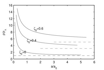
Figure 1: On the $a-\rho$ plane, we can see the differences at the different values of $\zeta_{0}$. The horizontal lines represent the values, to which the next higher curves approach. Here we assume for simplicity the parameters($\rho_{\Lambda}=1$ and $B=1$). Note that $\zeta_{0}=0$ means without viscosity.

Under this model, we put $p=p_{M}+p_{\Lambda}$, $\rho=\rho_{M}+\rho_{\Lambda}$ into Eq.(7) and get the statefinder pair as:

$$q =-\frac{3}{2}\Omega_{\Lambda}-\frac{9}{2}\frac{\zeta_{0}}{H}+\frac{1}{2}$$ (12)

$$r =\frac{27}{4}\left[3\frac{\zeta_{0}^{2}}{H^{2}}-(1-\Omega_{\Lambda})\frac{\zeta_{0}}{H}\right]+1 b$$ (12)

$$s =-\frac{3}{2}\frac{\zeta_{0}}{H}\left(1-\frac{1}{\Omega_{\Lambda}+3\frac{\zeta_{0}}{H}}\right) c$$ (12)

where the $\Omega_{\Lambda}$ is the vacuum density parameter defined by $\Omega_{\Lambda}=\rho_{\Lambda}/H^{2}$.

The expressions (12) demonstrate that the diagnostic pair $\{r,s\}$ is dependent on a single dynamically changing quantity $H$. We draw on the figure 2 the trajectories of the statefinder pair $\{r,s\}$. The point $\{0,1\}$ corresponds to the diagnostic pair $\{r,s\}$ for the $\Lambda$CDM model with no viscosity, and the curves which with the larger bulk viscosity $\zeta_{0}$ are more parabola-like represent viscous situations. The $\Lambda$CDM models that either are viscous or non-viscous are therefore differentiated by the trajectories on the $s-r$ parameters plane.

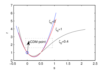
Figure 2: On the $s-r$ plane, we can see the differences with the different values of $\zeta_{0}$ . When $\zeta_{0}$ takes a smaller value, the trajectory looks not similar to a parabola. However, as $\zeta_{0}$ becomes bigger and bigger, its trajectory tends like the parabola more and more. Here we assume the parameter($\rho_{\Lambda}=1$) for simplicity. Note that $\zeta_{0}=0$(a circle) means no viscosity in this case.

III.2 Quiessence model

The Quiessence model which characterizes itself with the EoS :

$$p_{X}=w_{0}\rho_{X}$$

($w_{0}$ is constant, but asked not -1 as reason shown below, with contrast to the cosmological constant case) has been used recently to describe the dark energy behaviors. It is interesting to consider such model under the viscous situation. After assuming no interaction between two fluids $M$ and $X$, we can decompose them , that is, the $X$ and $M$ satisfy the Eqs.(4) and (5), respectively. By writing the $X$ part out independently, we have:

$$\int\frac{d\rho_{X}}{(1+w_{0})\rho_{X}-3\zeta_{0}\sqrt{\rho_{X}}}=-3\int\frac{da}{a}$$ (13)

By working the above integration out, we get

$$\rho_{X}=\left[\frac{3\zeta_{0}}{1+w_{0}}+B(1+z)^{\frac{3(1+w_{0})}{2}}\right]^{2}$$ (14)

where the redshift is denoted by $z$ with $z=a_{0}/a-1$ and $B$ is an integration constant. And the density of the non-relative matter $M$ component has possessed the following scaling relation from Eqs.(4) and (5)

$$\rho_{M}=C(1+z)^{3}$$

with a positive integration constant $C$. Then the value of the total energy density as an additive quantity can be easily composed as:

$$\rho=\left[\frac{3\zeta_{0}}{1+w_{0}}+B(1+z)^{\frac{3(1+w_{0})}{2}}\right]^{2}+C(1+z)^{3}$$ (15)

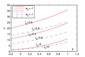
Figure 3: In the $\rho-z$ plane, we can see the differences at the different values of $\zeta_{0}$ . The viscosity makes the density bigger than that of no-viscosity cases. Here we assume the parameter($B=C=1$, and $w_{0}=-0.5or-1.5$).Note that $\zeta_{0}=0$ means that there is no viscosity.

It is a function about the scaling relation with variable $z$. Moreover, the concept of relative changing rate parameter $\varsigma$ will be used again to investigate the effects of the bulk viscosity for clarifications.

For the simplicity of discussing the parameter $\varsigma$, we first draw the relation of the Eq.(15) on the figure 3. The definition of the $\varsigma$ is modified in this case as

$$\varsigma=\frac{|\rho(z+\triangle z)-\rho(z)|}{\rho(z)}$$

where the $\triangle z$ denotes a small change of the redshift $z$. With the same analysis as in the above subsection III.1, we can still obtain the conclusion that the bulk viscosity stabilizes the evolution of the density in this model. It is worth noting that on the figure 3 the trajectories are divided into two classes corresponding to $w_{0}>-1$ and $w_{0}<-1$ respectively, and $w_{0}=-1$ is correspondence to the singularity as shown in Eq.(15) clearly. The phantom dividing phenomenonml can also appear on the statefinder pair plane as illustrated in the following discussions.

The statefinder diagnostic pair of the Quiessence model can be gotten, when we put $\rho=\rho_{M}+\rho_{X}$ and $p\simeq w_{0}\rho_{X}$ into Eq.(7). The results are:

$$q =\frac{3}{2}w_{0}\Omega_{X}-\frac{9}{2}\frac{\zeta_{0}}{H}+\frac{1}{2}$$ (16)

$$r =\frac{9}{2}(1+w_{0})w_{0}\Omega_{X}-\frac{27}{4}\frac{\zeta_{0}}{H}(w_{0}\Omega_{X}-3\frac{\zeta_{0}}{H}+1)+1 a$$ (16)

$$s =\frac{(1+2w_{0})w_{0}\Omega_{X}}{2(w_{0}\Omega_{X}-3\frac{\zeta_{0}}{H})}-\frac{3}{2}\frac{\zeta_{0}}{H}+\frac{1}{2} b$$ (16)

where the $\Omega_{X}$ denotes the dark energy density parameter defined by $\Omega_{X}=\rho_{X}/H^{2}$. Considering Eqs.(4) and (15), we can ultimately transform $q,r,s$ into such quantities depending on the redshift $z$ only.

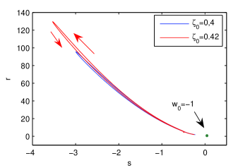
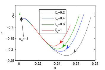
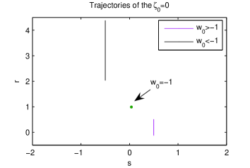
Figure 4: The above three panels are numbered from up to down as $4.1$,$4.2$ and $4.3$: $4.1$ is at the situation of $w_{0}=-1.5$; while $4.2$ is in the case of $w_{0}=-0.5$ and $4.3$ is for viscosity free $\zeta_{0}=0$ condition. Arrows represent the directions of the evolutions of statefinder diagnostic pair about time. Here we have assumed for simplicity the parameters ($B=C=1$) in the Eq.(15).

The situation of the $w_{0}=-1$ is thought as the border-case called ‘phantom divide’ (see reference WH ). The singular property of the ‘phantom divide’ can also be described by the trajectories on the statefinder pair plane in the figure 4. The corresponding relationship between the trajectories on the figure 4 and the values of the parameters are arranged in the table 1.

Table 1: Relationship between Figures and parameters

	$w_{0}>-1$	$w_{0}=-1$	$w_{0}<-1$
$\zeta_{0}>0$	curves on $4.2$	bullets on $4.1$,$4.2$	curves on $4.1$
$\zeta_{0}=0$	curves on $4.3$	bullets on $4.3$	curves on $4.3$

bullet hereafter refers to point for diagnostic pair $(s,r)=(0,1)$, i.e., corresponding to $\Lambda$CDM model
$4.1$ denotes the first panel in the figure4.
$4.2$ refers to the second panel in the figure 4.
$4.3$ represents the third panel in the figure 4.

Obviously the point of $(0,1)$ that denotes the situation of the $w_{0}=-1$ divides the trajectories into two parts, the curves of Fig.$4.1$ and the curves of Fig.$4.3$. The directions of the evolutions demonstrate that our universe is approaching the state of the $w_{0}=-1$ and then keeps itself stable there, which is consistent with results from lots of data analysis and cosmic simulations as favored to the $\Lambda$CDM model for describing later stage universe evolutions.

IV DE model with variable bulk viscosity and EoS, the entropy

In this section, we mainly discuss the viscous dark energy model which characterizes itself with the variable state parameter $w$. We here take the form of the bulk viscosity as $\zeta=\zeta_{1}\dot{a}/a$(see reference IB ; XM ) which is a particular situation of the general approaches as proposed in the reference SC . Some thermodynamic discussions, especially the entropy expression (an instructive way to obtain the entropy expression for viscous cosmology from generalized Cardy-Verlinde entropy formula can be found in Ref.bo ), are made first, and then the trajectories of the model on the statefinder diagnostic pair plane are shown. For simplicity, we only discuss the universe filled by the fluid of only one component with the following EoS SW

$$p=(\gamma-1)\rho+p_{1}$$ (17)

where the $p_{1}$ is a constant (as subscript 0 often indicating present value). For system only consisting of same mass particles, like baryons, its pressure is proportional to $nm$ where $n$ is the number density with $m$ as the mass for one particle. The $\gamma$ is the adiabatic exponent or barotropic factor, specifically, $\gamma=5/3$ in the case of extreme non-relativity, and $\gamma=4/3$ in the case of extreme relativity. As for other general cases, $\gamma$ will take complicated forms.

The $\gamma-1$ will be equivalent to the state parameter $w$ (hereafter) if the absolute value of $p_{1}$ is much smaller than that of pressure $p$. The bound on the state parameter $w$ is given out as (see reference AM ; TRC ; RO )

$$-1.38<w<-0.8$$

and thus the adiabatic exponent $\gamma$ gets its own constraint as $-0.38<\gamma<0.2$.

By directly calculations from the Eqs.(4) and (5), the scale factor is obtained as:

Provided $\widetilde{\gamma}<0$,

$$a(t)=a_{0}\left[\cosh\left(\frac{t-t_{0}}{2T_{1}}\right)+\widetilde{\gamma}\theta_{0}T_{1}\sinh\left(\frac{t-t_{0}}{2T_{1}}\right)\right]^{\frac{2}{3\widetilde{\gamma}}}$$ (18)

If $\widetilde{\gamma}>0$,

$$a(t)=a_{0}\left[\cos\left(\frac{t-t_{0}}{2T_{2}}\right)+\theta_{0}\widetilde{\gamma}T_{2}\sin\left(\frac{t-t_{0}}{2T_{2}}\right)\right]^{\frac{2}{3\widetilde{\gamma}}}$$ (19)

where $T_{1}$,and $T_{2}$ are defined by

$$T_{1}=\frac{1}{3\sqrt{-\widetilde{\gamma}p_{1}}},\quad T_{2}=\frac{1}{3\sqrt{\widetilde{\gamma}p_{1}}}$$

And where

$$\widetilde{\gamma}=\gamma-3\zeta_{1}$$

is an effective parameter for the $\gamma$, and the $\rho_{0}$, $\theta_{0}$, $t_{0}$ are the present energy density, expansion scalar, and cosmic time, respectively.

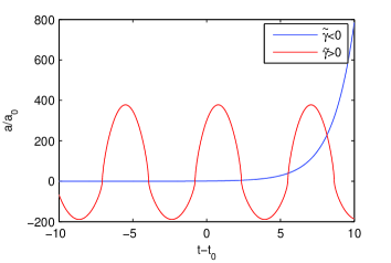
Figure 5: On the $t$-$a$ plane, the scale factor $a(t)$ at the case of $\widetilde{\gamma}>0$ shows an oscillating expansion cosmology model while the $\widetilde{\gamma}<0$ case corresponds to the late time accelerating expansion universe

Eqs.(18) and (19) are compared by the use of curves on the figure 5. As for the case of $\widetilde{\gamma}<0$, it can successfully explain the cosmic accelerating expansion in the late evolution universe. Conversely, it is impossible to do so for the case of $\widetilde{\gamma}>0$, partly because there are negative values of the scale factor $a$ which seem un-physical by the direct mathematical treatment. So it is proper for us to only consider the case $\widetilde{\gamma}<0$ in the following discussion.

The number of effective parameters from (18) is reduced to three: $T_{1}$, $\theta_{0}$, and $\widetilde{\gamma}$. For the convenience of following discussions, it is beneficial here to consider possible constraint to these parameters from the favorable fact $\dot{a}>0$ particularly in the late universe evolution. By calculating $\dot{a}$ with the use of Eq.(18), we can have

$$\dot{a}=\frac{a}{3\widetilde{\gamma}T_{1}}x^{3\widetilde{\gamma}/2}\left[\sinh(\frac{t-t_{0}}{2T_{1}})+W\cosh(\frac{t-t_{0}}{2T_{1}})\right]$$ (20)

where $W$ is defined by $W=\widetilde{\gamma}\theta_{0}T_{1}$ and $x$ is defined by $x=a_{0}/a=1+z$($z$ denotes the redshift). We have known that $a>0$, $\widetilde{\gamma}<0$, and $T_{1}>0$, and thus $\dot{a}>0$ is equivalent to

$$W<\frac{1-\exp(\frac{t-t_{0}}{T_{1}})}{1+\exp(\frac{t-t_{0}}{T_{1}})}$$ (21)

Corresponding to $t\rightarrow\infty$, as our interested later stage evolution for the observable universe, the right hand of the above inequality has possessed a limit as following

$$-1<\frac{1-\exp(\frac{t-t_{0}}{T_{1}})}{1+\exp(\frac{t-t_{0}}{T_{1}})}$$

So the constraint (21) of $W$ becomes

$$W\leq-1$$

Here we also give out, respectively, the expressions of density and expansion factor depending on the relevant variables $t$ and $z$, which will be used in our entropy expression calculations:

$$\rho(z) = \rho_{0}\left[(1+\frac{p_{1}}{\rho_{0}\widetilde{\gamma}})(1+z)^{3\widetilde{\gamma}}-\frac{p_{1}}{\rho_{0}\widetilde{\gamma}}\right]$$ (22)

$$\theta(t) = \frac{\theta_{0}}{W}\cdot\frac{\sinh(\frac{t-t_{0}}{2T_{1}})+W\cosh(\frac{t-t_{0}}{2T_{1}})}{\cosh(\frac{t-t_{0}}{2T_{1}})+W\sinh(\frac{t-t_{0}}{2T_{1}})}$$

$$\theta(z) = -\frac{\theta_{0}}{W}\cdot\sqrt{1+(W^{2}-1)(1+z)^{3\widetilde{\gamma}}}$$ (23)

For the perfect fluid models in a closed cosmic system, the cosmic media is regarded without dissipation and the entropy is a conservation quantity with $dS/dt=0$($S$ denotes the entropy of the system per unit volume). However, considering non-perfect fluid models, the entropy will change. Now we turn our attentions on the entropy of the model as introduced in this section.

The relevant general formulas to be employed (see reference IB1 ; SW1 ; AHT ) are:

$$S^{\mu}_{;\mu}=\frac{2\eta}{T}\sigma_{\mu\nu}\sigma^{\mu\nu}+\frac{\zeta}{T}\theta^{2}+\frac{1}{\kappa T^{2}}Q_{\mu}Q^{\mu}$$ (24)

where the $S^{\mu}$ is the entropy four-vector, $\eta$ the shear viscosity, $T$ the temperature, $\zeta$ the bulk viscosity, $\sigma_{\mu\nu}$ the shear tensor, $\theta$ the expansion factor, $\kappa$ the thermal conductivity and $Q_{\mu}$ as the space-like heat flux density four-vector.

The entropy four-vector $S^{\mu}$ is defined by

$$S^{\mu}=n\sigma U^{\mu}+\frac{1}{T}Q^{\mu}$$ (25)

where the $n\sigma$ is the ordinary entropy per unit volume($n$ denoted the particle number per unit volume with $\sigma$ as the entropy of one particle). The expansion tensor $\theta_{\mu\nu}$ is defined as:

$$\theta_{\mu\nu}=\frac{1}{2}(U_{\mu;\alpha}h^{\alpha}_{\nu}+U_{\nu;\alpha}h^{\alpha}_{\mu})$$

The scalar expansion factor is $\theta=\theta^{\mu}_{\mu}=U^{\mu}_{;\mu}$. The shear tensor is defined as

$$\sigma_{\mu\nu}=\theta_{\mu\nu}-\frac{1}{3}h_{\mu\nu}\theta$$

which is traceless, that is $\sigma_{\mu}^{\mu}=0$ and where the $h_{\mu\nu}$ has been defined by $h_{\mu\nu}=g_{\mu\nu}+U_{\mu}U_{\nu}$. Defining the four-acceleration of the fluid as $A_{\mu}=\dot{U}_{\mu}=U^{\nu}U_{\mu;\nu}$, the space-like heat flux density four-vector is given by

$$Q^{\mu}=-\kappa h^{\mu\nu}(T_{,\nu}+TA_{\nu})$$

In the case of thermal equilibrium, $Q^{\mu}=0$.

Under the background of FRW metric, we can have

$$\sigma_{\mu\nu}=0,\quad\theta=3H$$

Eqs.(24) and (25) yield

$$S^{\mu}_{;\mu}=\frac{\zeta_{1}}{3T}\theta^{3},\quad S^{0}=n\sigma,\quad S^{i}=0(i=1,2,3.)$$

After taking account of FRW metric, we can get the following differential equation as

$$S^{0}_{,0}+\theta S^{0}=\frac{\zeta_{1}}{3T}\theta^{3}$$ (26)

where the ‘$,0$’ denotes time derivative $d/dt$. We assume that the fluctuation of temperature is so small that it is negligible. The Eq.(26) can be transformed as

$$\frac{\theta_{0}}{2T_{1}W}\left(1-W^{2}\frac{\theta^{2}}{\theta_{0}^{2}}\right)\frac{dS^{0}}{d\theta}+\theta S^{0}=\frac{\zeta_{1}}{3T}\theta^{3}$$ (27)

Then, based on Eq.(18), we work the differential Eq.(26) out and get:

$$S^{0}=\frac{1}{1-W^{2}\theta^{2}/\theta_{0}^{2}}\left(\frac{\zeta_{1}T_{1}W}{6\theta_{0}T}\theta^{4}+Ce^{\frac{T_{1}\theta_{0}}{W}}\right)$$ (28)

where the $C$ is an integral constant. From the equation of (28), we find that when $\theta=\theta_{0}/W$, the $S^{0}$ approaches to infinity if we did not consider the values of the constant $C$. To avoid this un-physically mathematical phenomenon, we choose the value of $C$ as

$$C=-\frac{\zeta_{1}T_{1}\theta_{0}^{3}}{6TW^{3}}e^{-\frac{T_{1}\theta_{0}}{W}}$$

which will lead to such a limit that

$$\lim_{\theta\rightarrow\theta_{0}/W}S^{0}=-\frac{\zeta_{1}T_{1}\theta_{0}}{3TW}\theta^{2}$$

without the formal singularity. The expression (28) of the $S^{0}$ therefore becomes:

$$S^{0}(\theta)=-\frac{\zeta_{1}T_{1}\theta_{0}}{6W^{3}T}\cdot\frac{W^{4}\theta^{4}-\theta_{0}^{4}}{W^{2}\theta^{2}-\theta_{0}^{2}}$$ (29)

or in a more easily reading form

$$S^{0}(z)=-\frac{\zeta_{1}T_{1}\theta_{0}^{3}}{6W^{3}T}\cdot\left[2+(W^{2}-1)(1+z)^{3\widetilde{\gamma}}\right]$$ (30)

The conservation equation for the particle number is:

$$(nU^{\mu})_{;\mu}=0$$

which means that $na^{3}=constant$ in the comoving frame. Therefore the entropy for the whole observable universe in this model is

$$S(z)=(n\sigma)a^{3}=(\frac{a_{0}}{z+1})^{3}S^{0}(z)$$ (31)

By considering Eqs.(23) and (28), we can obtain

$$S(z)= -\frac{\zeta_{1}T_{1}\theta_{0}^{3}}{6W^{3}T}\cdot\left(\frac{a_{0}}{1+z}\right)^{3}\cdot$$ (32)

$$\left[2+(W^{2}-1)(1+z)^{3\widetilde{\gamma}}\right]$$

With the above expressions, we have established the relation between the entropy $S$ and the redshift $z$.

Now, we will use 157 gold data points as presented by Riess et alAGR to confront with our model and constrain parameters $W$ as well as $\widetilde{\gamma}$. In order to maximize the following likelihood function (see referencesSC ; YG ):

$$L\propto\exp[-\frac{\chi^{2}}{2}]$$ (33)

we minimize $\chi^{2}$ which here is expressed as

$$\chi^{2}=\sum_{i}\left[\frac{\mu_{obs}(z_{i})-\mu_{th}(z_{i})}{\sigma_{i}}\right]^{2}$$ (34)

where $z_{i}$, $\mu_{th}(z_{i})$, and $\sigma_{i}$ are known from Gold data. $\mu_{th}(z)$ is defined by

$$\mu_{th}(z)=5\lg\left[(1+z)\int_{0}^{z}\frac{dz^{\prime}}{h(z^{\prime})}\cdot c\right]+25$$

where $h(z)$ is the reduced Hubble parameter with $h(z)=H(z)/H_{0}=\theta(z)/\theta_{0}$. Here we have assumed curvature $k=0$ and $c$ is a constant ( also one of constrained quantities).

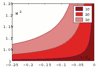
Figure 6: The likelihood contours obtained for $W^{2}$ and $\widetilde{\gamma}$ with 157 gold SNe Ia data analysis.

Through the numerical calculations, we find that the best consistent values can be taken as

$$W=-1,\quad\widetilde{\gamma}<0\quad or\quad W\leq-1,\quad\widetilde{\gamma}=0$$

Because the $\widetilde{\gamma}$ has also possessed the constraint of $\widetilde{\gamma}<0$, we can merely take $W=-1$ then. The $68.3\%$, $95.4\%$ and $99.7\%$ likelihood contours are shown on the figure 6. The next figure 7 is the comparison between experiment data and the theoretic model estimations, from which we can see that the theoretic estimations can well fit the Gold data for the smaller redshifts.

Taking $W=-1$ into Eq.(32), the expression of entropy is reduced into

$$S(z)=\frac{\zeta_{1}T_{1}\theta_{0}^{3}}{3T}\cdot\left(\frac{a_{0}}{1+z}\right)^{3}$$ (35)

in which the entropy density $S^{0}$ does not alternate, but the entropy $S$ changes as the ”volume” $a^{3}$ varies. Obviously the entropy of the Eq.(35) provides an arrow of time for cosmic evolution with the meaning that the entropy of our observable universe is always increasing.

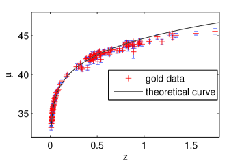
Figure 7: The comparison of experiment data and theoretical curve by fitting the 157 gold SNe Ia data

For the definition of the parameter $W$, $W=\widetilde{\gamma}\theta_{0}T_{1}$ , parameter $\widetilde{\gamma}$ when one takes $W=-1$ becomes

$$\widetilde{\gamma}=\gamma-3\zeta_{1}=-\frac{9p_{1}}{\theta_{0}^{2}}=-\frac{p_{1}}{\rho_{0}}$$

Taking the result into Eq.(22), we can get

$$\rho=\rho_{0}$$

which is a constant. Consequently, pressure $p$ also takes a constant value. Comparing these results with the well-known $\Lambda$CDM model, we may conclude that in the viscous cosmology cases, the best fitting results still favor the $\Lambda$CDM model. This point can also be reached from the view point of of statefinder diagnostic pair.

Via using the statefinder diagnostic pair $\{r,s\}$ expressions, we can obtain directly,

$$q =\frac{3}{2}V-1$$ (36)

$$r =\frac{9}{2}V(\widetilde{\gamma}-1)+1 a$$ (36)

$$s =\frac{V(\widetilde{\gamma}-1)}{V-1} b$$ (36)

where $V$ is defined by

$$V=p_{1}(\frac{1}{\rho}-\frac{1}{\rho_{0}})$$

The trajectories is show on the figure 8.

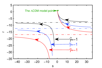
Figure 8: On the $s-r$ plane, the trajectory is a hyperbola. The present point is at $r=1$,$s=0$. The arrows indicate the cosmic parameters changing tendency, which prefers the $\Lambda$CDM model in the later cosmic evolutions.

When taking the best fitting parameter $W=-1$, we obtain $V=0$, $r=1$ and $s=0$ that is also the case of the $\Lambda$CDM model. So it confirms our previous point again that in the viscous cases, the best fitting model still returns to the conventional $\Lambda$CDM model.

V conclusions and discussions

We mainly discuss the behaviors of some viscous cosmology models on the statefinder pair plane on the purpose to mimic dark energy characters, with the hope to demonstrate that cosmic viscosity can also play the role as a possible candidate for dark energy. To this aim, we are first to give out the formulas for viscous cosmology statefinder pair expressions (7). After introducing the relative changing rate $\varsigma$, the global evolution of density is found to relax as more stable in the viscous model situations. At the same time, the trajectories of viscous universe statefinder pair on $s-r$ plane become quite different from non-viscous cases as table 2

Table 2: Relationship between models and figures

the $s-r$ plane	$\zeta=\zeta_{0}$	$\zeta=\zeta_{1}\dot{a}/a$
$\Lambda$CDM	Fig.2	$\otimes$
Quiessence	Fig.4	$\otimes$
Variable DE EoS	$\otimes$	Fig.8

$\otimes$ denotes no figures

Particularly for the Quiessence model, the singular property of the ‘phantom divide’ $w_{0}=-1$ can be clearly demonstrated on the statefinder diagnostic pair plane by the completely different trajectories to discriminate themselves. And the directions of the evolution of the trajectories on the statefinder diagnostic pair planes for the three models all point to the point of $r=1$,$s=0$ ($\Lambda$CDM model preferred), that is the universe favors simple in the later evolution stage with scale largely expanded. The $\Lambda$CDM cosmology is simply consistent with the current astrophysics observations, especially the cosmic late time accelerating expansion, but the cosmological constant has been puzzling ever since.

Additionally, we also have a try to describe the entropy of the viscous cosmology system. After adopting the EoS (17) and the bulk viscosity $\zeta=\zeta_{1}H$, we deduce out the concrete expression for the entropy. Then the 157 gold data from the supernova observation are used to constrain parameters $W$ and $\widetilde{\gamma}$, and we therefore get the most favorable parameter: $W=-1$. Further we find that the entropy of the universe is always increasing with cosmic evolution, which is consistent with the thermodynamics arrow of time.

Observational cosmology across this century has challenged our naive physics models, and with the anticipated advent of more precious data we have the chance to understand or uncover the universe mysteries by more practical modelling. Quite possibly we will get more hints to unveil the cloudy cosmological constant puzzle. In the simple constant bulk viscosity case (a proto type or a toy cosmic media model) as demonstrated in section three the vacuum energy density can be shifted by the bulk media viscosity to arrive at an effective vacuum energy density (EVED) or we may say that the constant viscosity can tune the cosmological constant in a sense if we have possessed a suitable cosmic media model. We expect more encouraging work on non-perfect fluid cosmic concord models to come soon and we believe this line of trying can contribute us new understandings to the mysterious dark side of our complicated but observable and conceivable universe.

References

- (1) D.N. Spergel et al., Astrophys. J. Suppl. 148 (2003) 175.
- (2) M. Tegmark et al., Phys. Rev. D 69 (2004) 103501.
-
(3)
A.G. Riess et al., Astron. J. 116 (1998) 1009;
S. Perlmutter et al., Astrophys. J. 517 (1999) 565. - (4) P. Coles, Nature 433, 248(2005); special section in Science 300, 1893(2003)
- (5) K. Freese and M. Lewis, Phys. Lett. B 540, 1 (2002); G.R. Dvali, G. Gabadadze, and M. Porrati, Phys. Lett. B 484, 112 (2000); G.R. Dvali and M.S. Turner. arxiv: astro-ph/0301510; A. Lue, R. Scoccimarro, and G. Starkman, Phys. Rev. D 69, 044005 (2004); S. Nojiri, S.D. Odintsov, Phys. Lett. B 599, 137 (2004; S.M. Carroll, V. Duvvuri, M. Trodden, and M.S. Turner, Phys. Rev. D 70, 043528 (2004); X.H. Meng and P. Wang, Class. Quant. Grav. 20, 4949 (2003); arxiv: hep-th/0309062; ibid, 21, 951 (2004); arxiv: astro-ph/0308284; ibid, 22, 23 (2005); arxiv: hep-th/0310038; ibid, Gen. Rel. Grav. 36, 1947; arxiv: astro-ph/0406445; ibid, Phys. Lett. B 584, 1 (2004); T. Chiba, Phys. Lett. B 575, 1, (2003); E.E. Flanagan. Phys. Rev. Lett. 92, 071101, (2004); S. Nojiri and S.D. Odintsov. Phys. Rev. D 68, 123512 (2003); D.N. Vollick. Phys. Rev. D 68, 063510, (2003).
- (6) C.W. Misner. Astrophys. J. 151, 431(1968).
-
(7)
S. Nojiri and S.D. Odintsov. Phys. Rev. D 70 (2004)
103522 and references therein.
S. Nojiri and S.D. Odintsov. arxiv: hep-th/0505215. - (8) V. Sahni. arxiv: astro-ph/0211084
- (9) Ø. Grøn. Astrophys. Space Sci. 173, 191(1990).
- (10) S. Weinberg. Phys. Rev. D 69, 023503(2004).
- (11) P. Langacher. Phy. rep. 72, 185(1981).
- (12) V. Sahni, T.D. Saini, A.A. Starobinsky and U. Alam. JETP Lett. 77 201 (2003); arxiv: astro-ph/0201498.
- (13) U. Alam, V. Sahni, T.D. Saini, A.A. Starobinsky. Mon. Not. R. Astron. Soc. 344 (2003) 1057; arxiv: astro-ph/0303009.
- (14) V. Gorini, A. Kamenshchik, U. Moschella. Phys. Rev. D 67 (2003) 063509, arxiv: astro-ph/0209395.
- (15) W. Zimdahl and D. Pavon. Gen. Relativ. Gravit. 36 (2004) 1483; arxiv: gr-qc/0311067.
- (16) S. Hannestad. arxiv: astro-ph/0509320.
-
(17)
I. Brevik and O. Gorbunova. arxiv: gr-qc/0504001;
I. Brevik, O. Gorbunova, and Y.A. Shaido. arxiv: gr-qc/0508038. -
(18)
X. Meng, J. Ren, and M. Hu. arxiv: astro-ph/0509250;
J. Ren, X. Meng. arxive:astro-ph/0511163, to appear in Phys.Lett.B. - (19) P. Gonzalez, et al, Phys. Lett. B562, 1(2003); S. Nojiri, S. Odintsov and S. Tsujikawa. Phys. Rev. D 71, 063004(2005) and references therein;
- (20) I. Brevik and S. D. Odintsov, gr-qc/0110105;
-
(21)
W. Hu. arxiv: astro-ph/0410680;
X. Meng, M. Hu, and J. Ren. arxiv:astro-ph/0510357. - (22) S. Weinberg, Gravitation and Cosmology, John Wiley & Sons, NewYork(1972).
- (23) A. Melchiorri, L. Mersini, C. J. Odman and M. Trodden. Phys. Rev. D 68 043509(2003).
- (24) T.R. Choudhary and T. Padmanabhan 2003 Preprint: astro-ph/0311622; H. Jassal, J. Bagla and T. Padmanabhan. Mon. Not. Roy. Astron. Soc. Letters 356, L11 (2005); arxiv: astro-ph/0506748.
- (25) R. Opher and A. Pelinson. arxiv: astro-ph/0505476.
- (26) I. Brevik, arxiv: gr-qc/0404095.
- (27) S. Weinberg. Astrophys. J 168, 175(1971).
- (28) A.H. Taub. Annual Rev. Fluid Mech. 10, 301(1978).
- (29) S. Capozziello, V.F. Cardone, et al., arxiv: astro-ph/0508350.
- (30) Y. Gong and Y. Zhang. arxiv:astro-ph/0502262.
- (31) A.G. Riess et al., Astrophys. J. 607 (2004) 665; arxiv: astro-ph/0402512.
- (32) I. Brevik, S. Nojiri, S.D. Odintsov, et al. Phys.Rev.D 70 (2004) 043520. arxiv: hep-th/0401073.
-
(33)
T. Padmanabhan and
S. Chitre, Phys. Lett. A120, 433 (1987);
A.D. Prisco, L. Herrera, and J. Ibanez. Phys. Rev. D 63, 023501 (2000);
L. Herrera, A.D. Prisco, and J. Ibanez. Class. Quantum Grav. 18, 1475 (2001)