Lensing Reconstruction using redshifted 21 cm Fluctuations

Abstract

We investigate the potential of second generation measurements of redshifted 21 cm radiation from before and during the epoch of reionization (EOR) to reconstruct the matter density fluctuations along the line of sight. To do so we generalize the quadratic methods developed for the Cosmic Microwave Background (CMB) to 21 cm fluctuations. We show that the three dimensional signal can be decomposed into a finite number of line of sight Fourier modes that contribute to the lensing reconstruction. Our formalism properly takes account of correlations along the line of sight and uses all the information contained in quadratic combinations of the signal. In comparison with the CMB, 21 cm fluctuations have the disadvantage of a relatively scale invariant unlensed power spectrum which suppresses the lensing effect. The smallness of the lensing effect is compensated by using information from a range of observed redshifts. We estimate the size of experiments that are needed to measure this effect. With a square kilometer of collecting area and a maximal baseline of 3 km one can achieve lensing reconstruction noise levels an order of magnitude below CMB quadratic estimator constraints at $L=1000$, and map the deflection field out to less then a tenth of a degree ($L>2000$) within a season of observations on one field. Statistical lensing power spectrum detections will be possible to sub-arcminute scales, even with the limited sky coverage that currently conceived experiments have. One should be able to improve constraints on cosmological parameters by using this method. With larger collecting areas or longer observing times, one could probe arcminute scales of the lensing potential and thus individual clusters. We address the effect that foregrounds might have on lensing reconstruction with 21 cm fluctuations.

1. Introduction

The possibility of measuring redshifted 21 cm radiation originating before and during reionization has attracted a lot or interest recently, as it promises new insights into this poorly understood epoch, when the first radiation sources turned on and eventually ionized the universe. The origin of this observable is the spin flip transition of neutral hydrogen. Fluctuations in its brightness temperature can be caused by baryonic density fluctuations, inhomogeneities in the spin temperature, and during reionization also by an inhomogeneous ionization fraction. Future observations potentially contain information about all of these fluctuation sources (Barkana & Loeb, 2005; Loeb & Zaldarriaga, 2004).

These observations could be the definitive probe of the ‘dark ages’. At present, there are several probes of the epoch of reionization. First there is the total Thomson scattering optical depth inferred from the CMB polarization on large scales points to a mean redshift of reionization, $z_{ri}=10.9^{+2.7}_{-2.3}$ (Spergel et al., 2006). This constraint is prone to large additional systematic uncertainties, as we are just beginning to understand the properties of polarized foreground emission (Page et al., 2006). The CMB offers only an integral constraint so in principle it allows for very complicated evolution scenarios of the ionized fraction, and does not contain much information as to whether the ionization process is homogeneous or not. More detailed polarization information will allow a few more numbers characterizing the reionization process to be measured (Zaldarriaga, 1997; Hu & Holder, 2003).

Quasar absorption spectra in the redshift range 5.5-6.5 indicate a fast evolution of the ionized fraction while $x_{H}>10^{-3}$ (see e.g. Fan et al. 2005). They carry a Gunn-Peterson trough (Gunn & Peterson, 1965), suggesting incomplete ionization of the intergalactic medium (IGM) along the sight line. The sizes of the HII regions directly surrounding the quasars can be used to infer a tighter constraint on the minimal neutral fraction, $x_{H}>0.1$ since the IGM has to be somewhat neutral otherwise the regions would be larger (Wyithe et al., 2005).

The redshifted 21 cm line is outstanding in comparison to CMB and quasar observation studies because it should be sensitive to order unity changes in the neutral fraction $x_{H}$, hence probing the middle stages of reionization. It will also provide well-localized measurements along the line of sight, and it will not require the background of bright sources which might be rare at high redshifts.

Although 21 cm measurements offer the possibility to constrain the state of the IGM during the end phases of reionization, due to the confounding effects of their unknown astrophysics it might be difficult to compete with the constraints on cosmological parameters (McQuinn et al., 2005) coming from microwave background experiments such as the Planck satellite , the E and B experiment (EBEX) (Oxley et al., 2004). the Atacama Cosmology Telescope (ACT) (Kosowsky, 2003), or the South Pole Telescope (SPT) (Ruhl et al., 2004)).

In this paper we will explore the information contained in the intrinsically three dimensional 21 cm measurement about the intervening mass distribution at lower redshifts through the lensing effect. We generalize the quadratic estimator technique developed by Hu (2001b) to a three dimensional observable. Our formalism uses all the information in both shear and convergence and properly takes account of correlations along the line of sight. Before the ionized fraction of the IGM becomes substantial, the 21 cm emission against the CMB is a near Gaussian random field. In this regime, which is the focus of the present article, the quadratic estimator should be close to optimal Hirata & Seljak (2002).

We will look at 21 cm fluctuations at their lowest possible redshift range, $z=6-12$, where the second generation of experiments might be able to measure at high signal-to-noise. Using our formalism we can also estimate information losses due to foreground contamination, once these are described by some model. We also explore the possibility to constrain the dark energy density with lensing of the 21 cm background. Another application would be to measure nonlinearities in the density field. We compare our results to the potential of a future high precision observation of the CMB. The CMB damping tail is an advantage for lensing reconstruction since reconstruction errors decrease with increasing slope, but at the same time it leads to a small scale limitation for CMB reconstruction, as the signal quickly falls below the noise.

Lensing reconstruction using the redshifted 21 cm radiation in absorption against the CMB has been investigated by Cooray (2004), in particular also the possibility to get a handle on gravity waves from inflation by gravitational lensing cleaning of B mode polarization (lensing converts E to B modes of the polarization and acts as a contaminant to the primordial signal) (Sigurdson & Cooray, 2005). Their work describes two types of observations, which employ a 20/200 times larger total collecting area than we will assume here (and five times longer observation time) to observe angular fluctuations $L_{max}=5000-10^{5}$ in the 21 cm field. The problem is that the prospect, beating the CMB level for B mode lensing cleaning, relies on measuring the 21 cm power spectrum at very high redshifts (they use $z_{\rm source}=30$), at which the galactic synchrotron contamination is a factor $\simeq 20$ larger than for example at redshift $8$. The reason such high redshift observations are needed to compete with likelihood based lensing estimation is that there is a partial delensing bias when comparing lenses out to different redshifts and $z_{s}=30$ turns out to be close enough to the last scattering surface of the CMB, where gravity waves are expected to create the B mode fluctuations. These authors furthermore make the approximation of treating their slices through the 21 cm measurement cube as uncorrelated, which is not warranted.

Pen (2004) suggested measuring the effective convergence from the effect it has on the real space variance map of 21 cm fluctuations. The author also presented rough sensitivity estimates for LOFAR, PAST, and SKA. We improve on this by using all the available information in convergence and shear in an optimal way and use more realistic errors.

In section 2 we will review the theory of the redshifted 21 cm signal in different regimes, which leads to the distinction of a neutral phase where the brightness temperature fully traces the baryonic fluctuations, as well as a patchy phase, which can be modeled separately.

In section 3 we review the quadratic estimator technique for lensing reconstruction following Hu (2001a). Then we naturally expand the formalism to the extraction of weak lensing from an intrinsically three dimensional signal. The decomposition of the line of sight component of the signal into modes leads to a hierarchy of independent lensing backgrounds that can be probed with varying precision. Although our concentration lies on applying the quadratic estimator to the epoch immediately before substantial ionization occurs, we scrutinize its applicability to the patchy regime by using an analytic model for the morphology of HII regions.

In section 4 we put our investigation in the context of experiments, estimating the potential redshift range in which they will observe. Because signal and noise are evolving with redshift, we break down the volume of the observation in smaller boxes along the line of sight. We calculate estimates for the lensing reconstruction future 21 cm experiments might be able to achieve.

We present results based on current rough specifications of the Square Kilometer Array (SKA) in Section 5 and compare them to the possibility of constraining the matter power spectrum with the CMB temperature and polarization. The 21 cm approach turns out to have no angular scale limitation for constraining the convergence. We address limitations due to the galactic foreground and show how these can be incorporated into our formalism in a straightforward manner. We conclude with an outlook and discussion in section 6.

A $\Lambda$CDM cosmology is assumed throughout all calculations, with parameters $\Omega_{m}=0.3$, $\Omega_{\Lambda}=0.7$, $\Omega_{b}=0.04$, $H_{0}=100{\rm hkm/sec/Mpc}$ (with h=0.7), and a scale-invariant primordial power spectrum with $n=1$ normalized to $\sigma_{8}=0.9$ at the present day.

2. Theory of the redshifted 21 cm signal

The shape of the 21 cm fluctuations is easy to predict in the absence of radiative sources or in a rather homogeneous radiation background. Then it is simply proportional to the matter power spectrum which we know based on measurements of the CMB, galaxy surveys, etc. In the presence of fluctuations in the ionization fraction, the observable is more difficult to quantify, due to our lack of knowledge about the spectrum and efficiency of first sources, and the difficulty of modelling feedback processes. Some progress has been made using radiative transfer codes (Sokasian et al., 2003) on up to 20 ${\rm Mpc/h}$ scales, but because of the large size of the HII regions that simple analytic considerations suggest (Wyithe & Loeb 2004; Furlanetto et al. 2004a) it may be helpful for understanding the large scale morphology of HII bubbles to also use analytic models, such as the one based on extended Press-Schechter theory by Furlanetto et al. (2004b).

The optical depth of a region of the IGM in the hyperfine transition is (Field, 1959)

$$\tau = \frac{3c^{3}\hbar A_{10}\,n_{\rm HI}}{16k\nu_{0}^{2}\,T_{S}\,H(z)}$$ (1)

$$\approx 8.6\times 10^{-3}(1+\delta_{s})x_{H}\left[\frac{T_{\rm CMB}(z)}{T_{S}}\right]\left(\frac{\Omega_{b}h^{2}}{0.02}\right)$$

$$\times\left[\left(\frac{0.15}{\Omega_{m}h^{2}}\right)\,\left(\frac{1+z}{10}\right)\right]^{1/2}.$$

Here $\nu_{0}=1420.4\,{\rm MHz}$ is the rest-frame hyperfine transition frequency, $A_{10}=2.85\times 10^{-15}s^{-1}$ is the spontaneous emission coefficient for the transition, $T_{S}$ is the spin temperature of the IGM (i.e., the excitation temperature of the hyperfine transition), $T_{\rm CMB}=2.73(1+z){\rm K}$ is the CMB temperature at redshift $z$, and $n_{\rm HI}$ is the local neutral hydrogen density. In the second equality, we have assumed sufficiently high redshifts such that $H(z)\approx H_{0}\Omega_{m}^{1/2}(1+z)^{3/2}$, which is well-satisfied in the era we study, $z>6$. The local baryon overdensity is $1+\delta_{s}=\bar{\rho}/\rho$ and $x_{H}$ is the neutral fraction. Here the index in the overdensity emphasizes that we are measuring quantities in redshift space. The radiative transfer equation in the Rayleigh-Jeans limit tells us that the brightness temperature of a patch of the sky (in its rest frame) is $T_{b}=T_{\rm CMB}e^{-\tau}+T_{S}(1-e^{-\tau})$. Then the observed brightness temperature increment between this patch, at an observed frequency $\nu$ corresponding to a redshift $1+z=\nu_{0}/\nu$, and the CMB is

$$\delta T(\nu) \approx \frac{T_{S}-T_{\rm CMB}}{1+z}\,\tau$$

$$\approx\, 26\,(1+\delta_{s})x_{H}\left(\frac{T_{S}-T_{\rm CMB}}{T_{S}}\right)\left(\frac{\Omega_{b}h^{2}}{0.022}\right)$$ (2)

$$\times\left[\left(\frac{0.15}{\Omega_{m}h^{2}}\right)\,\left(\frac{1+z}{10}\right)\right]^{1/2}{\rm mK}.$$

So if the excitation temperature $T_{s}$ in a region differs from that of the CMB, the region will appear in emission (if $T_{s}>T_{\rm CMB}$) or absorption (if $T_{s}<T_{\rm CMB}$) against the CMB.

Ciardi & Madau (2003) argue that the intensity of the Ly$\alpha$ background is large enough at all relevant redshifts, so that Ly$\alpha$ pumping (the Wouthuysen-Field effect (Wouthuysen, 1952; Field, 1958), in combination with the fact that the color temperature is in thermodynamic equilibrium with the gas kinetic temperature in an optically thick medium, effectively couples the spin temperature to the kinetic temperature of the gas. Between the CMB last scattering at redshift $z\approx 1000$ and $z\approx 140$, Thomson scattering of the CMB photons effectively leads to $T_{\rm CMB}\simeq T_{K}$, but the gas decouples at $z\simeq 140$ and cools adiabatically until significant structure begins to form. For the regime we are interested in, $z<15$, it is likely that the first supernovae and/or accreting black holes produced enough high energy photons to heat the IGM Madau et al. (1996). In this case it can be assumed that a relatively homogeneous X-ray background leads to $T_{S}\approx T_{K}\gg T_{\rm CMB}$ (e.g. Ciardi & Madau 2003; Madau et al. 1996) so that the temperature factor in Equation 2 becomes simply unity. In this picture inhomogeneous effects on the brightness temperature due to shock heating along sheets and filaments are a minor contribution.

The 21 cm power spectrum is measured in redshift space, hence it is is related to the actual density contrast power spectrum through

$$P_{s}({\bf k})=P_{\delta}(k)[1+f\mu_{k}^{2}]^{2}$$ (3)

where f is the linear growth rate, $f\equiv\frac{a}{D_{1}}\frac{dD_{1}}{da}$. The cosine of the angle between the line of sight $\hat{z}$ and the wavevector ${\bf k}$ is denoted $\mu_{k}$.

Here we will assume that in the regime of interest $f\simeq 1$, hence we obtain with $T_{s}\gg T_{\rm CMB}$ that the power spectrum of the 21 cm brightness temperature fluctuation in the neutral regime is given by

$$P_{\Delta T_{b}}(k)\simeq(26{\rm mK})^{2}\frac{1+z}{10}(1+\mu_{k}^{2})^{2}P_{\delta}(k)$$ (4)

In this paper, we shall be mainly concerned with quadratic estimator lensing reconstruction during this highly neutral regime. The extension to a patchy epoch is complicated by the presence of a connected four-point function contribution to the source field. On the level of the power spectrum this contribution acts as a sample variance term, correlating different k-modes. In the following paragraph we shall discuss a semi-analytic model that can be used to describe the patchy regime. In the analysis section we will briefly estimate the application of our estimator to this regime.

The fluctuating 21 cm brightness temperature simply traces the matter fluctuations until the time when the IGM starts getting significantly ionized. Current radiative transfer codes do not allow dynamical ranges large enough to simulate the reionization morphology on scales above $20{\rm Mpc/h}$. To model the patchy regime we implement the analytic model suggested by Furlanetto et al. (2004b) into the three dimensional signal Gaussian random fields of sidelength $1000{\rm Mpc/h}$ comoving (compare Zahn et al. 2005) with a resolution of $512^{3}$. In the extended Press-Schechter formalism the condition for a region to be ionized, $\zeta f_{\rm coll.}>1$ leads to a condition on the mean overdensity within a region of mass m (Furlanetto et al., 2004b),

$$\delta_{m}\geq\delta_{x}(m,z)\equiv\delta_{c}(z)-\sqrt{2}K(\zeta)[\sigma^{2}_{\rm min}-\sigma^{2}(m)]^{1/2}$$ (5)

where $K(\zeta)\equiv{\rm erf}^{-1}(1-\zeta^{-1})$, $\zeta$ is the ionization efficiency factor, $\sigma^{2}(m)$ is the variance of density fluctuations on the scale $m$, and $\delta_{c}(z)=1.686/D(a)$ is the critical density for collapse scaled to today, with $D(z)$ the scale factor. $\sigma^{2}_{\rm min}$ is the variance on the scale of fluctuations on the scale $m_{\rm min}$ the mass for which $T=10^{4}K$ at virialization.

Figure 1 shows the angular power spectrum of 21 cm fluctuations at redshift 8 for different values of the efficiency and therefore ionization fraction. We see that up to an ionization fraction of $x_{i}=0.7$ the signal on small scales decreases (structures below the bubble scale are washed out) while the ionized regions lead to a bump in the power spectrum on scales $k\simeq 0.2{\rm Mpc/h}^{-1}$ which corresponds to an angular multipole at the relevant redshifts of approximately $l=1000$. At even higher ionized fractions, the entire patchy power spectrum lies below the neutral case, so it becomes more difficult to observe the fluctuations and hence to use them for lensing reconstruction.

Figure 1.— Power spectrum of the 21 cm signal at various stages during reionization. The thick solid line shows the expected noise for SKA for a flat configuration of antennas inside a circle of diameter $2$ km. When the ionization fraction rises during the expansion of HII spheres, first the overall signal decays, then bubbles cluster quickly to form large ionized regions tens of ${\rm Mpc/h}$ across. This can lead to a significant increase in the signal on scales that the first imaging 21 cm experiments should be sensitive to. On the smallest scales the signal is decreased, making usage of $21$ cm fluctuations for lensing reconstruction somewhat more difficult.

In any event it seems from Figure 1 that a significant part of the patchy regime can be used for the lensing reconstruction, in part because the boosted amplitude on scales $l\simeq 100-1000$ might aid somewhat in this effort. We will evaluate these estimates more carefully in Section 5. Our choice of ionization efficiency lets reionization begin at redshifts around 8 and evolves rather slowly, due to photon consumption by clumps in the IGM. It evolves through $x_{i}\simeq 50\%$ at redshift 7 to complete at redshift 6.

We will assume a bandwidth of $B=5{\rm MHz}$ for calculating the power spectrum at various redshifts. This corresponds to a redshift interval $\Delta z=0.286$. During the neutral phase the density fluctuations evolve slowly, however the sensitivity of the experiments change rapidly with observation frequency. Because the comoving length scale is given in terms of bandwidth through

$$\mathcal{L}\approx 1.2\left(\frac{B}{0.1{\rm MHz}}\right)\left(\frac{1+z}{10}\right)^{1/2}\left(\frac{\Omega_{m}h^{2}}{0.15}\right)^{-1/2}{\rm Mpc/h},$$ (6)

our window in frequency space corresponds to a depth of 50 ${\rm Mpc/h}$ at z=6 and to 70 ${\rm Mpc/h}$ at z=12. When the first extended HII regions start forming, the power spectrum evolves more rapidly, however reionization still only lapses over a comoving length of about 300 Mpc/h, in comparison to which our window is small.

We will generate 21 cm brightness temperature power spectra following Formula 4 using linear power spectra that contain the acoustic oscillation amplitude generated from CMBFAST transfer functions (Seljak & Zaldarriaga, 1996). The baryonic wiggles included in the code might aid somewhat in our reconstruction endeavour, for reasons given in the next section. We use the same transfer functions to implement the signal in three dimensional Gaussian random fields and model the patchy phase.

3. Weak Lensing Reconstruction

3.1. Quadratic Estimator, General Consideration

Lensing by large scale structure happens whenever there is a fluctuating background field. At position ${\bf\hat{n}}$ we observe the field

$$T({\bf\hat{n}})=\tilde{T}({\bf\hat{n}}+\nabla\phi)$$ (7)

where $\tilde{T}$ denotes the unlensed field, $\delta\theta=\nabla\phi$ is the displacement vector while $\phi$ is the projected potential. Here and in what follows, boldface quantities denote vectors. The projected potential is given in terms of the gravitational potential $\psi({\bf x},D)$, where ${\bf x}$ is position and D is used as a time variable, as

$$\phi({\bf\hat{n}})=-2\int d\mathcal{D}\frac{\mathcal{D}_{A}(\mathcal{D}_{s}-\mathcal{D})}{\mathcal{D}\mathcal{D}_{s}}\psi(D{\bf\hat{n}},D)\,.$$ (8)

So the power spectrum of the displacements is $C_{L}^{\delta\theta\delta\theta}=L(L+1)C_{L}^{\phi\phi}$.

An estimator $D({\bf\hat{n}})$ for the lensing displacement field information contained in the temperature field should contain an even number of temperature terms since the expectation value for odd powers would vanish. It must also satisfy the condition

$$\langle D({\bf\hat{n}})\rangle=\delta\theta({\bf\hat{n}})$$ (9)

when averaged over many realizations of the background radiation field, that is for example the CMB or 21 cm radiation.

Hu (2001a) showed that the divergence of the temperature-weighted gradient of the map achieves maximal signal-to-noise among quadratic statistics. In Fourier space this quadratic estimator takes the form (Hu & Okamoto, 2002)

$$D_{\rm est.}({\bf L})=A(L)\int\frac{d^{2}l}{(2\pi)^{2}}F({\bf l},{\bf L}-{\bf l})T({\bf l})T({\bf L}-{\bf l})$$ (10)

The Filter $F({\bf l},{\bf L}-{\bf l})$ is obtained by minimizing the variance of $D_{\rm est.}$ under the normalization condition for $D({\bf L})$

$$F({\bf l},{\bf L}-{\bf l})=\frac{[C_{l}{\bf L}\cdot{\bf l}+C_{L-l}{\bf L}\cdot({\bf L}-{\bf l})]}{2{\tilde{\rm C}^{\rm tot}}_{l}{\tilde{\rm C}^{\rm tot}}_{L-l}}$$ (11)

and the normalization is

$$A(L)=L\left[\int\frac{d^{2}l}{(2\pi)^{2}}\frac{[C_{l}L\cdot l+C_{L-l}L\cdot(L-l)]}{2\,{\tilde{\rm C}^{\rm tot}}_{l}{\tilde{\rm C}^{\rm tot}}_{L-l}}\right]^{-1}$$ (12)

Here ${\tilde{\rm C}^{\rm tot}}_{l}$ is the sum of the lensed angular power spectrum of 21 cm fluctuations ${\tilde{\rm C}}_{l}$ and the noise power spectrum which we will give in the next section, $C_{l}^{N}$. As shown by Mandel & Zaldarriaga (2005), the effect of lensing on the angular 21 cm power spectrum for an individual plane is small, so one can use the unlensed power spectrum in place of it. The high-pass shape of the quadratic estimator gives it a property all reconstruction methods share, that they extract most information from the smallest scales resolved by some experiment. We emphasize that the estimator is unbiased by construction (Equation 9), independent of Gaussianity of the source field.

With the definition of the lensing reconstruction noise power spectrum $N_{L}$

$$\langle D^{*}({\bf L})D({\bf L}^{\prime})\rangle=(2\pi)^{2}\delta({\bf L}-{\bf L}^{\prime})(C_{L}^{DD}+N_{L})$$ (13)

evaluation of the variance of Equation 10, $\langle||D({\bf L})||^{2}\rangle=(2\pi)^{2}\delta^{D}(0)N_{L}^{D}$ gives

$$N_{L}(L) = L^{2}\left[\int\frac{d^{2}l}{(2\pi)^{2}}\frac{[C_{l}\;{\bf L}\cdot{\bf l}+C_{L-l}\;{\bf L}\cdot({\bf L}-{\bf l})]^{2}}{2\,{\tilde{\rm C}^{\rm tot}}_{l}\,{\tilde{\rm C}^{\rm tot}}_{L-l}}\right]^{-1}$$ (14)

$$= A(L)L$$ (15)

Roughly, when $L^{2}C_{L}^{\phi\phi}=N_{L}$, then structures down to the angular size $2\pi/L$ in the lensing field can be reconstructed.

We illustrate the different power spectrum characteristics of CMB and 21 cm in Figure 2.

Figure 2.— CMB temperature and E polarization power spectrum and noise levels of our example experiments: Planck and a futuristic polarized satellite mission (see text for specifications). The 21 cm power spectrum has been rescaled to fit into the same plot. The CMB exhibits more pronounced peaks and a sharp decay on scales $l\simeq 2500$ above which the Sunyaev-Zel’dovich effects become important.

We can investigate qualitatively which properties of the power spectrum set the effectiveness of this estimator by looking at the limit ${\bf L}\rightarrow 0$ (on scales where the noise is small and the lensed power is not systematically larger than the unlensed, ${\tilde{\rm C}^{\rm tot}}_{l}={\tilde{\rm C}}_{l}+{\rm C}_{l}^{N}\simeq{\tilde{\rm C}}_{l}\simeq{\rm C}_{l}$)

$$(L^{2}N_{L})^{-1} = \frac{1}{L^{4}}\int\frac{d^{2}l}{(2\pi)^{2}}\frac{[{\bf L}\cdot{\bf l}C_{l}+{\bf L}\cdot({\bf L}-{\bf l})C_{L-l}]^{2}}{2{\tilde{\rm C}^{\rm tot}}_{l}{\tilde{\rm C}^{\rm tot}}_{L-l}}$$

$$\simeq \int\frac{dl}{l}\frac{l^{2}}{2\pi}(\frac{1}{2}+\frac{1}{2}\alpha+\frac{3}{16}\alpha^{2})+$$

$$+L^{2}\int\frac{d^{2}l}{(2\pi)^{2}}\frac{1}{l^{2}}g(\alpha,\beta,\gamma)$$

where

$$g(\alpha,\beta,\gamma)=\frac{3(5\beta+8\gamma)+\alpha(\alpha(2+\alpha)(14+5\alpha+20\gamma))}{384}\,,$$ (17)

and $\alpha\equiv\frac{dlnC_{l}}{dlnl}$, $\beta=\frac{d^{2}{\rm ln}C_{l}}{d{\rm ln}l^{2}}$, $\gamma=\frac{d^{3}{\rm ln}C_{l}}{d{\rm ln}l^{3}}$. The integrand of the first order term has its minimum close to a value $\alpha=-2$, in other words when $l^{2}C_{l}$ has no slope. This implies that the CMB with its exponential decay on small scales will have a lower value of $N_{L}$ if those scales are resolved. Integrating Equation LABEL:eq:lowlest to the maximum multipole $l_{\rm max}$ at which $C_{l}^{S}>C_{l}^{N}$ leads to

$$(L^{2}N_{L})^{-1} \simeq \frac{1}{2\pi}(\frac{1}{2}+\frac{1}{2}\alpha+\frac{3}{16}\alpha^{2})\frac{l_{\rm max}^{2}}{2}$$

$$+\frac{L^{2}}{2\pi}g(\alpha,\beta,\gamma){\rm ln}(l_{\rm max}/l_{\rm min})\,,$$

where $l_{\rm min}$ is the lower bound of the integration. The second term will lead to departures from a constant value of $(L^{2}N_{L})$. The scale at which both terms are comparable is

$$L_{\rm comp.}\simeq\frac{l_{\rm max}}{{\rm ln}(l_{\rm max}/l_{\rm min})^{1/2}}\sqrt{\frac{1+\frac{1}{2}\alpha+\frac{3}{16}\alpha^{2}}{g(\alpha,\beta,\gamma)}}\,.$$ (20)

Evaluation of this expression shows that for a sloped power spectrum $l^{2}C_{l}$, such as that of the CMB, $L_{\rm comp.}$ is lower than for a spectrum that is nearly constant, such as that of 21 cm fluctuations. The second order term contributes strongly when the slope is large. If the measured power spectrum has a small slope, as is the case with 21 cm fluctuations, $L^{2}N_{L}$ can be expected to be nearly constant to the scale $l_{\rm max}$ where noise becomes important.

In the following section we will generalize the quadratic estimator to a three dimensional observable that is used to reconstruct the lensing field. The final estimator is then simply the sum of estimators of k modes along the line of sight. This allows one to improve the constraints above those by the CMB especially on small scales by summing over sufficiently many lensing backgrounds.

For our analysis in Section 4 we will compute the angular power spectrum of the deflection angle as the integral over line of sight

$$C^{\delta\theta\delta\theta}_{L}=\frac{9H_{0}^{4}\Omega_{0}^{2}}{L(L+1)c^{2}}\int_{0}^{D_{s}} dD_{l}\left(\frac{D_{ls}}{D_{s}\,a(D_{l})}\right)^{2}\times$$ (21)

$$\times P_{\delta}(k=\frac{L}{D_{l}},D_{l})$$

over the power spectrum of mass fluctuations. $D_{x}$ denote angular diameter distances with $x=l,s$ for lens and source.

We use the halo model fitting function to numerical simulations of Smith et al. (2003) to generate nonlinear $\Lambda$ CDM power spectra as input for the deflection angle integral.

3.2. Extension to a three dimensional signal

Different from the CMB, in the case of 21 cm brightness fluctuations we will be able to use multiple redshift information to constrain the intervening matter power spectrum. One could imagine applying this estimator to succesive planes prependicular to the line of sight. However the different planes would be correlated and there is no straightforward criterion to take this correlation into account in establishing the final estimator, since it would depend on redshift, source properties, and during reionization on the mean bubble size and distribution. Instead we will use the knowledge of the three-dimensional information in a different way, dividing the temperature fluctuations in Fourier space in fluctuations ${\bf k}_{\bot}$ perpendicular to the line of sight, and a component $k_{\|}$ in the frequency direction.

We devide a volume on the sky to be probed by a given 21 cm survey into a solid angle $d\Omega$ and a radial coordinate $z$. Components of wavevectors along the line of sight are described by $k_{\|}$ and those perpendicular to the line of sight are given by the vector ${\bf k}_{\bot}$, which is related to the multipole numbers of the spherical harmonic decomposition on the sky as ${\bf l}={\bf k}_{\bot}\mathcal{D}$, where $\mathcal{D}$ is the angular diameter distance to the volume element we are probing.

Suppose we want to measure a field $I({\bf r})$ with power spectrum $P({\bf k})=P({\bf k}_{\bot},k_{\|})$. Converting $k_{\bot}$ to angular multipole

$$I({\bf r}) = \int\frac{d^{3}k}{(2\pi)^{3}}I({\bf k})e^{i{\bf k}\cdot{\bf r}}$$

$$= \int\frac{d^{2}l}{(2\pi)^{2}}\int\frac{dk_{\|}}{2\pi}\frac{I({\bf k}_{\bot},k_{\|})}{\mathcal{D}^{2}}e^{i({\bf l}\cdot\theta+k_{\|}z)}$$

with $\tilde{I}({\bf l},k_{\|})=\frac{I({\bf k}_{\bot},k_{\|})}{D^{2}}$ we have

$$\langle\tilde{I}({\bf l},k_{\|})\tilde{I}({\bf l}^{\prime},k_{\|}^{\prime})\rangle = \delta^{D}({\bf k}-{\bf k}^{\prime})(2\pi)^{3}\frac{P({\bf k}_{\bot},k_{\|})}{\mathcal{D}^{4}}$$ (23)

$$= (2\pi)^{2}\delta^{D}({\bf l}-{\bf l}^{\prime})(2\pi)\delta^{D}(k_{\|}-k_{\|}^{\prime})\times$$

$$\times\frac{P({\bf k}_{\bot},k_{\|})}{\mathcal{D}^{2}}$$

where in the second step a factor of $\mathcal{D}^{2}$ got absorbed into $\delta^{D}({\bf l}-{\bf l}^{\prime})$ because of ${\bf l}={\bf k}_{\bot}\mathcal{D}$.

Let us discretize the z direction of a real space observed volume with radial length $\mathcal{L}$,

$$k_{\|}=j\frac{2\pi}{\mathcal{L}},\quad\delta^{D}(k_{\|}-k_{\|}^{\prime})=\delta_{j_{1}j_{2}}(\frac{\mathcal{L}}{2\pi})$$ (24)

so that

$$I({\bf r})=\int\frac{d^{2}l}{(2\pi)^{2}}\sum_{j}\left(\frac{I({\bf k}_{\bot},k_{\|})}{\mathcal{D}^{2}\mathcal{L}}\right)e^{i{\bf k}\cdot{\bf r}}$$ (25)

It makes sense to define

$$\hat{I}\equiv\frac{I({\bf k}_{\bot},k_{\|})}{\mathcal{D}^{2}\mathcal{L}}$$ (26)

so that on the sphere we have

$$\langle\hat{I}_{j_{1}}({\bf l}_{1})\hat{I}^{*}_{j_{2}}({\bf l}_{2})\rangle=(2\pi^{2})\delta^{D}({\bf l}_{1}-{\bf l}_{2})\delta_{j_{1}j_{2}}\left(\frac{P(k,\mu_{k})}{\mathcal{D}^{2}\mathcal{L}}\right)$$ (27)

where $\mu_{k}$ is the cosine between the wave vector and the line of sight.

We have for the angular power spectrum for separate values of j that (including redshift space distortions)

$$C_{l,j}\equiv(1+\mu_{k}^{2})^{2}\frac{P(\sqrt{(l/\mathcal{D})^{2}+(j\,2\pi/\mathcal{L})^{2}})}{\mathcal{D}^{2}\mathcal{L}}\,,$$ (28)

where P now represents the spherically averaged power spectrum. We have also introduced the notation $C_{l,j}$, denoting the power in a mode with angular component l and radial component $k_{j}=j\,2\pi/\mathcal{L}$.

We show in the Appendix that because modes with different j can be considered independent, the best estimator can be obtained by combining the individual estimators for separate j’s without mixing them (in the sense of making quadratic combinations of them). As long as the IGM is not substantially ionized, the assumption of Gaussianity is justified at the redshifts of interest, $z\simeq 6-12$, where non linearites in the gravitational clustering are small on observed scales of several Mpc/h. We find the three dimensional lensing reconstruction noise defined by

$$\langle D({\bf L})D^{*}({\bf L}^{\prime})\rangle=(2\pi)^{2}\delta({\bf L}-{\bf L}^{\prime})N_{L}^{D}$$ (29)

to be (Equation A21 of the Appendix, where e.g. ${\rm C}_{l}\rightarrow{\rm P}_{l}$)

$$N_{L}^{D} = \frac{1}{\sum_{k}\frac{1}{L^{2}}\int\frac{d^{2}l}{(2\pi)^{2}}\frac{[{\rm C}_{l,k}{\bf L}\cdot{\bf l}+{\rm C}_{L-l,k}{\bf L}\cdot({\bf L}-{\bf l})]^{2}}{2{\tilde{\rm C}^{\rm tot}}_{l,k}{\tilde{\rm C}^{\rm tot}}_{L-l,k}}}$$ (30)

$$= \frac{1}{\sum_{k}N_{L,k}^{-1}}$$ (31)

where in the last line we have just substituted the standard expression, Equation 15. Note that analogous to the CMB case, ${\tilde{\rm C}^{\rm tot}}_{l}={\tilde{\rm C}}_{l}+C_{l}^{N}$, where $C_{l}^{N}$ is the noise power spectrum, and ${\tilde{\rm C}}_{l}\simeq{\rm C}_{l}$ in the case of 21 cm fluctuations.

If there is a connected four point function contribution during the epoch of extended HII regions, this will add a term to the variance of the estimator. This will change the weightings $A_{L}$ as well, and make the estimator suboptimal. We will not try to come up with an estimator that is fully compatible with the non Gaussian signal due to patchy reionization. Instead, in the next section we will conservatively estimate that sensitivities get worse by a factor $\frac{1}{\sqrt{x_{H}}}$, where $x_{H}$ is the ionized fraction. In other words, we will effectively be treating the patchy regions as part of the source field which can be masked.

Let us examine the contribution of the components $C_{l,j}$ to the total noise in the estimation of the deflection field. From Equation 28 we see that with higher values of the component $k\|$, higher values of the three dimensional power spectrum $P(k)$ will translate into each $C_{l}$ value. But $P(k)$ is monotonically falling on all scales of interest (foregrounds can be expected to contaminate constraints below ${\rm k}<10^{-2}{\rm h/Mpc}$, the scale of the horizon at matter radiation equality and the turnover of the power spectrum), so that effectively the angular power spectrum amplitude will drop with $j$ towards the noise level. We show this in Figure 3 for our bandwidth choice of $5{\rm MHz}$. Notice that on the smallest resolved scales, $l\simeq 2000-5000$ the signal increases slightly as we go from the fundamental $k_{\|}=0$ to the next higher modes in our line-of-sight decomposition. This is because the radial component of the power spectrum is increased due to redshift space distortions. Because the smallest resolved angular scales contribute most to the lensing reconstruction, in case of the first few modes in the $k_{\|}$ decomposition this increase overcompensates for the general decay of $C_{l,j}$ on the smallest scales. However overall for each rectangular data field of a given bandwidth we will only be able to sample a limited number of modes $k_{\|}$ with signal-to-noise greater than one, this number being proportional to the frequency depth/bandwidth of the field.

Figure 3.— The dotted lines show the angular power spectrum for different $k_{\|,j}=j\,2\,\pi/L$, labeled by $j$. Going to higher values of $j$, the signal decays quickly below S/N=1 and only the first 15 or so modes contribute to the final lensing estimator. This number depends of course on the thickness of the redshift interval probed (in this case $B=5{\rm MHz}$, corresponding to $\Delta z=0.286$ at $z=8$). The thick and thin solid curves are for a flat and a cored antenna configuration of SKA (see the text).

The 21 cm power spectrum and, as we will see in the next section, the noise of the experiment depend on redshift, so we calculate them for volume elements corresponding to the above choice a $5{\rm MHz}$ bandwidth. Beginning at the end of reionization, each volume element contributes to reducing the reconstruction noise while we go along, until the signal-to-noise of the experiment at high redshift becomes negligible. We should wonder whether long wavelength modes overlapping neighbouring volumes lead to an underestimation of the final lensing noise, as we are treating each volume element as uncorrelated. We made a simple test by comparing the $N_{L}$ of a pair of neighbouring volumes to the sum of $N_{L}$’s of each element. With our choise of a $5{\rm MHz}$ bandwidth we found no excess information $>1\%$ in the sum of the seperated field’s $N_{L}$’s, meaning that we can safely neglect those correlations. A multiplicity of those volumes can thus be used to reconstruct each lens just by summing over them.

4. Antenna Configuration, Sensitivity Calculation

We have found out in the previous section that in order to measure the lensing signal with redshifted 21 cm fluctuations, we need small angular scale resolution as well as wide redshift coverage. Sensitivity calculations for 21 cm experiments are presented in Morales (2005) and McQuinn et al. (2005). The sensitivity diminishes quickly with rising foreground temperature at longer wavelengths. The foreground temperature is dominated by galactic synchrotron. To observe at high redshift one needs to compensate for the increased foreground by increasing the collecting area or number of antennas. The angular resolution is improved by increasing the maximal baseline. To have good angular Fourier mode coverage we want all baselines to be represented though. Hence an increase in angular resolution has to be compensated for by increasing the collecting area in order to keep the covering fraction the same. In this section we will discuss various aspects of the first two generations of 21 cm experiments in the context of using them for lensing reconstruction.

A standard approach in radio astronomical measurements (see e.g. the Very Large Array (VLA) , the Low Frequency Array LOFAR , and the Atacama large millimeter array (ALMA) configurations) is to have a power law decay in the number density of antenna $\mathcal{P}\propto r^{{}_{\alpha}}$ with radius. This translates into a drop in the number of baselines with separation. The distribution flattens out towards the center to $n(r)=r^{0}$ simply because antennas cannot be stacked closer to each other than their individual physical size. We found in the previous section that the contribution to the weak lensing estimator of $C_{l,j}$ becomes smaller quickly with higher line of sight modes $j$ used. This is just an expression of the fact that what we are interested in is displacements of 21 cm photons perpendicular the line of sight. Lensing reconstruction works through a large number of individual sources being aligned around a big deflector, hence the imaging of small scales is important. For probing small angular scales a flat array profile (that is without a power law decay) may offer an advantage, especially if the observable angular power spectrum falls slightly beyond $l\simeq 1000$ and we want to probe it on those scales.

We can calculate the number of baselines as a function of visibility u from performing the autocorrelation

$$n(u)=\lambda^{2}\int d^{2}r\,\mathcal{P}_{\rm ground}({\bf r}+{\bf x})\,\mathcal{P}_{\rm ground}({\bf r})$$ (32)

where $\lambda$ is the observed wavelength and $\mathcal{P}(r)$ denotes the radial profile of the circularly symetric antenna distribution. ${\bf x}$ is the vector of seperation of an antenna pair, ${\bf x}=\lambda{\bf u}$.

The time a particular visibility $u$ is observed, $t_{u}$ is given by

$$t_{u}=\frac{A_{e}t_{0}}{\lambda^{2}}n(u)$$ (33)

where $A_{e}$ is the effective antenna area and $t_{0}$ is the total observing time. We will assume 2000 hours for our calculations, which might be achieveable with planned observatories within a single seasons.

The sensitivity for a given array distribution and specifications can then be calculated as follows. The RMS fluctuation of the thermal noise per pixel of an antenna pair is (White et al., 1999; Zaldarriaga et al., 2004)

$$\Delta T^{N}(\nu)=\frac{\lambda^{2}BT_{\rm sys}}{A_{e}\sqrt{Bt}}$$ (34)

where $B$ is the bandwidth of the observation. For a single baseline the thermal noise covariance matrix becomes

$$C_{ij}^{N}=\left(\frac{\lambda^{2}BT_{\rm sys}}{A_{e}}\right)^{2}\frac{\delta_{ij}}{Bt_{\bf u}}$$ (35)

where $T_{\rm sys}$ is the system temperature, dominated by galactic synchrotron radiation (roughly, $T_{\rm sys}\propto\nu^{-2.55}$ with $T_{\rm sys}=440K$ at $z=6$) and $B$ is the bandwidth of this frequency bin of the total observation. From this we get the noise versus angular multipole number because of $2\pi u=l$ through $\frac{d^{2}l}{2\pi}C_{l}^{N}=d^{2}uC_{u}^{N}$.

We are now going to asses the potential of planned 21 cm experiments to measure the lensing imprint using this quadratic estimator. There are currently four major experiments under way, the Mileura Wide Field array (MWA) (Morales, 2005), the primeaval structure telescope (Pen et al., 2004), the Low Frequency Array (LOFAR) and in the second generation planning stage, the Square Kilometer Array (SKA) . While these projects differ qualitatively in the hardware used, the most crucial difference is their total collecting area. For SKA, current proposals call for 5000 antennas with an individual collecting area of $120m^{2}$ at $z=8$ (the effective antenna area depends on wavelength and hence redshift through the square). The collecting areas for MWA and LOFAR/PAST are significantly smaller, 1% and 10% of that of SKA respectively. The optimal array can be designed by distributing the total collecting area over a large number of antennas. The number of baselines goes as $N_{ant}^{2}$ which enters into Equation 33. In other words, since an array with say ten times the number of dishes (each ten times smaller) as SKA has a ten times larger survey speed, it is better suited for EOR observations. However the computational requirements for the associated correlator unfortunately also scale as $N_{ant}^{2}$.

We show the result of our imaging sensitivity calculation for a flat ($r^{0}$) to $r_{\rm max}=1500$ m and a cored ($r^{0}$ to $r=80$ m, then $r^{-2}$ to $r_{\rm max}=1500$ m) array of SKA antenna in Figure 3, together with the hierachy of decreasing angular power spectra as the line of sight component of the 3D measurement $k_{\|}$ is decreased. We find that a constant radial density of antennas turns out to offer the best compromise between the number of $({\bf k}_{\bot},k\|)$ modes that can be probed and overall angular resolution. For a cored $r^{-2}$ distribution for example, the improved sensitivity on those intermediate scales does not compensate for the loss in angular resolution that comes from the lack of large baselines relative to a flat distribution.

For statistical detections of the convergence on the sky a large field of view is desired. The angular power spectrum errors go as $1/\sqrt{f_{\rm sky}}$. Hence it is advantageous to distribute the same total collecting area in many smaller antennas, thus increasing the speed of the survey. On the down-side, it is more difficult to scale small dipole like antenna to high freqencies (below the redshift of reionization), where other interesting science with 21 cm emitters lies (see e.g. Zhang & Pen 2005).

5. Results and a Comparison with the CMB

In this section we will establish a specific configuration that seems likely within reach of the second generations of EOR observatories and calculate our three dimensional lensing estimator for a particular reionization scenario. This way we will gauge the prospects of lensing reconstruction using redshifted 21 cm fluctuations and how they relate to using other backgrounds.

The prospects of lensing reconstruction with the quadratic estimator have been explored in depth by Hu (2001a); Hu & Okamoto (2002); Hu (2002); Amblard et al. (2004) in the context of the CMB. A systematic problem with temperature is that it is contaminated by Doppler related anisotropies (the kinetic Sunyaev-Zel’dovich effect Sunyaev & Zeldovich 1980) which share the same frequency dependence as the primordial CMB. Amblard et al. (2004) showed that this contamination is significant, and might eventually have to be taken care of by masking thermal SZ detected areas from the map. It is found that using the CMB polarization an order of magnitude improvement over temperature reconstruction might be possible (Hu & Okamoto, 2002). On scales where the B component of polarization can be resolved (above $l\simeq 100$ this component is almost entirely produced by gravitational lensing rotation of the E modes), with iterative likelihood techniques astonishingly there may be no limit at all to delensing (Seljak & Hirata, 2004), on angular scales where the B modes can be resolved.

As discussed in the previous section (Equation LABEL:eq:lowlest), the effectiveness of lensing reconstruction depends on the slope of the power spectrum, and the 21 cm background suffers a disadvantage compared to the CMB in that there is no damping tail and the traces of baryonic oscillations are comparatively small. On the other hand the lack of an exponential decay in the 21 cm fluctuations suggests that these can be used for reconstruction out to smaller scales. Figure 2 shows CMB strengths and limitations in comparison to the shape of the 21 cm power spectrum (which has been rescaled to fit in the same plot).

The damping tail of the CMB at scales $l\geq 3000$ leads to a limit for the deflection scales $l\simeq 1200$ that can be probed using quadratic techniques (Hu & Okamoto, 2002). The 21 cm power spectrum does not decrease substantially at small scales, the only theoretical limit being set by the Jeans scale.

Figure 4 shows a rather constant shape of $L^{2}N_{L}$ versus the angular multipole of the lensing field $L$. This is essentially a consequence of the rather flat shape of the 21 cm power spectrum, as we discussed following Equation LABEL:eq:lowlest: in this case we would expect $N_{L}$ to not change much up to scales where the signal becomes comparable to the noise of the experiment. This property will allow us to image the lensing field down to small scales. We also show in the same figure a plot of the temperature based CMB lensing reconstruction based on the Planck satellite experimental specifications.

Figure 4.— Lensing reconstruction noise $N_{L}$ for one redshift interval centered at $z=8$ corresponding to a bandwidth of $5{\rm MHz}$. The curves labeled ‘z=8’ and ‘z=1089’ are the displacement field power spectra for 21 cm and CMB as source respectively. The thick solid curves labeled ‘Planck’ and ‘21 cm’ are the lensing reconstruction noises we find. The 21 cm noise is based on combining all $k_{\|}$ modes. The thin lines labeled ‘j=0-20’ on the other side are the results for individual $k_{\|}$-modes. We see that from this redshift range alone the combined temperature and polarization information of Planck can be beaten. The necessity to substract foregrounds lessens the constraint from 21 cm somewhat. They effectively render the first few $k_{\|}$ modes useless for the reconstruction, see the text. The resulting noise levels are shown in the thick dashed curves labeled $j_{\rm min}=3$ and $j_{\rm min}=10$, for a less and more conservative assumption about the complexity of foreground contamination respectively.

The CMB power spectrum sensitivity is given in terms of detector noise $w^{-1}$ and beam $\sigma_{\rm FWHM}$ (Knox, 1996)

$$C_{l}^{\rm noise}=w^{-1}e^{l(l+1)\sigma_{\rm FWHM}^{2}/8ln2}$$ (36)

We assume two types of experiments, Planck, with $w^{-1/2}=27\mu{\rm K}-{\rm arcmin}$ at $5\,{\rm arcmin}$ angular resolution, and a futuristic experiment with noise level $w^{-1/2}=3\mu{\rm K}-{\rm arcmin}$ at an angular resolution of $3\,{\rm arcmin}$. For the polarization we use as usual that $w^{-1/2}_{P}=\sqrt{2}w^{-1/2}_{T}$ if all detectors are polarized. We include the noise power spectra for Planck temperature, and for polarization and temperature measurements of our reference CMB experiment in Figure 2.

We calculate the minimum variance lensing noise level following Hu & Okamoto (2002)

$$N_{\rm mv}(L)=\frac{1}{\sum_{\alpha,\beta}({\rm N}^{-1}(L))_{\alpha\beta}}$$ (37)

where $\alpha$ and $\beta$ run over T, E, and B temperature and polarization fluctuations. The noise levels $N({\bf L})_{\alpha\beta}$ take on different forms depending on whether $\alpha$ and $\beta$ are equal (the $BB$ term is generally considered to have vanishingly small signal to noise), or different, $\alpha\beta=\theta E$, $\theta B$, and $EB$.

We compare Planck constraints to 21 cm observation sensitivities for the deflection angle power spectrum that we get from observing a $5{\rm MHz}$ slice at redshift 8 in Figure 4. The corresponding redshift depth is $\Delta z=0.5$. If we want to gather all the information accessible to us from fluctuations in the 21 cm brightness temperature, we can add up a number of redshift intervals with the constant bandwidth, employing the whole redshift range covered by the observation. We find that even when using only a fraction of the entire data volume available in 21 cm, $\Delta z\simeq 0.3$, Planck’s combined temperature and polarization potential for doing lensing reconstruction can be beaten with the three dimensional generalization of the quadratic estimator. If we want to use a larger redshift range for the 21 cm reconstruction, we need to take into account the redshift evolution in the power spectrum of matter fluctuations, and that of the ionization fraction. For an SKA type experiment in the optimized configuration we use, this range is $z=6-12$, at higher redshifts the sensitivity becomes too small for imaging, the limitation being set by the increased temperature of the foreground. Note that if reionization completes earlier than $z=12$ lensing reconstruction using 21 cm will be impossible with SKA. In our particular reionization scenario we achieve a constraint at $L\approx 1000$ about ten times as good (i.e. an $N_{L}$ ten times lower) for the lensing reconstruction, in comparison to our reference CMB experiment with 3 arcminute resolution and a noise level of $w^{-1/2}=3\mu{\rm K}-{\rm arcmin}$. We show this result in Figure 5, together with nonlinear/linear lensing field power spectra. The Figure also shows (in the thick dashed curve) the increase in noise when our patchy model is used for the range 6-8 in place of an extension of the neutral phase. This increased noise relative to the case of probing the pre-reionization IGM has two reasons: first, as shown in Figure 1, the fluctuation level of the 21cm signal is decreased on the smallest resolved scales, making this source less valuable for lensing reconstruction. Secondly, the connected four-point function contribution adds a non Gaussian term to the noise covariance matrix of the power spectrum, acting as a sample variance term in correlating different band-powers. We treated this term in a simplified manner by assuming that the majority of bubble features arises on scales well above the resolution scale of SKA, about 1’. Then the bubbles can be resolved and masked when establishing the final estimator. The mask increases the sample variance simply as $\delta C_{l}^{*}=\frac{1}{\sqrt{x_{H}}}\delta C_{l}$, where $x_{H}$ is the neutral fraction at this redshift. Our estimate of the lensing reconstruction noise for the patchy epoch is conservative, in that power in the regions outside the bubble mask will not be suppressed, however we use the global average power spectrum which is suppressed by $x_{H}^{2}$. For completeness we also show (in the thick dotted curve) the total lensing reconstruction noise if we only use the neutral regime above $z=8$ in the analysis.

Figure 5.— Lensing reconstruction noise with an experiment that has the total collecting area of SKA, if the IGM is not ionized during the regime z=6-12, shown in the thick line at bottom. The individual contributions from redshift intervalls are shown in the dashed lines. The noise levels are compared to the deflection angle power spectrum, where the solid (dotted) lines are for the nonlinear (linear) density fluctuations at z=8 and z=1089. On scales of $L=1000$ and above, our method might be able to achieve an order of magnitude lower total noise levels than what is possible with the CMB quadratic estimator technique (shown in the other thick solid line). Here the smallest angular scale reconstructed using EOR fluctuations is $L_{\rm max}=2250$. The thick dashed line shows the increased noise level if reionization is inhomogeneous during $z=6-8$, calculated in the way detailed in the text. Finally the thick dotted curve gives the total noise level if the regime $z=6-8$ is not used at all in the analysis.

Because of the multiple background information, in reconstructing the deflection field we can approach the limit imposed by the finite angular resolution of an experiment (determined by its maximum baseline). In Figure 6 we show contours for the maximum lensing deflection field multipole $L$ that can be probed as a function of the maximum baseline and the total collecting area. For the $r^{0}$ array there exists an optimal $r_{\rm max}$ which depends on the amplitude of the power spectrum and the total collecting area. If one uses a wider radius while keeping the number of dishes constant, the noise level increases on all angular scales, so although one might be able to use slightly larger multipoles (smaller scales) for the reconstruction, many modes of our hierarchy do not enter the estimator. On the other hand, if one decreases the array size, thus making the antenna distribution denser, this leads to a lower noise level on relatively large scales, while no baselines exist anymore to measure the small scales that are crucial for the reconstruction.

We find that after gathering 2000 hours of data, a very ambitious experiment with four times the collecting area of SKA (for which $A_{\rm coll.,z=8}=0.6{\rm km}^{2}$) could detect lensing at scales beyond $L=6000$, which is comparable to the scale of galaxy clusters.

Figure 6.— Contour plot of $L_{\rm max}$, the largest displacement field multipole probed. From this Figure one can infer the optimal array radius (assuming here an $r^{0}$ distribution of antennas) that one should choose given a total collecting area $A_{\rm coll}$. It also shows that if one would have four times the collecting area of SKA (for which $A_{\rm coll.,z=8}=0.6{\rm km}^{2}$), or if one were to observe four times longer on the same patch of the sky, very high multipoles could be probed.

We will extend considerations to statistical detections of the deflection power spectrum. Because the geometrical ratio $\frac{D_{l}D_{ls}}{Ds}$ is larger for the CMB (qualitatively the bulk of lensing happens at angular diameter distances that are closer to the middle between the observer and the CMB), the respective deflection angle power spectrum has a higher amplitude. On the other hand the 21 cm experiment will have the advantage of measuring multiple planes so that at comparable angular resolution smaller errors in the angular power spectrum at high $L$ can in principle be achieved.

In Sigurdson & Cooray (2005) it was proposed that 21 cm reconstruction of the lensing power spectrum might be helpful in getting at B mode polarization from primordial gravity waves. Since lensing partially converts E (gradient) polarization into a curl component, this secondary signal swamps the B modes from a possible inflationary tensorial fluctuation background. The problem is that at significantly lower redshifts than the last scattering surface, only part of the lensing structure encountered by the CMB photons is traced, leading to a delensing bias if 21 cm fluctuations are used. One would have to observe at high enough redshifts if one were to compete with CMB polarization experiments. Indeed the authors find that in principle with an ultra sensitive experiment (for instance space based) observing at redshift 30 one might be able to beat CMB limits beyond the iterative likelihood approach of Seljak & Hirata (2004); Hirata & Seljak (2003). To achieve this one would need 1-2 orders of magnitude more collecting area than what is planned for the second generation of observatories, hence this application is beyond the scope of our paper.

A characteristic of 21 cm fluctuations is that the distance between observer and lens is a larger fraction of the whole distance to the source, so one would imagine that if the same number of multipoles are probed with 21 cm as with the CMB (by having a lower noise level), one would obtain different constraints on dark energy. We show this in Figure 7, where the ratio

$$\Gamma_{\Omega_{\Lambda}}(L)=\frac{\Omega_{\Lambda}}{C^{DD}_{L}}\frac{\partial C^{DD}_{L}}{\partial\Omega_{\Lambda}}$$ (38)

is plotted against $L$. The quantity measured shows how well the dark energy density can be constrained by using information from a given angular scale. Its value gives the constraint that can be put on the parameter from this scale if there were no degeneracies with other unknowns. We see that when the same range of angular scales are resolved, the 21 cm fluctuations fair somewhat better in constraining the dark energy density $\Omega_{\Lambda}$.

Figure 7.— Plot of the parameter $\Gamma$ defined in the text. This suggests that 21 cm fluctuations are better suited in principle to measure the value of the cosmological constant than the CMB, assuming that the same number of angular modes can be probed.

The noise for estimation of bandpowers is reduced by averaging over ${\bf L}$ directions in a band of width $\Delta L$

$$\Delta C_{L}^{DD}=\sqrt{\frac{2}{(2L+1)\Delta Lf_{\rm sky}}}[C_{L}^{DD}+N_{\rm mv}(L)]\,.$$ (39)

A comparison between the polarized reference CMB experiment and an experiment with SKA’s sensitivity is shown in Figure 8 where we assumed a sky coverage of $0.8$ for the CMB experiment and a smaller field of view $0.08$ for the 21 cm experiment. We plot the sample variance error (‘S’) and sample variance plus noise (‘S+N’). Polarized CMB experiments suffer from foreground contamination (Page et al., 2006), so our reference experiment should be an idealized limit. The sky coverage of the 21cm experiment might be achievable within one year of observation with an MWA type experiment that has the same collecting area as SKA but a ten times higher survey speed. Using fluctuations in the 21 cm background, we should be able to measure the deflection power spectrum to much higher multipoles, $l>10000$ for this type of experiment, than what will ultimately be possible using the CMB quadratic estimator technique, even if the latter observes on a much larger part of the sky (notice also that 21 cm experiments should be able to observe separate fields in consecutive seasons). The requirement of a combination of large collecting area and high survey speed makes this an ambitious project.

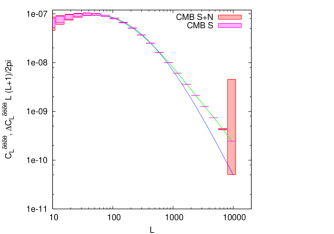
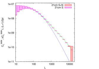
Figure 8.— Displacement field power spectra and sample variance (‘S’) and noise (‘N’) errors. An SKA like experiment might be suited to probe a large dynamical range in the displacement field. The displacement field angular power spectrum with errorbars on the left is for our reference CMB experiment at $f_{\rm sky}=0.8$ and the curves on the right are for 21 cm redshift 6-12 lensing reconstruction using the ”MWA50k” (same collecting area but 10 times higher survey speed than SKA) with $f_{\rm sky}=0.08$.

Finally we would like to estimate the effect foregrounds will have on the estimation of the lensing field suggested here. As pointed out by Madau et al. (1996); Zaldarriaga et al. (2004), fluctuations in the gas at high redshift can be seperated against the much brighter foregrounds (the main source of confusion being galactic and extra-galactic synchrotron), because the former vary rapidly, the latter slowly in frequency. This can be done by fitting various smooth functions to the signal. Morales et al. (2005), Wang et al. (2005), and McQuinn et al. (2005) suggest quadratic or cubic polynomials, but also more complicated functions such as Chebychew polynomials have been proposed. McQuinn et al. (2005) show that this will practically make the first few wavevector modes in the line of sight direction unusable. The exact number of modes that can be used depends of course on the nature of foregrounds, the bandwidth, and the technique of fitting.

On the positive side once a model for foregrounds is given, we can implement this pretty straightforwardly within our formalism by discarding the first few modes $k_{\|}$ (depending on the order of fitting polynomial) in the hierarchy of $C_{l}$’s, compare Figure 3. It is to be expected that a large number of modes still will contribute to the final noise level. This is quantified in Figure 4 where the sum $N_{L}^{-1}=1/\sum_{k_{j>j_{\rm min}}}N_{L,k_{j}\mathcal{L}/(2\pi)}$ is plotted for the two cases $j_{\rm min}=3,10$ meaning that the first 3/10 modes have been discarded in the analysis. The resulting noise levels (short dashed lines) are somewhat higher than the solid line that was obtained from assuming no foregrounds.

6. Discussion

In this paper we have extended the quadratic estimator formalism to use a three dimensional signal as lensing background. 21 cm fluctuations from neutral hydrogen prior and during the epoch of reionization contain an enormous amount of data points. The correlations induced by lensing into this signal can be used to probe the intervening matter fluctuations either on a individual object basis, or statistically to for example probe dark energy models. To describe fluctuations in the neutral fraction, we used an analytic model for the morphology of HII regions to demonstrate the applicability of our method to this regime.

Our estimator should be complete as long as non linearities in the signal (e.g. due to the bubbles) are small. The bulk of the information we use is coming from the neutral phase.

The first generation of experiments is likely not going to be able to image the angular fluctuations in 21 cm needed to measure the lensing effect. However we arrive at good constraints by employing current specifications of the SKA with a flat antenna distribution.

In comparison with the CMB, 21 cm fluctuations have a rather featureless scale invariant unlensed spectrum which leads to a smaller lensing effect. This can be compensated for by using multiple redshift information when probing each individual lens surface. The CMB quadratic estimator sensitivity can actually be beaten this way, for example with an SKA type experiment.

Another possibility would be to combine 21 cm lensing reconstruction with that from other observables, such as the CMB. Similar to combining the latter with galaxy shear surveys, this will improve the constraints on the mass/energy budget or geometry of the universe significantly.

If ambitions in the community of observational and theoretical cosmologists increase in the years to come, and third generation experiments will be scheduled, a new prospect would be the measurement of polarized 21 cm emission. Babich & Loeb (2005) find that Thomson scattering of the quadrupole produced by the reionized universe produces the largest effect and similar to the gains by using CMB polarization, this could make the method suggested in this paper, the three dimensional form of the quadratic estimator, even more promising.

Larger collecting areas and longer observation times also promise to allow 21 cm lensing reconstruction to map out the gravitational potential of individual galaxy clusters. We will attempt to address this topic in a future work.

Appendix A Quadratic estimator applied to a three dimensional observable

We want to observe the three dimensional field $I(\theta,z)$. We assume weak lensing

$${\tilde{\rm I}}(\theta,z)={\rm I}(\theta,z)+\delta\theta\cdot\nabla_{\theta}{\rm I}(\theta,z)+...$$ (A1)

where ${\tilde{\rm I}}(\theta,z)$ is the lensed, ${\rm I}(\theta,z)$ the unlensed field. The Fourier transform of this expression is

$${\tilde{\rm I}}({\bf l},k) = {\rm I}+\int\frac{d^{2}l^{\prime}}{(2\pi)^{2}}(\delta\theta({\bf l}-{\bf l}^{\prime})\cdot i{\bf l}){\rm I}({\bf l}^{\prime},k)$$ (A2)

$$= {\rm I}({\bf l},k)-\int{d^{2}l^{\prime}}{\rm I}({\bf l}^{\prime},k)\phi({\bf l}-{\bf l}^{\prime})({\bf l}-{\bf l}^{\prime})\cdot{\bf l}^{\prime}$$ (A3)

where we have used that $\delta\theta({\bf L})=i{\bf L}\phi({\bf L})$. We are looking for a quadratic estimator $\Phi({\bf L})$ for $\phi({\bf L})$, i.e. of the form

$$\Phi({\bf L})=\int\frac{d^{2}l}{(2\pi)^{2}}\int\frac{dk_{1}}{2\pi}\int\frac{dk_{2}}{2\pi}F({\bf l},k_{1},k_{2},{\bf L})I({\bf l},k_{1})I({\bf L}-{\bf l},k_{2})$$ (A4)

(notice that $F({\bf l},k_{1},k_{2},{\bf L})=F({\bf l},k_{2},k_{1},{\bf L})$). Because $\delta\Phi({\bf L})=\delta\Phi^{*}(-{\bf L})$ it can also be shown that

$$F({\bf l},k_{1},k_{2},{\bf L})=F^{*}(-{\bf l},-k_{1},-k_{2},-{\bf L})$$ (A5)

We want to find $F$ such that it minimizes the variance of $\Phi({\bf L})$ under the condition that its ensemble average recovers the lensing field, $\langle\Phi({\bf L})\rangle_{\rm I}=\phi({\bf L})$. This becomes (to first order in $\phi$)

$$\langle\Phi({\bf L})\rangle_{\rm I} = \int\frac{d^{2}l}{(2\pi)^{2}}\int\frac{dk_{2}}{2\pi}\int\frac{dk_{2}}{2\pi}F({\bf l},k_{1},k_{2},{\bf L})\left[-\langle{\rm I}({\bf l},k_{1})\int\frac{d^{2}l}{(2\pi)^{2}}^{\prime}{\rm I}({\bf l}^{\prime},k_{2})\phi({\bf L}-{\bf l}-{\bf l}^{\prime})\times\right.$$ (A6)

$$\left.\times({\bf L}-{\bf l}-{\bf l}^{\prime})\cdot{\bf l}^{\prime}\rangle-\langle{\rm I}({\bf L}-{\bf l},k_{2})\int\frac{d^{2}l}{(2\pi)^{2}}^{\prime}{\rm I}({\bf l}^{\prime},k_{1})\phi({\bf l}-{\bf l}^{\prime})({\bf l}-{\bf l}^{\prime})\cdot{\bf l}^{\prime}\rangle\right]$$

$$= -\int\frac{d^{2}l}{(2\pi)^{2}}\int\frac{dk_{1}}{2\pi}\int\frac{dk_{2}}{2\pi}F({\bf l},k_{1},k_{2},{\bf L})\left[\int\frac{d^{2}l}{(2\pi)^{2}}^{\prime}(2\pi)^{2}\delta({\bf l}+{\bf l}^{\prime})(2\pi)\delta(k_{1}+k_{2}){\rm P}_{l,k}\times\right.$$

$$\left.\times\phi({\bf L}-{\bf l}-{\bf l}^{\prime})({\bf L}-{\bf l}-{\bf l}^{\prime})\cdot{\bf l}^{\prime}+\int\frac{d^{2}l}{(2\pi)^{2}}^{\prime}(2\pi)^{2}\delta({\bf L}-{\bf l}+{\bf l}^{\prime})(2\pi)\delta(k_{1}+k_{2}){\rm P}_{L-l,k}\phi({\bf l}-{\bf l}^{\prime})({\bf l}-{\bf l}^{\prime})\cdot{\bf l}^{\prime}\right]$$

$$= -\int\frac{d^{2}l}{(2\pi)^{2}}\int\frac{dk_{1}}{2\pi}\int\frac{dk_{2}}{2\pi}F({\bf l},k_{1},k_{2},{\bf L})(2\pi)\delta(k_{1}+k_{2})\left[{\rm P}_{l,k}\phi({\bf L}){\bf L}\cdot(-{\bf l})+{\rm P}_{L-l,k}\phi({\bf L}){\bf L}\cdot(-({\bf L}-{\bf l}))\right]$$

$$= \int\frac{d^{2}l}{(2\pi)^{2}}\int\frac{dk_{1}}{2\pi}\int\frac{dk_{2}}{2\pi}F({\bf l},k_{1},k_{2},{\bf L})(2\pi)\delta(k_{1}+k_{2})\left[{\rm P}_{l,k}\phi({\bf L}){\bf L}\cdot{\bf l}+{\rm P}_{L-l,k}\phi({\bf L}){\bf L}\cdot({\bf L}-{\bf l})\right]\,,$$

where e.g. ${\rm P}_{l,k}$ is the power in a mode with angular component $l$ and radial component $k$. With the requirement that $\langle\Phi({\bf L})\rangle_{\rm I}=\phi({\bf L})$ this leads to the normalization condition

$$\int\frac{d^{2}l}{(2\pi)^{2}}\int\frac{dk_{1}}{2\pi}\int\frac{dk_{2}}{2\pi}F({\bf l},k_{1},k_{2},{\bf L})(2\pi)\delta^{D}(k_{1}+k_{2})\left[{\rm P}_{l,k}{\bf L}\cdot{\bf l}+{\rm P}_{L-l,k}{\bf L}\cdot({\bf L}-{\bf l})\right]=1$$ (A7)

The next step is to minimize the variance

$$\langle||\Phi({\bf L})||^{2}\rangle_{\tilde{\rm I}} = \int\frac{d^{2}l}{(2\pi)^{2}}\int\frac{dk_{1}}{2\pi}\int\frac{dk_{2}}{2\pi}\int\frac{d^{2}l}{(2\pi)^{2}}^{\prime}\int\frac{dk_{1}}{2\pi}^{\prime}\int\frac{dk_{2}}{2\pi}^{\prime}F({\bf l},k_{1},k_{2},{\bf L})F^{*}({\bf l}^{\prime},k_{1}^{\prime},k_{2}^{\prime},{\bf L}^{\prime})\times$$ (A8)

$$\hskip 165.02606pt\times\langle{\tilde{\rm I}}({\bf l},k_{1}){\tilde{\rm I}}({\bf L}-{\bf l},k_{2}){\tilde{\rm I}}({\bf l}^{\prime},k_{1}^{\prime}){\tilde{\rm I}}({\bf L}-{\bf l}^{\prime},k_{2}^{\prime})\rangle$$

$$= \int\int\int\int\int\int F({\bf l},k_{1},k_{2},{\bf L})F^{*}({\bf l}^{\prime},k_{1}^{\prime},k_{2}^{\prime},{\bf L}^{\prime})(2\pi)^{2}\delta({\bf l}-{\bf l}^{\prime})(2\pi)\delta(k_{1}-k_{1}^{\prime}){\tilde{\rm P}^{\rm tot}}_{l,k_{1}}\times$$

$$\hskip 165.02606pt\times(2\pi)^{2}\delta({\bf l}^{\prime}-{\bf l})(2\pi)\delta(k_{2}-k_{2}^{\prime}){\tilde{\rm P}^{\rm tot}}_{L-l,k_{2}}$$

$$+\int\int\int\int\int\int F({\bf l},k_{1},k_{2},{\bf L})F^{*}({\bf l}^{\prime},k_{1}^{\prime},k_{2}^{\prime},{\bf L}^{\prime})(2\pi)^{2}\delta({\bf l}-{\bf L}+{\bf l}^{\prime})(2\pi)\delta(k_{1}-k_{2}^{\prime}){\tilde{\rm P}^{\rm tot}}_{l,k_{1}}\times$$

$$\hskip 165.02606pt\times(2\pi)^{2}\delta({\bf L}-{\bf l}-{\bf l}^{\prime})(2\pi)\delta(k_{2}-k_{1}^{\prime}){\tilde{\rm P}^{\rm tot}}_{L-l,k_{2}}$$

$$= \int\frac{d^{2}l}{(2\pi)^{2}}\int\frac{dk_{1}}{2\pi}\int\frac{dk_{2}}{2\pi}(2\pi)^{2}\delta(0)F({\bf l},k_{1},k_{2},{\bf L})F^{*}({\bf l}^{\prime},k_{1}^{\prime},k_{2}^{\prime},{\bf L}^{\prime}){\tilde{\rm P}^{\rm tot}}_{l,k_{1}}{\tilde{\rm P}^{\rm tot}}_{L-l,k_{2}}$$

$$+\int\frac{d^{2}l}{(2\pi)^{2}}\int\frac{dk_{1}}{2\pi}\int\frac{dk_{2}}{2\pi}(2\pi)^{2}\delta(0)F({\bf l},k_{1},k_{2},{\bf L})F^{*}({\bf L}-{\bf l}^{\prime},k_{2}^{\prime},k_{1}^{\prime},{\bf L}^{\prime}){\tilde{\rm P}^{\rm tot}}_{l,k_{1}}{\tilde{\rm P}^{\rm tot}}_{L-l,k_{2}}$$

but from A4 we see with the substitution ${\bf L}-{\bf l}\rightarrow{\bf l}$ that $F^{*}({\bf L}-{\bf l},k_{2},k_{1},{\bf L})=F^{*}({\bf l},k_{1},k_{2},{\bf L})$ hence

$$\langle||\Phi({\bf L})||^{2}\rangle=2(2\pi)^{2}\delta(0)\int\frac{d^{2}l}{(2\pi)^{2}}\int\frac{dk_{1}}{2\pi}\int\frac{dk_{2}}{2\pi}F({\bf l},k_{1},k_{2},{\bf L})F^{*}({\bf l},k_{1},k_{2},{\bf L}){\tilde{\rm P}^{\rm tot}}_{l,k_{1}}{\tilde{\rm P}^{\rm tot}}_{l,k_{2}}\,.$$ (A9)

Both real and imaginary part of $||F||^{2}=F_{R}^{2}+F_{I}^{2}$ contribute to this variance, however the condition for the minimization will only pick out the real part. The solution is found by minimizing the function

$$\langle||\Phi({\bf L})||^{2}\rangle-A_{R}\times(\,{\rm Equation}\,\ref{eq:normcond})$$ (A10)

with respect to $F$, where $A_{R}$ is a Lagrangian multiplier. In steps,

$$\frac{\partial(\,{\rm Eq.}\,\ref{eq:normcond})}{\partial F({\bf l},k_{1},k_{2},{\bf L})}=A_{R}\frac{d^{2}l}{(2\pi)^{2}}\frac{dk_{1}}{2\pi}\frac{dk_{2}}{2\pi}(2\pi)\delta^{D}(k_{1}+k_{2})[{\rm P}_{l,k}{\bf L}\cdot{\bf l}+{\rm P}_{L-l,k}{\bf L}\cdot({\bf L}-{\bf l})]$$ (A11)

and

$$\frac{\partial\langle||\Phi({\bf L})||^{2}\rangle}{\partial F({\bf l},k_{1},k_{2},{\bf L})}=2(2\pi)^{2}\delta(0)\frac{d^{2}l}{(2\pi)^{2}}\frac{dk_{1}}{2\pi}\frac{dk_{2}}{2\pi}2F_{R}({\bf l},k_{1},k_{2},{\bf L}){\tilde{\rm P}^{\rm tot}}_{l,k_{1}}{\tilde{\rm P}^{\rm tot}}_{L-l,k_{2}}$$ (A12)

so

$$F_{R}({\bf l},k_{1},k_{2},{\bf L})=A_{R}(2\pi)\delta^{D}(k_{1}+k_{2})\frac{[{\rm P}_{l,k}{\bf L}\cdot{\bf l}+{\rm P}_{L-l,k}{\bf L}\cdot({\bf L}-{\bf l})]}{{\tilde{\rm P}^{\rm tot}}_{l,k_{1}}{\tilde{\rm P}^{\rm tot}}_{L-l,k_{2}}}$$ (A13)

and by inserting this into the normalization condition A7 we get that

$$A_{R}=\frac{1}{\sum_{k}\int\frac{d^{2}l}{(2\pi)^{2}}\frac{[{\rm P}_{l,k}{\bf L}\cdot{\bf l}+{\rm P}_{L-l,k}{\bf L}\cdot({\bf L}-{\bf l})]^{2}}{{\tilde{\rm P}^{\rm tot}}_{l,k_{1}}{\tilde{\rm P}^{\rm tot}}_{L-l,k_{2}}}}\,.$$ (A14)

By using Equation A13 we find that the variance becomes

$$\langle||\Phi(L)||^{2}\rangle = 2(2\pi)^{2}\delta(0)\int\frac{d^{2}l}{(2\pi)^{2}}\int\frac{dk_{1}}{2\pi}\int\frac{dk_{2}}{2\pi}{\tilde{\rm P}^{\rm tot}}_{l,k_{1}}{\tilde{\rm P}^{\rm tot}}_{L-l,k_{2}}F_{R}^{2}$$

$$= 2(2\pi)^{2}\delta(0)A_{R}^{2}\int\frac{d^{2}l}{(2\pi)^{2}}\int\frac{dk_{1}}{2\pi}\int\frac{dk_{2}}{2\pi}[(2\pi)\delta(k_{1}+k_{2})]^{2}\frac{[{\rm P}_{l,k}\,{\bf L}\cdot{\bf l}+{\rm P}_{L-l,k}\,{\bf L}\cdot({\bf L}-{\bf l})]^{2}}{{\tilde{\rm P}^{\rm tot}}_{l,k}\,{\tilde{\rm P}^{\rm tot}}_{L-l,k}}$$

Using $(2\pi)\delta^{D}(0)=\frac{2\pi}{dk}$ and $\int\frac{dk}{2\pi}\frac{2\pi}{dk}\rightarrow\sum_{k}$, this becomes

$$\langle||\Phi(L)||^{2}\rangle = 2(2\pi)^{2}\delta(0)A_{R}^{2}\sum_{k}\int\frac{d^{2}l}{(2\pi)^{2}}\frac{[{\rm P}_{l,k}\,{\bf L}\cdot{\bf l}+{\rm P}_{L-l,k}\,{\bf L}\cdot({\bf L}-{\bf l})]^{2}}{{\tilde{\rm P}^{\rm tot}}_{l,k}\,{\tilde{\rm P}^{\rm tot}}_{L-l,k}}$$ (A17)

$$= 2(2\pi)^{2}\delta(0)A_{R}^{2}\frac{2}{A_{R}}$$

$$= (2\pi)^{2}\delta(0)\frac{1}{\sum_{k}\int\frac{[{\rm P}_{l,k}{\bf L}\cdot{\bf l}+{\rm P}_{L-l,k}{\bf L}\cdot({\bf L}-{\bf l})]^{2}}{2\,{\tilde{\rm P}^{\rm tot}}_{l,k}{\tilde{\rm P}^{\rm tot}}_{L-l,k}}}$$

With the definition of the noise power spectrum $N_{L}^{\Phi}$,

$$\langle\Phi({\bf L})\Phi^{*}({\bf L}^{\prime})\rangle = (2\pi)^{2}\delta^{D}({\bf L}-{\bf L}^{\prime})N_{L}^{\Phi}$$ (A18)

$$\,{\rm or}\,\langle||\Phi(L)||^{2}\rangle = (2\pi)^{2}\delta^{D}(0)N_{L}^{\Phi}$$ (A19)

it follows that

$$N_{L}^{\Phi}=\frac{1}{\sum_{k}\int\frac{d^{2}l}{(2\pi)^{2}}\frac{[{\rm P}_{l,k}\,{\bf L}\cdot{\bf l}+{\rm P}_{L-l,k}\,{\bf L}\cdot({\bf L}-{\bf l})]^{2}}{2{\tilde{\rm P}^{\rm tot}}_{l,k}\,{\tilde{\rm P}^{\rm tot}}_{L-l,k}}}$$ (A20)

and since the variances of estimator $D$ of the displacement $\langle D\rangle_{\rm ens.}=\delta\theta$ and $\Phi$ are just related by $\langle||D({\bf L})||^{2}\rangle=L^{2}\langle||\Phi({\bf L})||^{2}\rangle$ we obtain

$$N_{L}^{D} = \frac{1}{\sum_{k}\frac{1}{L^{2}}\int\frac{d^{2}l}{(2\pi)^{2}}\frac{[{\rm P}_{l,k}{\bf L}\cdot{\bf l}+{\rm P}_{L-l,k}{\bf L}\cdot({\bf L}-{\bf l})]^{2}}{2{\tilde{\rm P}^{\rm tot}}_{l,k}{\tilde{\rm P}^{\rm tot}}_{L-l,k}}}$$ (A21)

$$= \frac{1}{\sum_{k}N_{L,k}^{-1}}$$

so we have justified that we can simply sum over seperate k modes to arrive at our final lensing noise.

References

- Amblard et al. (2004) Amblard, A., Vale, C., & White, M. J. 2004, New Astron., 9, 687
- Babich & Loeb (2005) D. Babich and A. Loeb, Astrophys. J. 635, 1 (2005) [arXiv:astro-ph/0505358].
- Barkana & Loeb (2005) Barkana, R. & Loeb, A. 2005, Astrophys. J., 624, L65
- Ciardi & Madau (2003) Ciardi, B. & Madau, P. 2003, Astrophys. J., 596, 1
- Cooray (2004) Cooray, A. R. 2004, New Astron., 9, 173
- Fan et al. (2005) X. H. Fan et al., arXiv:astro-ph/0512082.
- Field (1958) Field, G. B. 1958, Proc. IRE, 46, 240
- Field (1959) Field, G. B. 1959, ApJ, 129, 525
- Furlanetto et al. (2004a) Furlanetto, S., Sokasian, A., & Hernquist, L. 2004a, Mon. Not. Roy. Astron. Soc., 347, 187
- Furlanetto et al. (2004b) Furlanetto, S., Zaldarriaga, M., & Hernquist, L. 2004b, Astrophys. J. 613, 1 (2004)
- Gunn & Peterson (1965) Gunn, J. E. & Peterson, B. A. 1965, Astrophys. J., 142, 1633
- Hirata & Seljak (2002) C. M. Hirata and U. Seljak, Phys. Rev. D 67, 043001 (2003)
- Hirata & Seljak (2003) Hirata, C. M. & Seljak, U. 2003, Phys. Rev., D68, 083002
- Hu (2001a) Hu, W. 2001a, Phys. Rev., D64, 083005
- Hu (2001b) Hu, W. 2001b, Astrophys. J., 557, L79
- Hu (2002) Hu, W. 2002, Phys. Rev., D65, 023003
- Hu & Holder (2003) Hu, W. & Holder, G. P. 2003, Phys. Rev., D68, 023001
- Hu & Okamoto (2002) Hu, W. & Okamoto, T. 2002, Astrophys. J., 574, 566
- Knox (1996) Knox, L. 1996, Astrophys, J., 480, 72
- Kosowsky (2003) Kosowsky, A. 2003, New Astron. Rev., 47, 939
- Loeb & Zaldarriaga (2004) Loeb, A. & Zaldarriaga, M. 2004, Phys. Rev. Lett., 92, 211301
- Madau et al. (1996) Madau, P., Meiksin, A., & Rees, M. J. 1996
- Mandel & Zaldarriaga (2005) Mandel, K. & Zaldarriaga, M. 2005, arXiv:astro-ph/0512218
- McQuinn et al. (2005) M. McQuinn, O. Zahn, M. Zaldarriaga, L. Hernquist and S. R. Furlanetto, 2005, arXiv:astro-ph/0512263.
- Miralda-Escude et al. (1998) Miralda-Escude, J., Haehnelt, M., & Rees, M. J. 1998, Astrophys. J., 530, 1
- Morales (2005) Morales, M. F. 2005, Astrophys. J., 619, 678
- Morales et al. (2005) Morales, M. F., Bowman, J. D., & Hewitt, J. N. 2005, Astrophys. J., 648 in press.
- Oxley et al. (2004) Oxley, P. et al. 2004, Proc. SPIE Int. Soc. Opt. Eng., 5543, 320
- Page et al. (2006) Page, L. et al., arXiv:astro-ph/0603450.
- Pen (2004) Pen, U.-L. 2004, New Astron., 9, 417
- Pen et al. (2004) Pen, U.-L., Wu, X.-P., & Peterson, J. 2004, American Astronomical Society
- Ruhl et al. (2004) Ruhl, J. et al. 2004, A. A. 2004. Proceedings of the SPIE, Volume 5498, pp. 11-29 (2004)., 11–29
- Spergel et al. (2006) Spergel, D. N. et al., arXiv:astro-ph/0603449.
- Seljak & Hirata (2004) Seljak, U. & Hirata, C. M. 2004, Phys. Rev., D69, 043005
- Seljak & Zaldarriaga (1996) Seljak, U. & Zaldarriaga, M. 1996, Astrophys. J., 469, 437
- Sigurdson & Cooray (2005) Sigurdson, K. & Cooray, A. 2005, Phys. Rev. Lett., 95, 211303
- Smith et al. (2003) Smith, R. E. et al. 2003, Mon. Not. Roy. Astron. Soc., 341, 1311
- Sokasian et al. (2003) Sokasian, A., Abel, T., Hernquist, L., & Springel, V. 2003, Mon. Not. Roy. Astron. Soc., 344, 607
- Sunyaev & Zeldovich (1980) Sunyaev, R. A. & Zeldovich, Y. B. 1980, Mon. Not. Roy. Astron. Soc., 190, 413
- Wang et al. (2005) Wang, X.-M., Tegmark, M., Santos, M., & Knox, L. 2005, arXiv:astro-ph/0501081
- White et al. (1999) White, M. J., Carlstrom, J. E., & Dragovan, M. 1999, Astrophys. J., 514, 12
- Wouthuysen (1952) Wouthuysen, S. A., Astronomical Journal, Vol. 52, p. 31
- Wyithe & Loeb (2004) Wyithe, J. S. B. & Loeb, A. 2004, arXiv:astro-ph/0409412
- Wyithe et al. (2005) Wyithe, J. S. B., Loeb, A., & Carilli, C. 2005, Astrophys. J., 628, 575
- Zahn et al. (2005) Zahn, O., Zaldarriaga, M., Hernquist, L., & McQuinn, M. 2005, Astrophys. J., 630, 657
- Zaldarriaga (1997) Zaldarriaga, M. 1997, Phys. Rev., D55, 1822
- Zaldarriaga et al. (2004) Zaldarriaga, M., Furlanetto, S. R., & Hernquist, L. 2004, Astrophys. J., 608, 622
- Zhang & Pen (2005) Zhang, P. & Pen, U.-L. 2005, arXiv:astro-ph/0506740