Simulating Radiating and Magnetized Flows in Multi-Dimensions with ZEUS-MP

Abstract

This paper describes ZEUS-MP, a multi-physics, massively parallel, message-passing implementation of the ZEUS code. ZEUS-MP differs significantly from the thoroughly documented ZEUS-2D code, the completely undocumented (in peer-reviewed literature) ZEUS-3D code, and a marginally documented “version 1” of ZEUS-MP first distributed publicly in 1999. ZEUS-MP offers an MHD algorithm which is better suited for multidimensional flows than the ZEUS-2D module by virtue of modifications to the Method of Characteristics scheme first suggested by Hawley & Stone (1995). This MHD module is shown to compare quite favorably to the TVD scheme described by Ryu et al. (1998). ZEUS-MP is the first publicly-available ZEUS code to allow the advection of multiple chemical (or nuclear) species. Radiation hydrodynamic simulations are enabled via an implicit flux-limited radiation diffusion (FLD) module. The hydrodynamic, MHD, and FLD modules may be used, singly or in concert, in one, two, or three space dimensions. Additionally, so-called “1.5-D” and “2.5-D” grids, in which the “half-D” denotes a symmetry axis along which a constant but non-zero value of velocity or magnetic field is evolved, are supported. Self gravity may be included either through the assumption of a $GM/r$ potential or a solution of Poisson’s equation using one of three linear solver packages (conjugate-gradient, multigrid, and FFT) provided for that purpose. Point-mass potentials are also supported.

Because ZEUS-MP is designed for large simulations on parallel computing platforms, considerable attention is paid to the parallel performance characteristics of each module in the code. Strong-scaling tests involving pure hydrodynamics (with and without self-gravity), MHD, and RHD are performed in which large problems (256³ zones) are distributed among as many as 1024 processors of an IBM SP3. Parallel efficiency is a strong function of the amount of communication required between processors in a given algorithm, but all modules are shown to scale well on up to 1024 processors for the chosen fixed problem size.

1. Introduction

Since their formal introduction in the literature, the ZEUS simulation codes have enjoyed widespread use in the numerical astrophysics community, having been applied to such topics as planetary nebulae (García-Segura et al., 1999), molecular cloud turbulence (Mac Low, 1999), solar magnetic arcades (Low & Manchester, 2000), and galactic spiral arm formation (Martos et al., 2004a, b). The numerical methods used in the axisymmetric ZEUS-2D code are documented in an often-cited trio of papers (Stone & Norman, 1992a, b; Stone et al., 1992b) well familiar to the computational astrophysics community. A reasonable first question to ask regarding this report might therefore be, “why write another ZEUS ‘method’ paper?” The first reason is that the code we describe in this paper, ZEUS-MP, is a significantly different code when compared to the highly-documented ZEUS-2D code, the completely undocumented (in peer-reviewed literature) ZEUS-3D code, and a marginally documented “version 1” of ZEUS-MP made publicly available in 1999. The new version of ZEUS-MP we present is the first ZEUS code to unite 3D hydrodynamics (HD) and 3D magnetohydrodynamics (MHD) with implicit flux-limited radiation diffusion (FLD) and self-gravity in a software framework designed for execution on massively parallel architectures. This last feature anticipates a second major reason for offering a new method paper: the computing hardware landscape in which numerical astrophysicists operate has changed enormously since the ZEUS-2D trilogy was published. The enormous increase in computer processor speed and available memory has brought with it a new paradigm for computing in which large simulations are distributed across many (often hundreds to thousands) of parallel processors; this new environment has spawned additional figures of merit, such as parallel scalability, by which modern numerical algorithms must be judged. A major component of this paper is the demonstration of the suitability of ZEUS-MP’s algorithms, both new and familiar, for parallel execution on thousands of processors.

In addition to describing the many new features and capabilities provided in  ZEUS-MP, this paper fills significant gaps in the evolution history of the MHD and radiation modules offered in predecessors of ZEUS-MP. These gaps were partially a consequence of the evolution of the ZEUS series. The first code formally named ZEUS was developed by David Clarke  (Clarke, 1988; Clarke et al., 1986) for MHD simulations of radio jets. Thereafter, continued development of the ZEUS method proceeded along two parallel tracks. One track resulted in the release of the ZEUS-2D code, which solves the equations of self-gravitating radiation magnetohydrodynamics in two or 2.5 dimensions. (“2.5-D” denotes a problem computed in 2 spatial dimensions involving the 3-component of a vector quantity, such as velocity, that is invariant along the 3-axis but variable along the 1- and 2-axes.) The creation of ZEUS-2D occasioned the development and incorporation of several new algorithms, including (1) a covariant formulation, allowing simulations in various coordinate geometries; (2) a tensor artificial viscosity; (3) a new, more accurate MHD algorithm (MOCCT) combining the Constrained Transport algorithm (Evans & Hawley, 1988) with a Method Of Characteristics treatment for Alfvén waves; and (4) a variable tensor Eddington factor (VTEF) solution for the equations of radiation hydrodynamics (RHD). The VTEF radiation module was described in Stone et al. (1992b) but not included in the version of ZEUS-2D offered for public distribution. An implicit FLD-based RHD module was publicly distributed with ZEUS-2D but never documented in a published report. (A draft of a technical report describing the 2-D FLD module is available on the World Wide Web.) The VTEF module described in Stone et al. (1992b) was later modified to incorporate a different matter-radiation coupling scheme, Eddington tensors computed from a time-dependent solution to the radiation transfer equation, and parallelization over two space dimensions and one angle cosine. This new VTEF code was coupled to an early version of ZEUS-MP and used to compare VTEF solutions to FLD results for test problems featuring strongly beamed radiation fields. This work was published by Hayes & Norman (2003), but as before the VTEF module remained reserved for private use. ZEUS-MP as described herein provides an updated FLD module designed for all dimensionalities and geometries in a parallel computing environment. This paper documents our new module at a level of detail which should aid users of both ZEUS-MP and the public ZEUS-2D code.

The second track resulted in the release of ZEUS-3D, the first ZEUS code capable of three-dimensional simulations. Written for the Cray-2 supercomputer by David Clarke, ZEUS-3D physics options included hydrodynamics, MHD, self-gravity, and optically thin radiative cooling. ZEUS-3D was the first ZEUS code with parallel capability, accomplished using Cray Autotasking compiler directives. The ZEUS-3D MHD module differed from that described in the ZEUS-2D papers with regard to both dimensionality and method: the MOC treatment of Alfvén waves was modified to incorporate the improvements introduced by John Hawley and James Stone (Hawley & Stone, 1995). This modified “HSMOCCT” method is the basis for the MHD module adopted in ZEUS-MP.

Roughly speaking, ZEUS-MP encapsulates a qualitative union of the methods provided by the public ZEUS-2D and ZEUS-3D codes and enlarges upon them with new capabilities and solution techniques. The first public release of ZEUS-MP included HD, MHD, and self gravity, but was written exclusively for 3-D simulations, excluding at one stroke a long menu of worthy 2-D research applications and erecting an inconvenient barrier to expedient code testing. The new version we describe offers a substantially extended menu of physics, algorithm, and dimensionality options. The HD, MHD, and RHD modules accommodate simulations in 1, 1.5, 2, 2.5, and 3 dimensions. Arbitrary equations of state are supported; gamma-law and isothermal equations of state are provided. ZEUS-MP is the first ZEUS code to allow multi-species fluids to be treated; this is achieved with the addition of a concentration field array dimensioned for an arbitrary number of fluids. An implicit flux-limited photon diffusion module is included for RHD problems. As noted previously, the implicit FLD solution is based upon the method adopted for the public version of ZEUS-2D but has been extended to three dimensions. In addition, the FLD module sits atop a scalable linear system solver using the conjugate gradient (CG) method (Barret et al., 1994). Supplementing the FLD driver is an opacity module offering simple density and temperature-dependent power-law expressions for absorption and scattering coefficients; additional user-supplied modules (such as tabular data sets) are easily accommodated. Self-gravity is included in several ways: (1) spherical gravity (GM/r) is adopted for one-dimensional problems and may also be used in two dimensions; (2) two parallel Poisson solvers are included for problems with Neumann or Dirichlet boundary conditions in Cartesian or curvilinear coordinates, and (3) a fast Fourier Transform (FFTw) package is provided for problems with triply-periodic boundaries. In addition to self-gravity, a simple point-mass external potential may be imposed in spherical geometry.

While the ZEUS code line has evolved significantly, this process has not occurred in a vacuum. Indeed, the past decade has seen the emergence of several new MHD codes based upon Godunov methods (Ryu et al., 1998; Londrillo & Del Zanna, 2000; Londrillo & del Zanna, 2004; Balsara, 2004; Gardiner & Stone, 2005). Godunov-type schemes are accurate to second order in both space and time, are automatically conservative, and possess superior capability for resolving shock fronts when compared to ZEUS-type schemes at identical resolution. These advances, coupled with ZEUS’s lower-order rate of convergence with numerical resolution (Stone et al., 1992a), and further with recent observations (Falle, 2002) of vulnerabilities in the ZEUS-2D implementation of MOCCT might lead one to ask whether a new ZEUS code has a strong potential for future contributions of significance in areas of current astrophysical interest. We argue this point in the affirmative on two fronts. While we acknowledge that the ZEUS method possesses (as do all numerical methods) weaknesses which bound its scope of applicability, we note the encouraging comparisons (Stone & Gardiner, 2005) of simulation results computed with Athena, an unsplit MHD code coupling PPM hydrodynamics to Constrained Transport, to ZEUS results in problems of supersonic MHD turbulence in 3D, and in shearing-box simulations of the magneto-rotational instability in two and three dimensions. The authors confirm the reliability of the ZEUS results and note that the numerical dissipation in Athena is equivalent to that of ZEUS at a grid resolution of about 1.5 along each axis. In a similar vein, we examine a standard 2-D MHD test problem, due to Orszag & Tang (1979), in which the results from ZEUS-MP are found to compare quite favorably with those from the TVD code described in Ryu et al. (1998) and with results from different upwind Godunov codes presented by Dai & Woodward (1998) and Londrillo & Del Zanna (2000).

A second cause for optimism of ZEUS’s future arises from the versatility inherent in ZEUS-MP’s design. As this paper demonstrates, a wide variety of physics modules are easily implemented within ZEUS-MP’s design framework. Additionally, different solution techniques for treating the same physics (self-gravity is an excellent example) are almost trivially accommodated. The theme of this paper is, therefore: physics, flexibility, and parallel performance. To demonstrate these traits we organize the paper as follows: the presentation begins by writing the fluid equations solved by ZEUS-MP in  section 2; section 3 provides a largely descriptive overview of the various numerical methods used to solve these equations on a discrete mesh. Sections 4 and 5 present two groups of test problems. Section 4 provides a suite of tests to verify the correctness of the various physics modules. Section 5 examines a quartet of 3-D problems which measure performance on a massively parallel computer.

The main body of the paper is concluded with a summary in section 6. Full documentation of the finite-difference formulae describing hydrodynamic, magnetohydrodynamic, and radiation hydrodynamic evolution in three dimensions is provided in a series of appendices. These appendices are preceded by a tabular “code map” (Table 7) in appendix A associating the discrete equations written in appendices B-E with the subroutines in ZEUS-MP that compute them. We offer this as an aid to users wishing to familiarize themselves with the code and to code developers who desire to implement their own versions or improve upon what is currently offered in ZEUS-MP. The HD, MHD, and FLD modules are detailed in appendices B, C, and D, respectively. Appendix E documents the 3-D linearized form of Poisson’s equation expressed in covariant grid coordinates, and details of our parallel implementation techniques and strategies are given in appendix F.

2. The Physical Equations

Our description of the physical state of a fluid element is specified by the following set of fluid equations relating the mass density ($\rho$), velocity (${\bf v}$), gas internal energy density (${\rm e}$), radiation energy density (${\rm E}$), radiation flux (${\bf F}$), and magnetic field strength (${\bf B}$):

$${D\rho\over Dt}\ +\ \rho{\bf\nabla\cdot}{\bf v}\ =\ 0;$$ (1)

$$\rho{D{\bf v}\over Dt}\ =\ -{\bf\nabla}{\rm p}\ +\ \left(\chi\over c\right){\bf F}\ +\ {1\over 4\pi}\left({\bf\nabla\times}{\bf B}\right){\bf\times}{\bf B}\ -\ {\rho{\bf\nabla}\Phi};$$ (2)

$$\rho{D\over Dt}\left({{\rm e}\over\rho}\right)\ +\ {\rm p}{\bf\nabla\cdot}{\bf v}\ =\ c{\kappa_{\rm E}}{\rm E}\ -\ 4\pi{\kappa_{\rm P}}{\rm B_{p}};$$ (3)

$$\rho{D\over Dt}\left({{\rm E}\over\rho}\right)\ +\ {\bf\nabla\cdot}{\bf F}\ +\ {\bf\nabla}{\bf v}:{\bf P}\ =\ 4\pi{\kappa_{\rm P}}{\rm B_{p}}\ -\ c{\kappa_{\rm E}}{\rm E};$$ (4)

$${\partial{\bf B}\over\partial t}\ =\ {\bf\nabla\times}\left({\bf v}{\bf\times}{\bf B}\right).$$ (5)

The Lagrangean (or comoving) derivative is given by the usual definition:

$${D\over Dt}\ \equiv\ {\partial\over\partial t}\ +\ {\bf v}\cdot\nabla$$ (6)

The four terms on the RHS of the gas momentum equation (2) denote forces to due thermal pressure gradients, radiation stress, magnetic Lorentz acceleration, and the gravitational potential, respectively. The RHS of (3) gives source/sink terms due to absorption/emission of radiant energy. Each term serves an inverse role on the RHS of (4). In (3), ${\rm B_{p}}$ denotes the Planck function:

$${\rm B_{p}}\ =\ {\sigma\over\pi}{\rm T}^{4},$$ (7)

where T is the local material temperature. Equations (3) and (4) are also functions of flux-mean, Planck-mean, and energy-mean opacities, which are formally defined as

$$\chi\ =\ {1\over{\bf F}}\int_{0}^{\infty}\chi(\nu){\bf F}(\nu)d\nu,$$ (8)

$${\kappa_{\rm P}}\ =\ {1\over{\rm B_{p}}}\int_{0}^{\infty}\chi(\nu){\rm B_{p}}(\nu)d\nu,$$ (9)

$${\kappa_{\rm E}}\ =\ {1\over E}\int_{0}^{\infty}\chi(\nu)E(\nu)d\nu.$$ (10)

In the simple problems we discuss in this paper, the three opacities are computed from a single expression, differing only in that ${\kappa_{\rm E}}$ and ${\kappa_{\rm P}}$ are defined at zone centers and $\chi$ is computed at zone faces. In general, however, independent expressions or data sets for the three opacities are trivially accommodated in our discrete representation of the RHD equations.

We compute the radiation flux, ${\bf F}$, according to the diffusion approximation:

$${\bf F}\ =\ -\left(c\Lambda_{\rm E}\over\chi\right){\bf\nabla}{\rm E},$$ (11)

where we have introduced a flux-limiter ($\Lambda_{\rm E}$) to ensure a radiation propagation speed that remains bounded by the speed of light (c) in transparent media. Attenuation of the flux is regulated by the total extinction coefficient, $\chi$, which in general may include contributions from both absorption and scattering processes.

Equation (4) also includes a term involving the radiation stress tensor, ${\bf P}$. In general, ${\bf P}$ is not known a priori and must be computed from a solution to the radiative transfer equation. In the VTEF methods described in Stone et al. (1992b) and Hayes & Norman (2003), ${\bf P}$ is written as the product of the (known) radiation energy, E, and an (unknown) tensor quantity, ${\bf f}$:

$${\bf P}\ =\ {\bf f}{\rm E}.$$ (12)

A solution for ${\bf f}$ may be derived from a formal solution to the radiative transfer equation (Mihalas, 1978) or may be approximated analytically. For the RHD implementation in ZEUS-MP, we follow the latter approach, adopting the expression for ${\bf f}$ given by equation (13) in Turner & Stone (2001):

$${\bf f}\ =\ {1\over 2}\left(1-f\right){\bf I}\ +\ {1\over 2}\left(3f-1\right)\hat{\bf n}\hat{\bf n},$$ (13)

where $\hat{\bf n}={\bf\nabla}{\rm E}/\mid{\bf\nabla}{\rm E}\mid$, I is the unit tensor, and $f$ is a scalar “Eddington factor” expressed as a function of the flux limiter, $\Lambda_{\rm E}$, and E as

$$f\ =\ \Lambda_{\rm E}\ +\ \left(\Lambda_{\rm E}\mid{\bf\nabla}{\rm E}\mid\over{\chi{\rm E}}\right)^{2}$$ (14)

The RHD equations are accurate only to order unity in ${\bf v}/c$ (Mihalas & Mihalas, 1984), consistent with the radiation modules described in Stone et al. (1992b), Turner & Stone (2001), and Hayes & Norman (2003). The assumption of local thermodynamic equilibrium is reflected in our adoption of the Planck function in equations (3) and (4) evaluated at the local material temperature; our use of the FLD approximation gives rise to equation (11) and is discussed further in § 3.3.

Evolution of the magnetic field (5) is constrained by the assumption of ideal MHD. We are therefore, in common with previous public ZEUS codes, assuming wave modes which involve fluid motions but no charge separation. This equation for ${\bf B}$ also assumes zero resistivity, a valid approximation in astrophysical environments where the degree of ionization is sufficiently high to ensure a rapid collision rate between charged and neutral particles and thus strong coupling between the two. There exist astrophysical environments where this assumption is expected to break down (e.g. the cores of cold, dense molecular clouds), in which case an algorithm able to distinguish the dynamics of ionized and neutral particles is required. Stone (1999) published extensions to the ZEUS MHD algorithm to treat nonideal phenomena such as Ohmic dissipation and partially ionized plasmas where the ionic and neutral components of the fluid are weakly coupled via a collisional drag term. Incorporation of these algorithmic extensions into ZEUS-MP is currently left as an exercise to the interested user, but may be undertaken for a future public release.

The gravitational potential $\Phi$ appearing in (2) is computed from a solution to Poisson’s equation:

$${\bf\nabla}{{}^{2}}\Phi\ =\ {4\pi{\rm G}\rho}.$$ (15)

Our various techniques for solving (15) are described in §3.4; the linear system which arises from discretizing (15) on a covariant coordinate mesh is derived in appendix E.

Our fluid equations are closed with an equation of state (EOS) expressing the thermal pressure as a function of the internal gas energy. The dynamic test problems considered in this paper adopt a simple ideal EOS with $\gamma$ = 5/3 except where noted.

3. Numerical Methods: An Overview

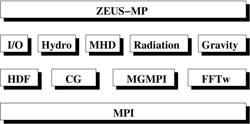
Figure 1.— Software implementation within ZEUS-MP.

Figure 1 summarizes the dependencies of ZEUS-MP’s major physics and I/O modules on underlying software libraries. The Message Passing Interface (MPI) software library is used to implement parallelism in ZEUS-MP and lies at the foundation of the code. This library is available on all NSF and DOE supercomputing facilities and may be freely downloaded for installation on small private clusters. ZEUS-MP’s linear system solvers and I/O drivers access MPI functions directly and act in service of the top layer of physics modules, which are described in the following subsections.

3.1. Hydrodynamics

Equations (1) through (5) provide the most complete physical description which may be invoked by ZEUS-MP to characterize a problem of interest. There exist classes of problems, however, for which either radiation or magnetic fields (or both) are not relevant and thus may be ignored. In such circumstances, ZEUS-MP evolves an appropriately reduced subset of field variables and solves only those equations needed to close the system. ZEUS-MP may therefore define systems of equations for pure HD, MHD, RHD, or RMHD problems as necessary. We begin the description of our numerical methods by considering purely hydrodynamic problems in this section; we introduce additional equations as we expand the discussion of physical processes.

Tracing their ancestry back to a two-dimensional, Eulerian hydrodynamics (HD) code for simulations of rotating protostellar collapse (Norman et al., 1980), all ZEUS codes are rooted in an HD algorithm based upon the method of finite differences on a staggered mesh (Norman, 1980; Norman & Winkler, 1986), which incorporates a second order-accurate, monotonic advection scheme (van Leer, 1977). The basic elements of the ZEUS scheme arise from consideration of how the evolution of a fluid element may be properly described on an adaptive mesh whose grid lines move with arbitrary velocity, ${\bf v_{g}}$. Following the analysis in Winkler et al. (1984), we identify three pertinent time derivatives in an adaptive coordinate system: (1) the Eulerian time derivative ($\partial/\partial t$), taken with respect to coordinates fixed in the laboratory frame, (2) the Lagrangean derivative ($D/Dt$; cf. equation 6), taken with respect to a definite fluid element, and (3) the adaptive-mesh derivative ($d/dt$), taken with respect to fixed values of the adaptive mesh coordinates. Identifying $dV$ as a volume element bounded by fixed values of the adaptive mesh and $d{\bf S}$ as the surface bounding this element, one may employ the formalism of Winkler et al. (1984) to split the fluid equations into two distinct solution steps: the source step, in which we solve

$$\rho{\partial{\bf v}\over\partial t} = -{\bf\nabla}{\rm p}\ -\ {\bf\nabla\cdot}{\bf Q}\ -\ {\rho{\bf\nabla}\Phi};$$ (16)

$${\partial{\rm e}\over\partial t} = -{\rm p}{\bf\nabla\cdot}{\bf v}\ -\ {\bf\nabla}{\bf v}:{\bf Q};$$ (17)

and the transport step, whence

$${d\over dt}\int_{V}\rho~{}dV = -\oint_{dV}\rho~{}({\bf v}-{\bf v_{g}})\cdot d{\bf S};$$ (18)

$${d\over dt}\int_{V}\rho{\bf v}~{}dV = -\oint_{dV}\rho{\bf v}~{}({\bf v}-{\bf v_{g}})\cdot d{\bf S};$$ (19)

$${d\over dt}\int_{V}{\rm e}~{}dV = -\oint_{dV}{\rm e}~{}({\bf v}-{\bf v_{g}})\cdot d{\bf S};$$ (20)

where ${\bf v_{g}}$ is the local grid velocity. Equations (16) and (17) have been further modified to include an artificial viscous pressure, ${\bf Q}$. ZEUS-MP employs the method due to von Neumann & Richtmyer (1950) to apply viscous pressure at shock fronts. This approach is known to provide spurious viscous heating in convergent coordinate geometries even when no material compression is present. Tscharnuter & Winkler (1979) describe a tensor formalism for artificial viscosity which avoids this problem; an implementation of this method will be provided in a future release of ZEUS-MP. For problems involving very strong shocks and stagnated flows, the artificial viscosity may be augmented with an additional term which is linear in velocity and depends upon the local sound speed. The precise forms of the quadratic and linear viscosity terms are documented in Appendix B.

3.2. MHD

The treatment of MHD waves in ZEUS-MP  is by necessity more complex than that for HD waves because MHD waves fall into two distinct families: (1) longitudinal, compressive (fast and slow magnetosonic); and (2) transverse, non-compressive (Alfvén) waves. The former family may be treated in the source-step portion of the ZEUS solution in a similar fashion to their hydrodynamic analogs, but the latter wave family couples directly to the magnetic induction equation and therefore requires a more complex treatment. From the algorithmic perspective, the inclusion of MHD into the ZEUS scheme has two consequences: (1) fluid accelerations due to compressive MHD waves introduce additional terms in equation (16); (2) fluid accelerations due to transverse MHD introduce additional velocity acceleration terms which, owing to the coupling to the induction equation, are computed in a separate step which follows the source step update but precedes the “transport” (i.e. fluid advection) update. In this way, the updates due to fluid advection are deferred until all updates to the velocities are properly recorded. As will be extensively described in this section, the fluid accelerations due to transverse MHD waves are combined with the evolution equation for ${\bf B}$ because of the tight mathematical coupling between the two solutions.

We guide the following discussion by providing, in the continuum limit, the final result. With the inclusion of MHD, the source/transport solution sequence expands to begin with an MHD-augmented “source” step:

$$\rho{\partial{\bf v}\over\partial t} = -{\bf\nabla}{\rm p}-\ {\bf\nabla}(B^{2}/8\pi)\ -\ {\bf\nabla\cdot}{\bf Q}\ -\ {\rho{\bf\nabla}\Phi};$$ (21)

$${\partial{\rm e}\over\partial t} = \ -{\rm p}{\bf\nabla\cdot}{\bf v}\ -\ {\bf\nabla}{\bf v}:{\bf Q};$$ (22)

This is followed by an MOCCT step, whence

$$\rho{\partial{\bf v}\over\partial t}\Bigg{|}_{\rm final} = \rho{\partial{\bf v}\over\partial t}\Bigg{|}_{\rm source~{}step}\ +\ {1\over 4\pi}\left({\bf B}\cdot{\bf\nabla}\right){\bf B};$$ (23)

$${d\over dt}\int_{S}{\bf B}\cdot{\bf dS} = \vec{\epsilon}\cdot{\bf dl},$$ (24)

where $\vec{\epsilon}$ is the electromotive force (EMF) and is given by

$$\vec{\epsilon}\ =\ ({\bf v}-{\bf v_{g}}){\bf\times}{\bf B}.$$ (25)

With velocities and ${\bf B}$ fields fully updated, we then proceed to the “transport” step as written in equations (18) through (20).

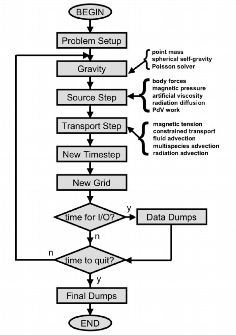
Figure 2.— Program control for ZEUS-MP.

Figure 2 shows the program control logic used to implement the solution outlined by equations (21)-(24) and the previously-written expressions (18)-(20). Once the problem has been initialized, Poisson’s equation is solved to compute the gravitational potential. In the source step, updates due to longitudinal forces (thermal and magnetic), radiation stress, artificial viscosity, energy exchange between the gas and radiation field, and pdV work are performed at fixed values of the coordinates. Accelerations due to transverse MHD waves are then computed and magnetic field components are updated. Finally, velocities updated via (21) and (23) are used to advect field variables through the moving mesh in the transport step. Advection is performed in a series of directional sweeps which are cyclically permuted at each time step.

The remainder of this section serves to derive the new expressions appearing in (21), (23), and (24), and to document their solution. We begin by first considering the Lorentz acceleration term in the gas momentum equation (2). Using the vector identity

$$\left({\bf\nabla\times}{\bf B}\right){\bf\times}{\bf B}=-{\bf\nabla}\left(B^{2}/2\right)\ +\ \left({\bf B}\cdot{\bf\nabla}\right){\bf B}$$ (26)

we expand the Lorentz acceleration term such that (2) becomes (ignoring radiation)

$$\rho{D{\bf v}\over Dt} = -{\bf\nabla}{\rm p}\ -\ {\bf\nabla}(B^{2}/8\pi)\ +\ {1\over 4\pi}\left({\bf B}\cdot{\bf\nabla}\right){\bf B}$$ (27)

$$- {\rho{\bf\nabla}\Phi}.$$

The second term on the RHS of (27) is the gradient of the magnetic pressure. This term, which provides the contribution from the compressive magnetosonic waves, is clearly a longitudinal force and is differenced in space and time identically to the thermal pressure term. This expression is thus evaluated simultaneously with the other contributions to the “source step” portion of the momentum equation (equation 21); contributions from the magnetic pressure to the discrete representation of (21) along each axis are shown in equations (B10) through (B12), with notational definitions provided by expressions (B19) through (B30), in appendix B.

The third term on the RHS of (27) represents magnetic tension in curved field lines and is transverse to the gradient of ${\bf B}$. This term, which is added to the solution sequence as equation (23) couples to the magnetic induction equation to produce Alfvén waves; the magnetic tension force and the induction equation (5) are therefore solved by a single procedure: the Method of Characteristics + Constrained Transport (MOCCT).

ZEUS-MP employs the MOCCT method of  Hawley & Stone (1995), which is a generalization of the algorithm described in  Stone & Norman (1992b) to 3D, with some slight modifications that improve numerical stability. To describe MOCCT, we first derive the moving frame induction equation. Recall that equation (5) is derived from Faraday’s law

$${\partial{\bf B}\over\partial t}\ =\ -c{\bf\nabla\times}{\bf E},$$ (28)

where ${\bf E}$, ${\bf B}$ and the time derivative are measured in the Eulerian frame. The electric field ${\bf E}$ is specified from Ohm’s law

$$c{\bf E}=-{\bf v}{\bf\times}{\bf B}+{\bf J}/\sigma.$$ (29)

Equation (5) results when we substitute equation 29 into equation 28, and let the conductivity $\sigma\rightarrow\infty$. Integrating equation 28 over a moving surface element $S(t)$ bounded by a moving circuit $C(t)$, the general form of Faraday’s law is

$${d\over dt}\int_{S}{\bf B}\cdot{\bf dS}=-c\oint_{C}{\bf E}^{\prime}\cdot{\bf dl}$$ (30)

where ${\bf E}^{\prime}$ is the electric field measured in the moving frame. To first order in $v/c$, ${\bf E}^{\prime}={\bf E}+({\bf v_{g}}{\bf\times}{\bf B})/c$. From equation 29, for a perfectly conducting fluid ${\bf E}=-{\bf v}{\bf\times}{\bf B}/c$. Combining these two results and substituting into equation 30, we get

$${d\over dt}\int_{S}{\bf B}\cdot{\bf dS}=\oint_{C}({\bf v}-{\bf v_{g}}){\bf\times}{\bf B}\cdot{\bf dl}.$$ (31)

Equation (31) states that the time rate of change of the magnetic flux piercing $S$

$$\phi_{S}=\int_{S}{\bf B}\cdot{\bf dS}$$ (32)

is given by the line integral of the electromotive force (EMF) $\mathbf{\epsilon=(v-v_{g}){\bf\times}B}$ along $C$:

$${d\phi_{S}\over dt}=\oint_{C}{\epsilon}\cdot{\bf dl}.$$ (33)

Equation (33), using (32), is equivalent to expression (24) appearing in our grand solution outline, and it forms, along with equation (23), the target for our MOCCT algorithm. Equation (33) is familiar from standard texts on electrodynamics, only now $S$ and $C$ are moving with respect to the Eulerian frame. If ${\bf v_{g}}={\bf v}$, we recover the well known flux-freezing result, $d\phi_{S}/dt=D\phi_{S}/Dt=0.$

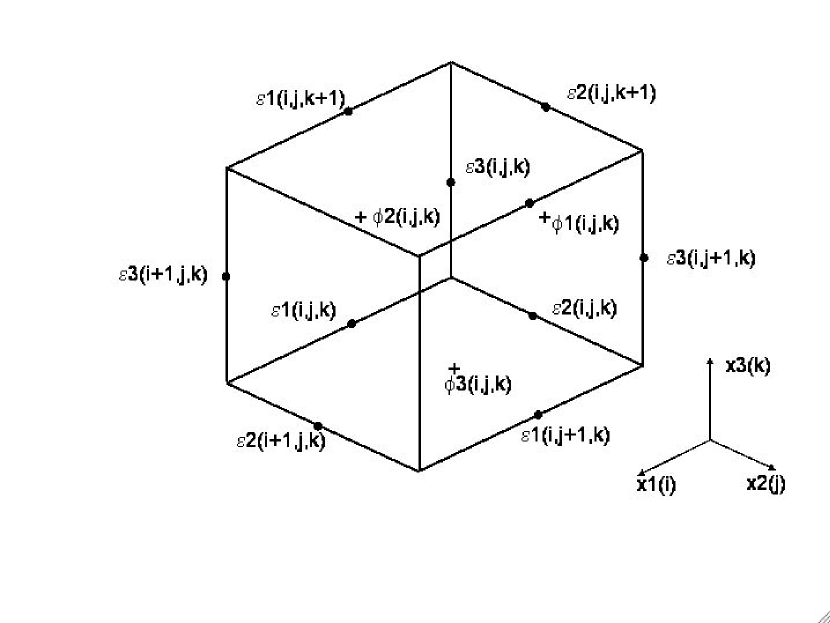
Figure 3.— Centering of magnetic field variables in ZEUS-MP.

As discussed in Evans & Hawley (1988); Stone & Norman (1992b); Hawley & Stone (1995), equation (33) is in the form which guarantees divergence-free magnetic field transport when finite differenced, provided the EMFs are evaluated once and only once per time step. Referring to the unit cell shown in Figure 3, we can write the discrete form of equation (33) as

$${{\phi 1_{i,j,k}^{n+1}-\phi 1_{i,j,k}^{n}}\over{\Delta t}} = \epsilon 2_{i,j,k}\Delta x2_{i,j}+\epsilon 3_{i,j+1,k}\Delta x3_{i,j+1,k}$$ (34)

$$- \epsilon 2_{i,j,k+1}\Delta x2_{i,j}-\epsilon 3_{i,j,k}\Delta x3_{i,j,k};$$

$${{\phi 2_{i,j,k}^{n+1}-\phi 2_{i,j,k}^{n}}\over{\Delta t}} = \epsilon 1_{i,j,k+1}\Delta x1_{i}+\epsilon 3_{i,j+1,k}\Delta x3_{i,j,k}$$ (35)

$$- \epsilon 1_{i,j,k}\Delta x1_{i}-\epsilon 3_{i+1,j,k}\Delta x3_{i+1,j,k};$$

$${{\phi 3_{i,j,k}^{n+1}-\phi 3_{i,j,k}^{n}}\over{\Delta t}} = \epsilon 1_{i,j,k}\Delta x1_{i}+\epsilon 2_{i+1,j,k}\Delta x2_{i+1,j}$$ (36)

$$- \epsilon 1_{i,j+1,k}\Delta x1_{i}-\epsilon 2_{i,j,k}\Delta x2_{i,j},$$

where $\phi 1,\phi 2,\phi 3$ are the face-centered magnetic fluxes piercing the cell faces whose unit normals are in the $\bf{n_{1},n_{2},n_{3}}$ directions, respectively, $\epsilon 1,\epsilon 2,\epsilon 3$ are components of the edge-centered EMFs, and $\Delta x1,\Delta x2,\Delta x3$ are the coordinate distances of the cell edges. The peculiar subscripting of these line elements is made clear in Appendix C. It is easy to see that for any choice of EMFs, ${\bf B}^{n+1}$ will be divergence-free provided ${\bf B}^{n}$ is divergence-free. By Gauss’s theorem, $\int_{V}{\bf\nabla\cdot}{\bf B}dV=\oint_{S}{\bf B}\cdot{\bf dS}=0$, where the second equality follows from the fact ${\bf\nabla\cdot}{\bf B}=0.$ Analytically, the time derivative of ${\bf\nabla\cdot}{\bf B}$ is also zero. Numerically,

$${d\over dt}\int_{V}{\bf\nabla\cdot}{\bf B}dV = {d\over dt}\oint_{S}{\bf B}\cdot{\bf dS}\approx\sum_{faces=1}^{6}d\phi/dt$$ (37)

$$= \sum_{faces=1}^{6}\sum_{edges=1}^{4}\epsilon\cdot{\bf dl}=0.$$

The last equality results from the fact that when summing over all the faces and edges of a cell, each EMF appears twice with a change of sign, and thus cancel in pairs.

In principle, one could use any method to compute the EMF within the CT formalism and still maintain divergence-free fields. In practice, a method must be used which stably and accurately propagates both MHD wave types: longitudinal, compressive (fast and slow magnetosonic) waves, and the transverse, non-compressive (Alfvén) waves. As noted previously, the first wave type is straightforwardly incorporated into the treatment of the compressive hydrodynamic waves; the real difficulty arises in the treatment of the Alfvén waves.

In ideal MHD, Alfvén waves can exhibit discontinuities (rotational, transverse) at current sheets. Unlike hydrodynamical shocks, these structures are not dissipative, which rules out the use of dissipative numerical algorithms to model them. In addition, Alfvén waves tightly couple the evolution equations for the velocity and magnetic field components perpendicular to the direction of propagation. This rules out operator operator splitting these components. Finally, we need an algorithm that can be combined with CT to give both divergence-free transport of fields and correct local dynamics. This will be achieved if the EMFs used in the CT scheme contain information about all wave modes, which for stability, must be appropriately upwinded. These multiple requirements can be met using the Method of Characteristics (MOC) to compute the EMFs. The resulting hybrid scheme is MOCCT (Stone & Norman, 1992b; Hawley & Stone, 1995).

Schematically, the EMFs can be written as (ignoring ${\bf v_{g}}$ for simplicity)

$$\epsilon 1_{i,j,k}\ =\ v2^{*}_{i,j,k}~{}b3^{*}_{i,j,k}\ -\ v3^{*}_{i,j,k}~{}b2^{*}_{i,j,k}$$ (38)

$$\epsilon 2_{i,j,k}\ =\ v3^{*}_{i,j,k}~{}b1^{*}_{i,j,k}\ -\ v1^{*}_{i,j,k}~{}b3^{*}_{i,j,k}$$ (39)

$$\epsilon 3_{i,j,k}\ =\ v1^{*}_{i,j,k}~{}b2^{*}_{i,j,k}\ -\ v2^{*}_{i,j,k}~{}b1^{*}_{i,j,k}$$ (40)

where the starred quantities represent time-centered values for these variables resulting from the solution of the characteristic equations at the centers of zone edges where the EMFs are located. To simplify, we apply MOC to the Alfvén waves only, as the longitudinal modes are adequately handled in a previous step by finite difference methods.

Because the MOC is applied only to transverse waves, we may derive the appropriate differential equations by considering the 1-D MHD wave equations for an incompressible fluid (Stone & Norman, 1992b) which reduce to

$${\partial v\over\partial t}=\frac{B_{x}}{\rho}{\partial B\over\partial x}-{\partial\over\partial x}(v_{x}v),$$ (41)

$${\partial B\over\partial t}=B_{x}{\partial v\over\partial x}-{\partial\over\partial x}(v_{x}B),$$ (42)

where we have used the divergence-free constraint in one dimension (which implies $\partial B_{x}/\partial x\equiv 0)$ and the non-compressive nature of Alfvén waves (which implies $\partial v_{x}/\partial x\equiv 0)$.

We can rewrite the coupled equations (41) and (42) in characteristic form by multiplying equation (42) by $\rho^{-1/2}$ and then adding and subtracting them, yielding

$${\mathcal{D}v\over\mathcal{D}t}\pm\frac{1}{\rho^{1/2}}{\mathcal{D}B\over\mathcal{D}t}=0.$$ (43)

The plus sign denotes the characteristic equation along the forward facing characteristic $C^{+}$, while the minus sign denotes the characteristic equation along the backward facing characteristic $C^{-}$. The comoving derivative used in equation (43) is defined as

$$\mathcal{D}/\mathcal{D}t\equiv\partial/\partial t+(v_{x}\mp B_{x}/\rho^{1/2})\partial/\partial x,$$ (44)

where the minus (plus) sign is taken for the comoving derivative along the $C^{+}(C^{-})$ characteristic. Note that the coefficient of the second term in equation (44) is just the Alfvén velocity in the moving fluid, $v_{x}\pm v_{A}$. Physically, equations (43) state that along characteristics, which are straight lines in spacetime with slopes $v_{x}\pm v_{A}$, the changes in the velocity and magnetic field components in each direction are not independent.

The finite-difference equations used to solve the characteristic equations (43) can be generated as follows. Consider the one dimensional space-time diagram centered at the position of one of twelve edge-centered EMFs where we require the values $v_{i}^{*},B_{i}^{*}$ (see Figure 5). Extrapolating back in time along the characteristics $C^{+}$ and $C^{-}$ to time level $n$ defines the “footpoints”. By using upwind van Leer (1977) interpolation, we can compute the time-averaged values for these variables in each domain of dependence. For both the velocities and the magnetic fields the characteristic speed $v_{x}\pm v_{A}$ are used to compute the footpoint values $v_{i}^{+,n},B_{i}^{+,n},v_{i}^{-,n},B_{i}^{-,n}$. The finite difference equations along $C^{+}$ and $C^{-}$ become

$$(v_{i}^{*}-v_{i}^{+,n})+(B_{i}^{*}-B_{i}^{+,n})/(\rho_{i}^{+})^{1/2}=0,$$ (45)

$$(v_{i}^{*}-v_{i}^{-,n})-(B_{i}^{*}-B_{i}^{-,n})/(\rho_{i}^{-})^{1/2}=0,$$ (46)

where the subscript $i$ refers to cell $i$, not the $i$-th component of the vectors ${\bf v},{\bf B}$. For simplicity, we set $\rho_{i}^{+}=\rho_{i-1}^{n}$ and $\rho_{i}^{-}=\rho_{i}^{n}$. The two linear equations for the two unknowns $v_{i}^{*}$ and $B_{i}^{*}$ are then solved algebraically.

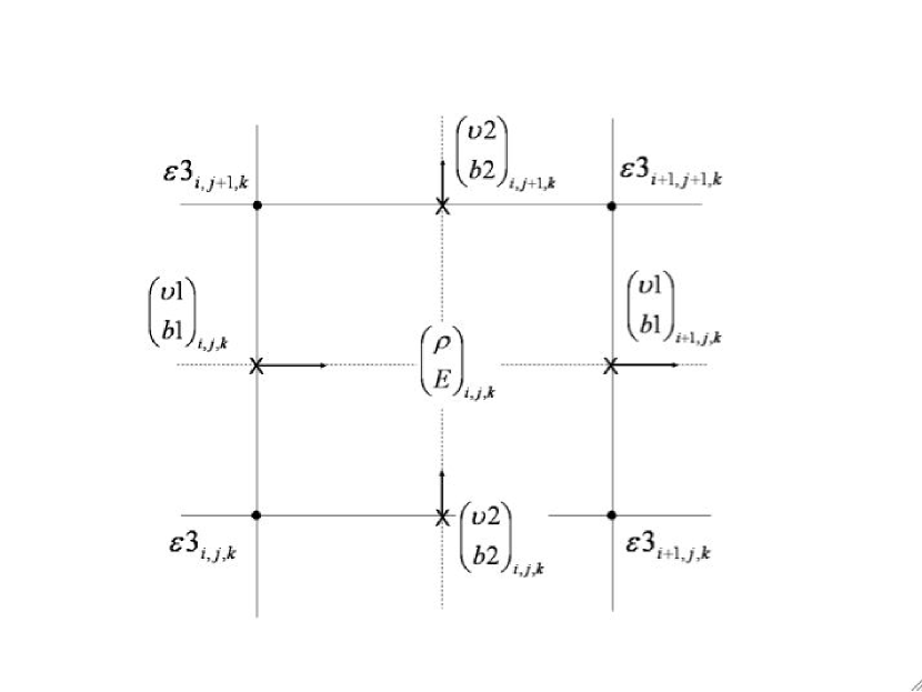
Figure 4.— A two dimensional ($x1-x2$) slice through the unit cell in Figure 3 containing the four $\epsilon 3$’s. The computation of $\epsilon 3_{i,j,k}$ is illustrated in Figure 5.

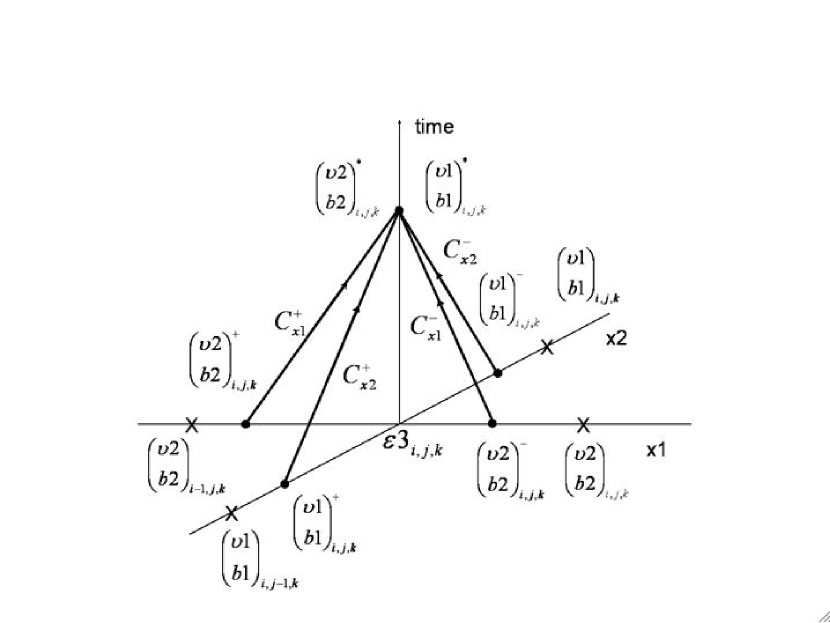
Figure 5.— The computation of $\epsilon 3_{i,j,k}$ involves the solution of two 1-D characteristic equations for Alfvén waves confined to the ($x1-x2$) plane. The space-time diagrams for the solution of $b2^{*},v2^{*}$ due to Alfvén waves propagating parallel to the $x1$ axis, and for the solution of $b1^{*},v1^{*}$ due to Alfvén waves propagating parallel to the $x2$ axis are displayed.

For our multidimensional calculations, the characteristic equations are solved in a directionally split fashion on planes passing through the center of the cell and the cell edges where the EMFs are to be evaluated. To illustrate, consider the calculation of $\epsilon 3_{i,j,k}$ (Eq. 40). The plane parallel to the $x1-x2$ plane passing through the four $\epsilon 3$’s in Figure 3 is shown in Figure 4. Evaluating $\epsilon 3_{i,j,k}$ requires values for $b1^{*},v1^{*},b2^{*},$ and $v2^{*}$ at the cell corner $(x1_{i},x2_{j},x3_{k})$. First, as outlined above, one computes $b2^{*},v2^{*}$ by solving the characteristic equations for Alfvén waves propagating in the $x1$ direction (Figure 5). When calculating the location of the footpoints, $v1$ and the Alfvén speed are averaged to the zone corner. Then, the procedure is repeated for $b1^{*},v1^{*}$ by solving the characteristic equations for Alfvén waves propagating in the $x2$ direction, using $v2$ and the Alfvén speed averaged to the zone corner. Once all the $\epsilon 3$’s are evaluated in this way, the analogous procedure is followed for slices containing $\epsilon 1$ and $\epsilon 2$. Only after all the EMFs have been evaluated over the entire grid can the induction equation equation be updated in a divergence-free fashion.

Finally, we consider how the fluid momentum is updated due to the Lorentz Force. The key point is that we do not want to throw away the fluid accelerations arising from Alfvén waves that are implicit in the solution to the characteristic equations (45) and (46). For example, the acceleration of $v3$ by the transverse magnetic forces is given by

$$\rho{\partial v_{3}\over\partial t}=-{\bf\nabla}_{(3)}(B^{2}/8\pi)+\frac{1}{4\pi}({\bf B}\cdot{\bf\nabla})B_{3},$$ (47)

or in terms of the EMFs:

$$\rho_{i,j,k}(\frac{v3_{i,j,k}^{n+1}-v3_{i,j,k}^{n}}{\Delta t}) = \frac{1}{4\pi}[\overline{b1}(\frac{b3^{*}_{\epsilon 2(i+1,j,k)}-b3^{*}_{\epsilon 2(i,j,k)}}{\Delta x1})$$ (48)

$$+ \overline{b2}(\frac{b3^{*}_{\epsilon 1(i,j+1,k)}-b3^{*}_{\epsilon 1(i,j,k)}}{\Delta x2})]$$

where $\overline{b1}$ and $\overline{b2}$ are four-point averages of the magnetic field to the spatial location of $v3$, and the $b3^{*}$’s are those values that enter into the EMF’s referred to in the subscripts (see Figure 3.) Similarly, the magnetic pressure calculation is

$$\rho_{i,j,k}(\frac{v3_{i,j,k}^{n+1}-v3_{i,j,k}^{n}}{\Delta t})=-\frac{1}{4\pi}[\overline{b1}(\frac{\Delta b1}{\Delta x3})+\overline{b2}(\frac{\Delta b2}{\Delta x3})].$$ (49)

The evaluation of the EMF’s outlined by equations (38) through (40) has been modified according to a prescription due to Hawley & Stone (1995), in which each of the two $vB$ product terms is computed from a mix of quantities computed directly from the characteristic equations with quantities estimated from simple advection. Full details are provided in Appendix C, but the idea may illustrated by an appropriate rewrite of (40) for the evaluation of $\epsilon 3_{i,j,k}$:

$$\epsilon 3_{i,j,k} = 0.5*\left(v1^{*}_{i,j,k}~{}\overline{b2}_{i,j,k}+\overline{v1}_{i,j,k}~{}b2^{*}_{i,j,k}\right)$$ (50)

$$- 0.5*\left(v2^{*}_{i,j,k}~{}\overline{b1}_{i,j,k}+\overline{v2}_{i,j,k}~{}b1^{*}_{i,j,k}\right),$$

where the starred quantities are derived from characteristic solutions and the barred quantities arise from upwinded averages along the appropriate fluid velocity component. This modification (which engenders the “HS” in “HSMOCCT”) introduces a measure of diffusivity into the propagation of Alfvén waves which is not present in the MOC scheme described in Stone & Norman (1992b). Hawley & Stone (1995) note that this change resulted in a more robust algorithm when applied to fully multidimensional problems characterized by strong magnetic discontinuities.

3.3. Radiation Diffusion

The inclusion of radiation in the system of fluid equations to be solved introduces four changes in the numerical solution. First, an additional contribution to the source-step momentum equation arises from the radiation flux:

$$\rho{\partial{\bf v}\over\partial t}\ =\ -{\bf\nabla}{\rm p}\ -\ {\bf\nabla\cdot}{\bf Q}\ +\ \left(\chi\over c\right){\bf F}\ -\ {\rho{\bf\nabla}\Phi};.$$ (51)

Second, new source/sink terms appear in the source-step gas energy equation:

$${\partial{\rm e}\over\partial t}\ =\ c{\kappa_{\rm E}}{\rm E}\ -4\pi{\kappa_{\rm P}}{\rm B_{p}}\ -{\rm p}{\bf\nabla\cdot}{\bf v}\ -\ {\bf\nabla}{\bf v}:{\bf Q}.$$ (52)

Third, a new source-step equation is added for the radiation energy density:

$${\partial{\rm E}\over\partial t}\ =\ 4\pi{\kappa_{\rm P}}{\rm B_{p}}\ -\ c{\kappa_{\rm E}}{\rm E}\ -\ {\bf\nabla\cdot}{\bf F}-{\bf\nabla}{\bf v}:{\bf P};$$ (53)

and fourth, an additional advection equation for ${\rm E}$ is added to the transport step:

$${d\over dt}\int_{V}{\rm E}~{}dV\ =\ -\oint_{dV}{\rm E}~{}({\bf v}-{\bf v_{g}})\cdot d{\bf S}.$$ (54)

In comparing equations (51) - (53) with either the pure HD equations (16) - (17) or the MHD analogs (21) - (24), it is clear that the inclusion of radiation physics may be made to the HD or MHD systems of equations with equal ease. Similary, the transport step is augmented with a solution of (54) in either scenario.

ZEUS-MP computes the evolution of radiating fluid flows through an implicit solution to the coupled gas and radiation energy equations (52) and (53). Rather than solve the time-dependent radiation momentum equation and treat the flux, ${\bf F}$, as an additional dependent variable, we adopt the flux-limited diffusion (FLD) approximation as shown in (11). This allows an algebraic substitution for ${\bf F}$ in the flux-divergence term of the source-step equation (53) for E and avoids the need for an additional advection equation for the flux. The FLD approximation is an attractive choice for multidimensional RHD applications for which local heating/cooling approximations are inadequate. With regard to computational expense, FLD offers enormous economy relative to exact Boltzmann solutions for the photon distribution function because the dimensionality of the problem is reduced by 2 when the angular variation of the radiation field is integrated away. Additionally, the mathematical structure of the FLD equations makes the solution amenable to parallel implementation. Fundamentally, however, the flux-limiter is a mathematical construction which interpolates between the limiting cases of transparency and extreme opacity in a manner that (hopefully) retains sufficient accuracy in the more difficult semi-transparent regime. Precisely what constitutes “sufficient accuracy” is dictated by the needs of the particular application, and the techniques for meeting that requirement may likewise depend upon the research problem. Levermore & Pomraning (1981) (LP) constructed an FLD theory which derived a form of $\Lambda_{\rm E}$ widely adopted in astrophysical applications (and in this paper). In their work, LP use simple test problems to check the accuracy of their FLD solution against exact transport solutions. In simulations of core-collapse supernovae, Liebendörfer et al. (2004) compared calculations employing energy-dependent multi-group FLD (MGFLD) calculations against those run with an exact Boltzmann solver and found alternate forms of the limiter which better treated the transport through the semi-transparent shocked material in the post-bounce environment. These calculations and others have shown that FLD or MGFLD techniques can yield solutions that compare favorably with exact transport, but that a “one size fits all” prescription for the flux limiter is not to be expected.

In the context of applications, two other vulnerabilities of FLD bear consideration. Hayes & Norman (2003) have compared FLD to VTEF solutions in problems characterized by highly anisotropic radiation fields. Because the FLD equation for flux is a function of the local gradient in E, radiation tends to flow in the direction of radiation energy gradients even when such behavior is not physically expected, as in cases where radiation from a distant source is shadowed by an opaque object. In applications where the directional dependence of the radiation is relevant (Turner et al. (2005) discuss a possible example), an FLD prescription may be of limited reliability. A second vulnerability concerns numerical resolution. As discussed in detail by Mihalas & Mihalas (1984), the diffusion equation must be flux-limited because numerically, the discrete diffusion equation advances a radiation wave one mean-free path ($\lambda$) per time step. Flux limiters are designed to act when $\lambda/\Delta t$ exceeds c, which ordinarily one expects in a transparent medium. A problem can arise in extremely opaque media however, when the physical mean-free path is much smaller than the width of a grid cell. In this case, $\lambda$ is unresolved, and the effective propagation length scale is now determined by the much larger zone size. Because the signal speed is much less than c, the flux-limiter provides no constraint on the propagation of radiation. This can lead to unphysically rapid heating of irradiated boundary layers which are spatially unresolved. This problem has long bedeviled terrestrial transport applications; whether this represents a liability for a given astrophysical application should be carefully assessed by the user.

We consider now some basic details of our FLD module. In our RHD prescription, matter and radiation may exchange energy through absorption and emission processes represented by the right-hand sides of equations (3) and (4), and the radiation stress term on the LHS of (4). The radiation energy budget is further influenced by spatial transport, which we treat with the diffusion operator. The high radiation signal speed in transparent media mandates an implicit solution to the radiation energy equation. Coupling between the radiation and matter is treated via an iterative scheme based upon Newton’s method. Recently, Turner & Stone (2001) published a new FLD module for the ZEUS-2D code. The physical assumptions underlying their method are consistent with those identified here, but the mathematical treatment for solving the coupled system differs from what we describe below.

Our construction of a linear system for the 3-D RHD equations begins with expressions for the spatially and temporally discretized gas and radiation energy equations. Consider the gas and radiation energy densities to be defined at discrete points along 3 orthogonal axes denoted by $i$, $j$, and $k$; i.e. ${\rm e}\rightarrow{\rm e}_{i,j,k}$ and ${\rm E}\rightarrow{\rm E}_{i,j,k}$. We approximate the partial time derivative in terms of a time-centered difference between two adjacent time levels, $t^{n}$ and $t^{n+1}$: ${\Delta t}\equiv t^{n+1}-t^{n}$. We then define two functions in ${\rm e}_{i,j,k}$ and ${\rm E}_{i,j,k}$:

$$f^{(1)}_{i,j,k} = {\rm E}^{n+1}_{i,j,k}\ -\ {\rm E}^{n}_{i,j,k}$$ (55)

$$- {\Delta t}\left[4\pi{\kappa_{\rm P}}{\rm B_{p}}-c{\kappa_{\rm E}}{\rm E}^{n+1}_{i,j,k}\right]$$

$$- {\Delta t}\left[{\bf\nabla\cdot}{\bf F}_{i,j,k}^{n+1}+{\bf\nabla}{\bf v}:{\bf P}_{i,j,k}^{n+1}\right];$$

$$f^{(2)}_{i,j,k} = {\rm e}^{n+1}_{i,j,k}\ -\ {\rm e}^{n}_{i,j,k}$$ (56)

$$- {\Delta t}\left[-4\pi{\kappa_{\rm P}}{\rm B_{p}}+c{\kappa_{\rm E}}{\rm E}^{n+1}_{i,j,k}\right]$$

$$+ {\Delta t}{\rm p}{\bf\nabla\cdot}{\bf v}.$$

For notational economy, we have confined explicit reference to coordinate indices and time level to the gas and radiation energy variables. As written above, the functions $f^{(1)}_{i,j,k}$ and $f^{(2)}_{i,j,k}$ are identically zero for a consistent solution for ${\rm e}_{i,j,k}$ and ${\rm E}_{i,j,k}$. We employ a Newton-Raphson iteration scheme to find the roots of (56) and (55). To construct a discrete system of equations which is linear in both energy variables, we evaluate the E-dependent flux limiter from values of E at the previous time level n. The thermal pressure, Planck functions, and opacities are updated at each iteration. The velocities are roughly (but not formally) time-centered, having been updated with contributions from body forces and artificial viscosity prior to the radiation solution (cf. figure 2). We may write the linear system to be solved as

$$J\left(x\right)\delta x\ =\ -f\left(x\right).$$ (57)

In (57), $x$ is the vector of gas and radiation energy variables: $x\equiv\left({\rm E}_{i,j,k},{\rm e}_{i,j,k}\right)$. Likewise, the solution vector $\delta x$ is the set of corrections to these variables, $\left(\delta{\rm E}_{i,j,k},\delta{\rm e}_{i,j,k}\right)$. $f$ represents the vector of discrete functions $\left(f^{(1)}_{i,j,k},f^{(2)}_{i,j,k}\right)$, and $J\left(x\right)$ is the Jacobian, $\partial f^{i}/\partial x^{j}$.

As written above, expression (57) represents a matrix of size (2N)x(2N), where N is the product of the numbers of mesh points along each coordinate axis. As will be shown in appendix D the corrections, $\delta{\rm e}_{i,j,k}$, to the gas energies may be analytically expressed as functions of the radiation energy corrections, $\delta{\rm E}_{i,j,k}$. This allows the solution of a reduced system of size NxN for the vector of $\delta{\rm E}_{i,j,k}$, from which the set of $\delta{\rm e}_{i,j,k}$ are immediately obtained. These corrections are used to iteratively update the trial values of ${\rm e}_{i,j,k}$ and ${\rm E}_{i,j,k}$. We have found in a variety of test problems that typically 2 to 10 N-R iterations are required for a converged solution at each time step.

Each iteration in the N-R loop involves a linear system which must be solved with matrix algebra. Our solution for Poisson’s equation also requires a linear system solver. We discuss the types of linear solvers implemented in ZEUS-MP separately in §3.8, with additional details provided in appendices D, E, and F.

3.4. Self Gravity

ZEUS-MP treats Newtonian gravity at three different levels of approximation: (1) point-mass potentials, (2) spherically-symmetric gravity (${\bf\nabla}\Phi=GM/r^{2}$), and (3) exact solutions to Poisson’s equation (15). The first two options are trivial to implement; in this discussion we therefore focus on the final option. In three dimensions, the discrete Laplacian operator connects a mesh point at coordinate (i,j,k) with both adjacent neighbors along each axis; thus a finite-differenced form of (15) takes the following form:

$$a_{1}\Phi_{i,j,k-1}\ +\ a_{2}\Phi_{i,j-1,k}\ +\ a_{3}\Phi_{i-1,j,k} +$$

$$a_{4}\Phi_{i+1,j,k}\ +\ a_{5}\Phi_{i,j+1,k}\ +\ a_{6}\Phi_{i,j,k+1} +$$

$$a_{7}\Phi_{i,j,k} = 4\pi G\rho_{i,j,k}.$$ (58)

If (58) is defined on a Cartesian mesh in which the zone spacing along each axis is uniform, then the “$a$” coefficients in equation 58 are constant over the problem domain. If, in addition to uniform gridding, the problem data is characterized by spatial periodicity, then Fast Fourier Transform (FFT) algorithms offer a highly efficient method for solving (58). For this class of problems (see Li et al. (2004) for a recent example), ZEUS-MP provides an FFT module based upon the publicly available “FFTw” software (Frigo & Johnson, 2005). While FFT-based methods are not in general restricted only to periodic problems, we emphasize that the module implemented in ZEUS-MP is valid only for 3-D problems on uniform Cartesian meshes with triply-periodic boundaries.

For multidimensional problems which do not meet all of the validity criteria for the FFTw solver, ZEUS-MP provides two additional solution modules. The most general of these accommodates 2-D and 3-D grids in Cartesian, cylindrical, and spherical geometries and is based upon the same CG solver provided for the FLD radiation equations. A second module currently written for 3-D Cartesian meshes with Dirichlet or Neumann boundary conditions is based upon the multigrid (MG) method (cf. §3.8.2).

When equation (58) is formulated as a function of ZEUS covariant grid variables, the matrix elements represented by the “$a$” coefficients take on a much more complicated functional form than the constant values which obtain for a uniform Cartesian mesh. The form of (58) written for the general class of 3-D covariant grids is documented in appendix E. Details of all three solution techniques for Poisson’s equation are written in §3.8.

3.5. Multi-species Advection

Prior public versions of ZEUS codes have treated the gas as a single species fluid. In order to be forward-compatible with physical processes such as chemistry, nuclear reactions, or lepton transport, ZEUS-MP  offers a straightforward mechanism for identifying and tracking separate chemical or nuclear species in a multi-species fluid mixture. Because ZEUS-MP solves one set of fluid equations for the total mass density, $\rho$, we have no facility for modeling phenomena in which different species possess different momentum distributions and thus move with respect to one another. Nonetheless, a wide variety of astrophysical applications are enabled with a mechanism for quantifying the abundances of separate components in a mixed fluid. Our multi-species treatment considers only the physical advection of different species across the coordinate mesh; physics modules which compute the local evolution of species concentrations (such as a nuclear burning network) must be provided by the user.

Our implementation of multispecies advection proceeds by defining a concentration array, X_n, such that $\rho{\rm X_{n}}$ is the fractional mass density of species n. The advection equations in the ZEUS transport step therefore include:

$${d\over dt}\int_{V}\left(\rho{\rm X_{n}}\right)~{}dV\ =\ -\oint_{dV}\left(\rho{\rm X_{n}}\right)~{}({\bf v}-{\bf v_{g}})\cdot d{\bf S}.$$ (59)

This construction is evaluated such that the mass fluxes used to advect individual species across the mesh lines are consistent with those used to advect the other field variables defined in the application. Discrete formulae for the conservative advection of X_n and the other hydrodynamic field variables are provided in appendix B.

3.6. Time Step Control

Maintainence of stability and accuracy in a numerical calculation requires proper management of time step evolution. The general expression regulating the time step in ZEUS-MP is written

$${\Delta t}_{\rm new} = C_{\rm cfl}$$

$$\times \left\{{1\over{\Delta t}_{\rm cs}^{2}}+{1\over{\Delta t}_{v1}^{2}}+{1\over{\Delta t}_{v2}^{2}}+{1\over{\Delta t}_{v3}^{2}}+\right.$$

$$\mbox{}\left.{1\over{\Delta t}_{\rm al}^{2}}+{1\over{\Delta t}_{\rm av}^{2}}+{1\over{\Delta t}_{\rm rd}^{2}}\right\}^{1/2},$$

in which C_cfl is the Courant factor and the ${\Delta t}^{2}$ terms are squares of the minimum values of the following quantities:

$${\Delta t}^{2}_{\rm cs} = \gamma\left(\gamma-1\right)\cdot\left({\rm e}/\rho\right)~{}/~{}\left(\Delta X_{\rm min}\right)^{2};$$ (61)

$${\Delta t}^{2}_{v1} = \left[\left(v1-vg1\right)~{}/~{}dx1a\right]^{2};$$ (62)

$${\Delta t}^{2}_{v2} = \left[\left(v2-vg2\right)~{}/~{}(g2b~{}dx2a)\right]^{2};$$ (63)

$${\Delta t}^{2}_{v3} = \left[\left(v3-vg3\right)~{}/~{}(g31b~{}g32b~{}dx3a)\right]^{2};$$ (64)

$${\Delta t}^{2}_{\rm al} = \left(\overline{b1}^{2}+\overline{b2}^{2}+\overline{b3}^{2}\right)~{}/~{}\left[4\rho\left(\Delta X\right)^{2}\right];$$ (65)

$${\Delta t}^{2}_{\rm av} = \left[4~{}{\rm qcon}~{}\left|dv\over dx\right|_{\rm max}\right]^{-2};$$ (66)

$${\Delta t}^{2}_{\rm rd} = \left[{\bf ertol}\left|{\rm E}\over{\Delta{\rm E}}\right|\right]^{2}$$ (67)

These values represent, respectively, the local sound-crossing time, the local fluid crossing time along each coordinate, the local Alfvén wave crossing time, the local viscous timescale, and a radiation timescale determined by dividing the value of ${\rm E}$ returned from the FLD solver by the time rate of change in ${\rm E}$ determined by comparing the new ${\rm E}$ to that from the previous time step. ertol is a specified tolerance which retrodictively limits the maximum fractional change in ${\rm E}$ allowed in a timestep. $\Delta X_{\rm min}$ represents the minimum length of a 3-D zone edge, i.e. MIN$\left[dx1a,~{}g2b~{}dx2a,~{}g31b~{}g32b~{}dx3a\right]$, where each zone length is expressed in terms of the local covariant grid coefficients (cf. appendix B). As expressed in (3.6), $dt_{\rm new}$ represents a trial value of the new time step, which is allowed to exceed the previous value of the time step by no more than a preset factor; i.e. ${\Delta t}_{\rm final}~{}=~{}{\rm min}\left[{\Delta t}_{\rm new},{\rm fac}\times{\Delta t}_{\rm old}\right]$, with “fac” typically equaling 1.26. This value allows the time step to increase by up to a factor of 10 every 10 cycles.

3.7. Parallelism

The most powerful computers available today are parallel systems with hundreds to thousands of processors connected into a cluster. While some systems offer a shared-memory view to the applications programmer, others, such as Beowulf clusters, do not. Thus, to maximize portability we have assumed “shared nothing” and implemented ZEUS-MP as an SPMD (Single Program, Multiple Data) parallel code using the MPI message-passing library to accomplish interprocessor communication. In this model, parallelism is affected via domain decomposition (Foster, 1995), in which each CPU stores data for and performs operations upon a unique sub-block of the problem domain. Because finite-difference forms of gradient, divergence, and Laplacian operators couple data at multiple mesh points, data must be exchanged between neighboring processors when such operations are performed along processor data boundaries. ZEUS-MP employs “asynchronous” or “non-blocking” communication functions which allow interprocessor data exchange to proceed simultaneously with computational operations. This approach provides the attractive ability to hide a large portion of the communication costs and thus improve parallel scalability. Details of our method for overlapping communication and computation operations in ZEUS-MP are provided in appendix F.

3.8. Linear Solvers

Our implicit formulation of the RHD equations and our solution to Poisson’s equation for self gravity require the use of an efficient linear system solver. Linear systems for a single unknown may involve of order 10⁶ solution variables for a 3-D mesh at low to moderate resolution; the number of unknowns in a high-resolution 3-D simulation can exceed 10⁹. In this regime, the CPU cost of the linear system solution can easily dominate the cost of the full hydrodynamic evolution. The choice of solution technique, with its associated implementation requirements and performance attributes, is therefore critically important. Direct inversion methods such as Gauss-Seidel are ruled out owing both to extremely high operation counts and a spatially recursive solution which precludes parallel implementation. As with radiation flux limiters, there is no “best” method, practical choices being constrained by mathematical factors such as the matrix condition number (cf. §3.8.1), coordinate geometry, and boundary conditions, along with performance factors such as sensitivity to problem size and ease of parallel implementation. This variation of suitability with problem configuration motivated us to instrument ZEUS-MP with three separate linear solver packages: a preconditioned conjugate gradient (CG) solver, a multigrid (MG) solver, and a fast Fourier transform (FFT) solver. We describe each of these below.

3.8.1 The Conjugate Gradient Solver

The conjugate gradient (CG) method is one example of a broad class of non-stationary iterative methods for sparse linear systems. A concise description of the theory of the CG method and a pseudo-code template for a numerical CG module is available in Barret et al. (1994). While a full discussion of the CG method is beyond the scope of this paper, several key elements will aid our discussion. The linear systems we wish to solve may be written in the form $Ax=b$, where $A$ is the linear system matrix, $x$ is the unknown solution vector, and $b$ is a known RHS vector. An associated quadratic form, $f(x)$, may be constructed such that

$$f(x)\ =\ {1\over 2}x^{T}Ax\ -\ b^{T}x\ +\ c,$$ (68)

where $c$ is an arbitrary constant (the “T” superscript denotes a transpose). One may show algebraically that if $A$ is symmetric ($A^{T}=A$) and positive-definite ($x^{T}Ax>0$ for all non-zero $x$), then the vector $x$ which satisfies $Ax=b$ also satisfies the condition that $f(x)$ is minimized, i.e.

$$f^{\prime}(x)\ \equiv\ \left\{\begin{array}[]{c}{\partial\over x_{1}}f(x)\\ {\partial\over x_{2}}f(x)\\ .\\ .\\ .\\ {\partial\over x_{n}}f(x)\end{array}\right\}\ =\ 0.$$ (69)

The CG method is an iterative technique for finding elements of $x$ such that (69) is satisfied. A key point to consider is that the convergence rate of this approach is strongly sensitive to the spectral radius or condition number of the matrix, given by the ratio of the largest to smallest eigenvalues of $A$. For matrices that are poorly conditioned, the CG method is applied to “pre-conditioned” systems such that

$$M^{-1}Ax\ =\ M^{-1}b,$$ (70)

where the preconditioner, $M^{-1}$, is chosen such that the eigenvalues of ($M^{-1}A$) span a smaller range in value. (Typically, one equates the preconditioner with $M^{-1}$ rather than $M$.)

Table 1Multigrid V-cycle iteration.

Keyword	Operation	Description
smooth	${\cal L}_{h}\bar{x}^{n}_{h}=b_{h}$	Smooth error on fine grid via stationary method
compute	$r^{n}_{h}\leftarrow b_{h}-{\cal L}_{h}\bar{x}^{n}_{h}$	Compute residual on fine grid
restrict	$r^{n}_{h}\rightarrow r^{n}_{2h}$	Transfer residual down to coarse grid
solve	${\cal L}_{2h}e^{n}_{2h}=r^{n}_{2h}$	Obtain coarse grid correction from residual equation
prolong	$e^{n}_{h}\leftarrow e^{n}_{2h}$	Transfer coarse grid correction up to fine grid
update	$x^{n+1}_{h}\leftarrow\bar{x}^{n}_{h}+e^{n}_{h}$	Update solution with coarse grid correction

From (70) it follows at once that the “ideal” preconditioner for $A$ is simply $A^{-1}$, which of course is unknown. However, for matrices in which the main diagonal elements are much larger in magnitude than the off-diagonal elements, a close approximation to $A^{-1}$ may be constructed by defining a diagonal matrix whose elements are given by the reciprocals of the corresponding diagonal elements of $A$. This technique is known as diagonal preconditioning, and we have adopted it in the implementation of our CG solver. The property in which the diagonal elements of $A$ strongly exceed (in absolute value) the values of the off-diagonal elements is known as diagonal dominance. Diagonal dominance is a prerequisite for the profitable application of diagonal preconditioning. Diagonal preconditioning is an attractive technique due to its trivial calculation, the fact that it poses no barrier to parallel implementation, and its fairly common occurrence in linear systems. Nonetheless, sample calculations in §5 will demonstrate cases in which diagonal dominance breaks down, along with the associated increase in cost of the linear solution.

3.8.2 The Multigrid Solver

Unlike the conjugate gradient method, multigrid methods (Brandt, 1977) are based on stationary iterative methods. A key feature of multigrid is the use of a hierarchy of nested coarse grids to dramatically increase the rate of convergence. Ideally, multigrid methods are fast, capable of numerically solving elliptic PDE’s with computational cost proportional to the number of unknowns, which is optimal. For example, for a $k^{3}$ problem in three dimensions, multigrid (specifically the full multigrid method, discussed below) requires only $O(k^{3})$ operations. Compare this to $O(k^{3}\log k)$ for FFT methods, $O(k^{4})$ for non-preconditioned CG, and approximately $O(k^{3.5})$ for preconditioned CG (Heath, 1997). Multigrid has disadvantages as well, however; they are relatively difficult to implement correctly, and are very sensitive to the underlying PDE and discretization. For example, anisotropies in the PDE coefficients or grid spacing, discontinuities in the coefficients, or the presence of advection terms, can all play havoc with standard multigrid’s convergence rate.

Stationary methods, on which multigrid is based, are very simple, but also very slow to converge. For a linear system $Ax=b$, the two main stationary methods are Jacobi’s method ($a_{ii}x_{i}^{n+1}=b_{i}-\sum_{j\neq i}a_{ij}x_{j}^{n}$) and the Gauss-Seidel method ($a_{ii}x_{i}^{n+1}=b_{i}-\sum_{j<i}a_{ij}x_{j}^{n+1}-\sum_{j>i}a_{ij}x_{j}^{n}$), where subscripts denote matrix and vector components, and superscripts denote iterations. While stationary methods are very slow to converge to the solution (the computational cost for both Jacobi and Gauss-Seidel methods is $O(k^{5}\log k)$ for a $k^{3}$ elliptic problem in $3D$), they do reduce the high-frequency components of the error very quickly; that is, they efficiently “smooth” the error. This is the first part of understanding how multigrid works. The second part is that a problem with a smooth solution on a given grid can be accurately represented on a coarser grid. This can be a very useful thing to do, because problems on coarser grids can be solved faster.

Multigrid combines these two ideas as follows. First, a handful of iterations of a stationary method (frequently called a “smoother” in multigrid terminology) is applied to the linear system to smooth the error. Next, the residual for this smoothed problem is transfered to a coarse grid, solved there, and the resulting coarse grid correction is used to update the solution on the original (“fine”) grid. Table 1 shows the main algorithm for the multigrid V-cycle iteration, applied to the linear system ${\cal L}_{h}x^{n}_{h}=b_{h}$ associated with a grid with zone spacing $h$.

Note that the coarse grid problem (keyword “solve” in table 1) is solved recursively. The recursion bottoms out when the coarsest grid has a single unknown; or, more typically, when the coarse grid is small enough to be quickly solved using some other method, such as CG, or with a small number of applications of the smoother. Also, the multigrid V-cycle can optionally have additional applications of the smoother at the end of the iteration. This is helpful to smooth errors introduced in the coarse grid correction, or to symmetrize the iteration when used as a preconditioner.

The full multigrid method uses V-cycles in a bootstrapping approach, first solving the problem on the the coarsest grid, then interpolating the solution up to the next-finer grid to use as a starting guess for a V-cycle. Ideally, just a single V-cycle at each successively finer grid level is required to obtain a solution whose error is commensurate with the discretization error.

Multigrid methods in ZEUS-MP are provided using an external MPI-parallel C++/C/Fortran package called MGMPI (Bordner, 2002). It includes a suite of Krylov subspace methods as well as multigrid solvers. The user has flexible control over the multigrid cycling strategy, boundary conditions, depth of the multigrid mesh hierarchy, choice of multigrid components, and even whether to use Fortran or C computational kernels. Parallelization is via MPI using the same domain decomposition as ZEUS-MP. Currently there are limitations to grid sizes in MGMPI: there must be $M2^{L}-1$ zones along axes bounded by Dirichlet or Neumann boundary conditions, and $M2^{L}$ zones along periodic axes, where $L$ is the number of coarse grids used, and $M$ is an arbitrary integer. This restriction is expected to change in future versions of MGMPI.

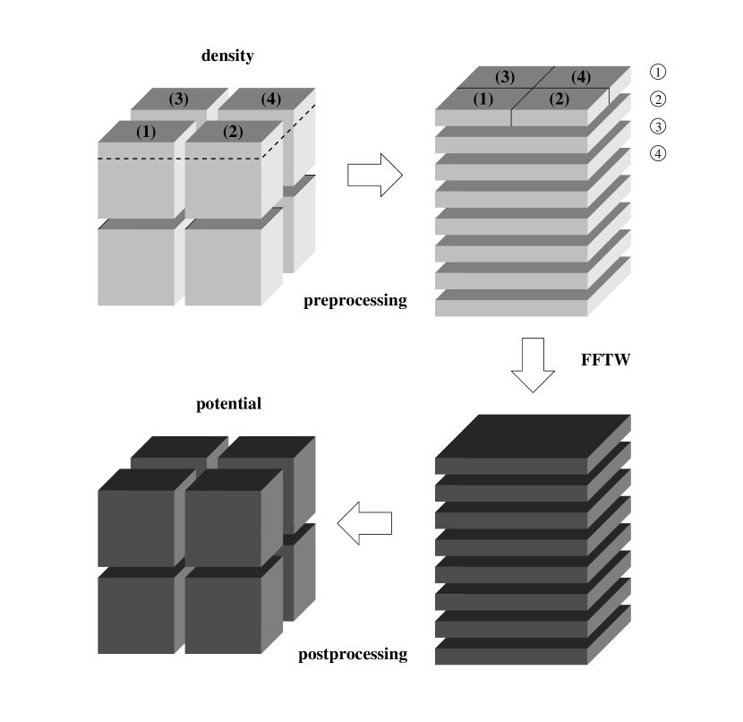
Figure 6.— Block-to-slab decomposition of density data before calling FFTW library and slab-to-block decomposition of gravitational potential afterward.

3.8.3 The Fast Fourier Transform Solver

As mentioned in §3.4, FFT algorithms offer a highly efficient method in solving the Poisson equation. The publicly available “Fastest Fourier Transform in the West” (FFTw) algorithm (Frigo & Johnson, 2005) is used as one of the gravity solvers available in ZEUS-MP. Note that the parallelized version of the FFTw library using MPI is only available in version 2.1.5 or before. Based on this version of MPI FFTw, the gravity solver implemented in ZEUS-MP  is valid only for Cartesian meshes with triply-periodic boundaries.

The transform data used by the FFTw routines is distributed, which means that a distinct portion of data resides in each processor during the transformation. In particular, the data array is divided along the first dimension of the data cube, which is sometimes called a slab decomposition. Users can design their data layout using slab decomposition as the FFTw requires but it is inconvenient for solving general problems. Therefore, there is a preprocessing of the density data distribution from a general block domain decomposition to a slab decomposition before calling the FFTw routines. After the potential is calculated, the slab decomposition of the potential is transformed back to block decomposition in the postprocessing stage. Figure 6 shows the idea of these two additional processes.

In figure 6, the initial density data block is first rearranged from block decomposition into slab decomposition. In this example using a 2 $\times$ 2 $\times$ 2 topology, the first layer of blocks will be divided into four slabs. The four processors exchange the data slabs to ensure the density data remains organized at the same spatial location. Therefore, the data exchange can be viewed as a rearrangement of the spatial location of processors. Since data in the second layer of blocks does not overlap with the first layer of data blocks, the non-blocking data communication among blocks in different layers can proceed simultaneously. After the gravitational potential is calculated, the reverse rearrangement of potential data from slab decomposition back to block decomposition is performed in an analogous manner.

Because of the required slab decomposition in FFTw, the number of processors that can be used for a given problem size is limited. For example, for a problem with 512³ zones on 512 processors, each slab least one cell thick. Using more than 512 processors in this example will not lessen the time to solution for the potential as extra processors would simply stand idle.

4. Verification Tests

In this section we present results from a suite of test problems designed to stress each of ZEUS-MP’s physics modules and verify the correct function of each. We begin with a pure HD problem which follows shock propagation in spherical geometry. We then examine a trio of MHD problems, two of which were considered in Stone & Norman (1992b), and the final of which has become a standard multidimensional test among developers of Godunov-based MHD codes. The section concludes with two radiation problems, the first treating radiation diffusion waves through static media; the second following the evolution of radiating shock waves. All problems with shocks use a quadratic (von Neumann-Richtmyer) artificial viscosity coefficient qcon of 2.0. The Orszag-Tang vortex test uses an additional linear viscosity with a value of qlin = 0.25.

Three of the test problems discussed below which include hydrodynamic effects are also adiabatic: these are the Sedov-Taylor HD blast wave, the MHD Riemann problem, and the Orszag-Tang MHD vortex problem. In these cases, the total fluid energy integrated over the grid should remain constant. Because ZEUS-MP  evolves an internal gas energy, rather than total fluid energy, equation, the ZEUS-MP solution scheme is non-conservative by construction. It therefore behooves us to monitor and disclose errors in total energy conservation as appropriate. For the three adiabatic dynamics problems noted above, the total energy conservation errors (measured relative to the initial integrated energy) were 1.4%, 0.8%, and 1.6%, respectively.

For problems involving magnetic field evolution, an additional metric of solution fidelity is the numerical adherence to the divergence-free constraint. As shown analytically in §3.2 and previously in Hawley & Stone (1995); Stone & Norman (1992b); Evans & Hawley (1988), the Constrained Transport algorithm is divergence-free by construction, regardless of the method chosen to compute the EMF’s. Nonetheless, all numerical codes which evolve discrete representations of the fluid equations are vulnerable to errors bounded from below by machine round-off; we therefore compute ${\bf\nabla\cdot}{\bf B}/|{\bf B}|$ at each mesh point and record the largest positive and negative values thus obtained. For the Alfvén rotor and MHD Riemann problems, which are computed on 1D grids, the maximum normalized divergence values at the end of the calculations remain formally zero to machine tolerance in double precision (15 significant figures). For the 2D Orszag-Tang vortex, the divergence-free constraint remains satisfied to within roughly 1 part in 10¹², consistent with machine round-off error over an evolution of roughly 1000 timesteps.

4.1. Hydrodynamics: Sedov-Taylor Blast Wave

Figure 7.— Density vs. radius for the Sedov-Taylor blast wave. Density is plotted in units of $10^{-8}$ g cm^-3; radius is plotted in units of $10^{13}$ cm. Profiles represent numerical results plotted in intervals of $6\times 10^{4}$ seconds. The dashed line shows the analytic value for the peak density.

Our first test problem is a classic hydrodynamic test due to Sedov (1959), in which a point explosion is induced at the center of a cold, homogeneous sphere in the absence of gravity. Problem parameters are chosen such that the explosion energy is orders of magnitude larger than the total internal energy of the cloud. In this case, the resulting shock wave evolves in a self-similar fashion in which the shock radius and velocity evolve with time according to

$$r_{sh}\ =\ \xi_{sh}\left(E_{o}\over\rho_{o}\right)^{1/5}t^{2/5},$$ (71)

and

$$v_{sh}\ =\ {2\over 5}\xi_{sh}\left(E_{o}\over\rho_{o}\right)^{1/5}t^{-3/5},$$ (72)

where $E_{o}$ and $\rho_{o}$ are the explosion energy and the initial density, respectively. $\xi_{sh}$ is a dimensionless constant which is equal to 1.15 for an ideal gas with $\gamma=5/3$. The density, pressure, temperature, and fluid velocity at the shock front are given by

$$\rho_{s}\ =\ 4\rho_{o},$$ (73)

$$P_{s}\ =\ {3\over 4}\rho_{o}v^{2}_{sh},$$ (74)

$$T_{s}\ =\ {3\over 16}{\mu m_{h}\over k_{B}}v^{2}_{sh},$$ (75)

and

$$v_{s}\ =\ {3\over 4}v_{sh}.$$ (76)

Figure 8.— Shock radius vs. time for the Sedov-Taylor blast wave. Time is plotted in units of 10⁴ seconds in the right-hand figure. Open circles represent numerical results plotted at the times corresponding to profiles in Figure 7. The solid line indicates the analytic solution.

Our problem was run in one dimension on a mesh of 500 zones equally spaced in radius. We initialize a spherical cloud of radius 10¹⁴ cm with a uniform density of 10^-8 g/cm³. The initial temperature is 50 K. At t = 0, 10⁵⁰ ergs of internal energy are deposited within a radius of 10¹² cm, which spreads the blast energy over 5 zones. Depositing the energy over a few zones within a small region centered on the origin maintains the point-like nature of the explosion and markedly improves the accuracy of the solution relative to that obtained if the all of the energy is deposited in the first zone.

Figures 7 and 8 provide results of our Sedov-Taylor blast wave test. Figure 7 shows radial plots of density separated in time by $6\times 10^{4}$ seconds. The density and radius are expressed in units of $10^{-8}$ g/cm^-3 and cm, respectively. The dashed line indicates the analytic value for the density at the shock front. Figure 8 shows numerical values (open circles) of the shock front at times identical to those used in the Figure 7. These data are superimposed upon the analytic solution (solid line) for the shock radius given by equation 71.

4.2. MHD

4.2.1 Magnetic Braking of an Aligned Rotor

Figure 9.— MHD aligned rotor: angular velocity vs. Z. The dashed line indicates the analytic solution of Mouschovias & Paleologou (1980).

Figure 10.— MHD aligned rotor: $B_{\phi}$ vs. Z. The dashed line indicates the analytic solution of Mouschovias & Paleologou (1980).

Figure 11.— MHD Riemann problem: density vs. X at t = 80 sec.

Figure 12.— MHD Riemann problem: 1-velocity vs. X at t = 80 sec.

Figure 13.— MHD Riemann problem: 2-velocity vs. X at t = 80 sec.

Our first MHD test examines the propagation of torsional Alfvén waves generated by an aligned rotor. A disk of uniform density $\rho_{d}$, thickness $z_{d}$, and angular velocity $\Omega_{0}$ lies in an ambient, initially static, medium with density $\rho_{m}$. The disk and medium are threaded by an initially uniform magnetic field oriented parallel to the rotation axis of the disk. Considered in cylindrical geometry, rotation of the disk produces transverse Alfvén waves which propagate along the Z axis and generate non-zero $\phi$ components of velocity and magnetic field. Analytic solutions for $v_{\phi}$ and $B_{\phi}$ were calculated by Mouschovias & Paleologou (1980) under the assumption that only the transverse Alfvén wave modes are present; to reproduce these conditions in ZEUS-MP, compressional wave modes due to gradients in gas and magnetic pressures are artificially suppressed. The utility of this restriction lies in the fact that in more general calculations, errors in the propagation of Alfvén waves may easily be masked by the effects of other wave modes in the problem.

The problem parameters as described above correspond to the case of discontinuous initial conditions considered in Mouschovias & Paleologou (1980). We consider a half-plane spanning the range $0~{}\leq~{}Z~{}\leq~{}15$, with $\rho_{d}$ = 10 and $\rho_{m}$ = 1. Because there are no dynamical phenomena acting along the radial coordinate, we may compute the problem on a 1-D grid of Z on which $R$- and $\phi$-invariant values of $v_{\phi}$ and $B_{\phi}$ are computed. Figures 9 and 10 show results of the calculation at a time t = 13. Solid curves indicate the solutions from ZEUS-MP; dashed lines show the analytic solution of Mouschovias & Paleologou (1980). These results are consistent with those obtained with ZEUS-2D and shown in Stone & Norman (1992b); the only salient difference between the two calculations is that we used twice as many zones (600) as reported for the ZEUS-2D calculation. The increased resolution is mandated by the fact that the HSMOCCT algorithm is by construction more diffusive than the original MOCCT algorithm documented in Stone & Norman (1992b). As noted previously in section 3.2 and discussed in detail in Hawley & Stone (1995), this added diffusivity makes the MOCCT algorithm more robust in fully multidimensional calculations. The requirement within HSMOCCT of higher resolution with respect to ZEUS-2D’s older MOCCT algorithm is maximized in this test problem due to the artificial suppression of compressive hydrodynamic waves and longitudinal MHD waves; the true resolution requirements of HSMOCCT as implemented in ZEUS-MP will depend in part upon the relative importance of various wave modes to the calculation and will in general be problem dependent.

4.2.2 MHD Riemann Problem

Figure 14.— MHD Riemann problem: 3-velocity vs. X at t = 80 sec.

Figure 15.— MHD Riemann problem: 2-component of magnetic field vs. X at t = 80 sec.

Figure 16.— MHD Riemann problem: 3-component of magnetic field vs. X at t = 80 sec.

Our second MHD problem is a magnetic shock tube problem due to Brio & Wu (1988). Test results with ZEUS-2D using the van Leer advection algorithm were also published in Stone & Norman (1992b). This test problem is described by “left” and “right” states in which the discontinuous medium is threaded by a magnetic field which is uniform on both sides but exhibits a kink at the material interface. Our formulation of the problem differs from that of Brio & Wu (1988) and Stone & Norman (1992b) only in that we have oriented the transverse component of the magnetic field to have non-zero components along both the Y and Z axes in Cartesian geometry. At t = 0, our left state is given by $\left(\rho_{l},~{}p_{l},~{}B_{l}^{x},~{}B_{l}^{y},~{}B_{l}^{z}\right)$ = (1.0, 1.0, 0.75, 0.6, 0.8), and the right state is given by $\left(\rho_{r},~{}p_{r},~{}B_{r}^{x},~{}B_{r}^{y},~{}B_{r}^{z}\right)$ = (0.125, 0.1, 0.75, -0.6, -0.8). All velocities are initially zero. The ratio of specific heats for this problem is 2.0. As with the calculation in Stone & Norman (1992b), the problem is computed in 1-D on an 800-zone grid and run to a time of t = 80. The spatial domain length is 800.

Figures 11 through 16 show the results obtained with ZEUS-MP. The 1-component of $B$ (not included in the figures) remained flat over the domain at its initial value, as expected. The grid resolution is identical to that used in the ZEUS-2D calculation, and the results are evidently consistent (see Fig. 6 of Stone & Norman (1992b)). While this problem is not truly multidimensional, it does exhibit both transverse and compressional wave modes, in contrast with the previous test problem. In this case, we may qualitatively match the results from ZEUS-2D without an increase in grid resolution.

4.2.3 Orszag-Tang Vortex

Our final MHD test problem is a multidimensional problem due to Orszag & Tang (1979) which has been featured in a number of recent MHD method papers, such as  Dai & Woodward (1998); Ryu et al. (1998) and Londrillo & Del Zanna (2000); Londrillo & del Zanna (2004). This problem follows the evolution of a 2-D periodic box of gas with $\gamma$ = 5/3, in which fluid velocities and magnetic field components are initialized according to ${\bf v}~{}=~{}v_{0}\left[-\sin\left(2\pi y\right)\hat{\bf x}+\sin\left(2\pi x\right)\hat{\bf y}\right]$ and ${\bf B}~{}=~{}B_{0}\left[-\sin\left(2\pi y\right)\hat{\bf x}+\sin\left(4\pi x\right)\hat{\bf y}\right]$, with $v_{0}$ = 1 and $B_{0}$ = 1/$(4\pi)^{1/2}$. The box has length 1.0 along each side. The density and pressure are initially uniform with values of 25/(36$\pi$) and 5/(12$\pi$), respectively (these choices lead to an initial adiabatic sound speed of 1.0). Subsequent evolution leads to a complex network of waves, shocks, rarefactions, and stagnant flows. Ryu et al. (1998) provide greyscale snapshots of the flow field at t = 0.48; in addition, they provide 1-D cuts through the data along the line given by $y$ = 0.4277, over which the gas and magnetic pressures are plotted as functions of $x$. The Ryu et al. (1998) results were computed on a 256²-zone Cartesian mesh. For consistency, we also computed the problem on a 256²-zone mesh, from which comparison values of pressure at the identical cut in $y$ may be extracted. To explore the effect of resolution, we also provide 2-D greyscale images from a 512²-zone calculation.

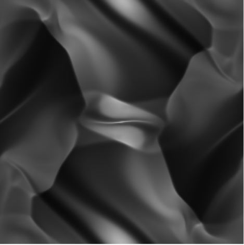
Figure 17.— Orszag-Tang vortex: pressure at t = 0.48 seconds. 256² zones were used.

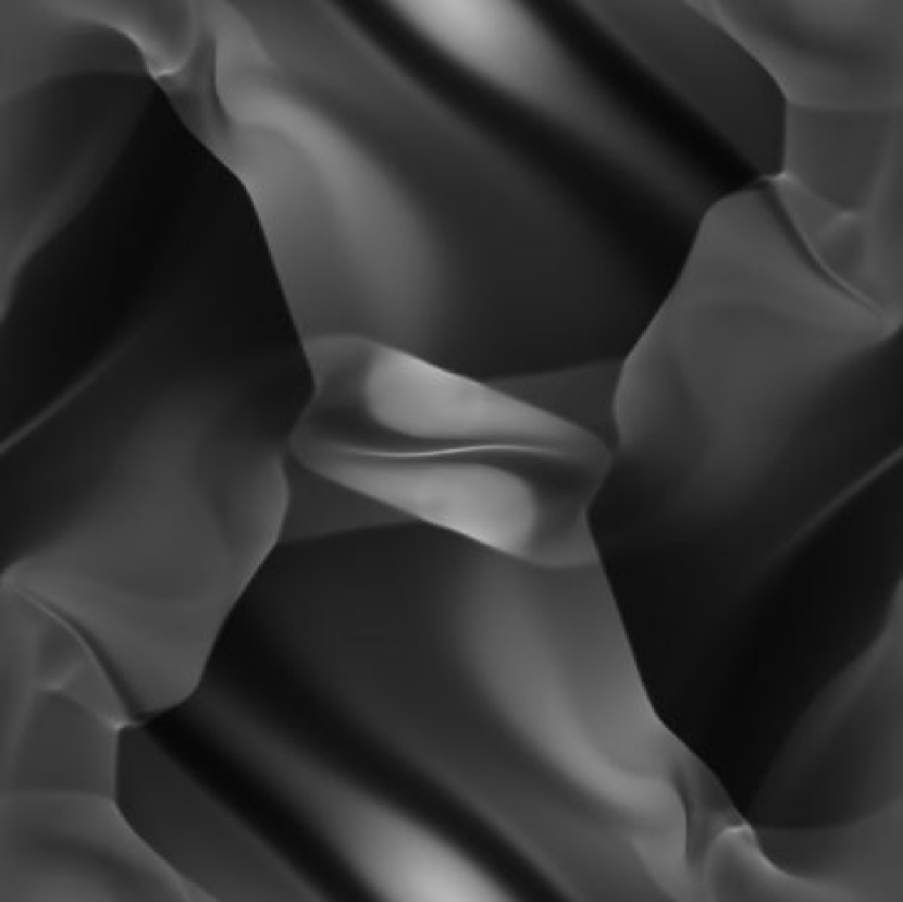
Figure 18.— Orszag-Tang vortex: pressure at t = 0.48 seconds. 512² zones were used.

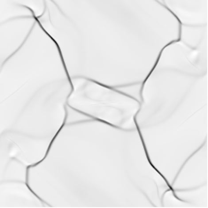
Figure 19.— Orszag-Tang vortex: $\nabla\cdot{\bf v}$ at t = 0.48 seconds for the 256² zone calculation.

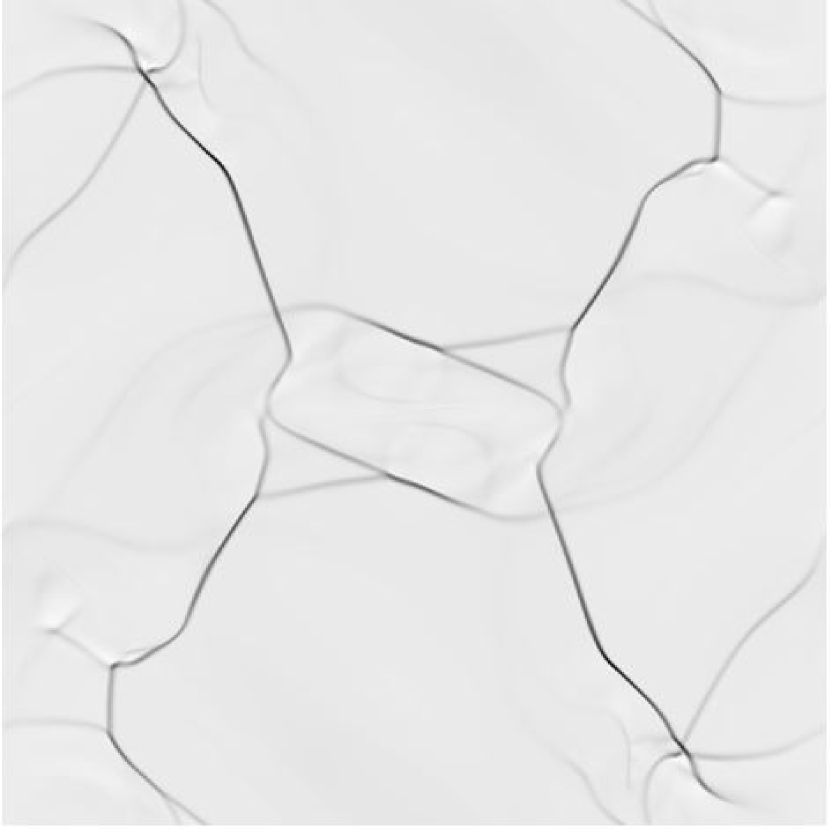
Figure 20.— Orszag-Tang vortex: $\nabla\cdot{\bf v}$ at t = 0.48 seconds for the 512² zone calculation.

Our multidimensional flow structures at t = 0.48 are given in Figures 17 through 20, which are to be compared to the grey-scale panels on the left-hand side of Figure 3 in Ryu et al. (1998). Figure 21 presents line plots of gas and magnetic pressure along a line of $x$ located at $y$ = 0.4277. Save for a very small notch in the gas pressure near x = 0.5, our pressure profiles from the 256² calculation appear to be virtually identical to those from  Ryu et al. (1998) at identical resolution. With respect to the 2-D images, the effect of resolution is most apparent in maps of the velocity divergence (Figures  19 and 20). Again, the ZEUS-MP results at a grid resolution of 256² compare quite favorably to those from Ryu et al. (1998), with subtle flow features marginally less well resolved. Our results are likewise consistent with those computed at similar resolution by Dai & Woodward (1998) and Londrillo & Del Zanna (2000) (Londrillo & del Zanna (2004) also computed the problem but did not include figures matching the other cited works). The 256² and 512² results clearly bracket those of Ryu et al. (1998); thus we see that in this problem axial resolution requirements of the two codes differ by at most a factor of 2, which we consider an agreeable result for a finite-difference staggered-mesh code.

Figure 21.— Gas and magnetic pressures vs. $x$ along $y$ = 0.4277 at time t = 0.48 sec.

4.3. Radiation

4.3.1 Marshak Waves

We begin our examination of radiation physics with a test problem emphasizing the coupling between matter and radiation. The Marshak wave problem we compute was formulated by Su & Olson (1996) after a description in Pomraning (1979). The problem considers the heating of a uniform, semi-infinite slab initially at $T=0$ everywhere. The material is characterized by a $T$-independent (and therefore constant) opacity ($\kappa$) and a specific heat ($\alpha$) proportional to $T^{3}$, in which case the gas and radiation energy equations become linear in the quantities ${\rm E}$ and $T^{4}$. Pomraning defined dimensionless space and time coordinates as

$$x\ \equiv\ \sqrt{3}\kappa z,$$ (77)

and

$$\tau\ \equiv\ \left({4ac\kappa\over\alpha}\right)t,$$ (78)

and introduced dimensionless dependent variables, defined as

$$u(x,\tau)\ \equiv\ \left(c\over 4\right)\left[E(z,t)\over F_{\rm inc}\right],$$ (79)

and

$$v(x,\tau)\ \equiv\ \left(c\over 4\right)\left[aT^{4}(z,t)\over F_{\rm inc}\right].$$ (80)

In (79) and (80), $F_{\rm inc}$ is the incident boundary flux. With the definitions given by (77) through (80), Pomraning showed that the radiation and gas energy equations could be rewritten, respectively, as

$$\epsilon{\partial u(x,\tau)\over\partial\tau}-{\partial^{2}u(x,\tau)\over\partial x^{2}}\ =\ v(x,\tau)-u(x,\tau),$$ (81)

and

$${\partial v(x,\tau)\over\partial\tau}\ =\ u(x,\tau)-v(x,\tau),$$ (82)

subject to the following boundary conditions:

$$u(0,\tau)-{2\over\sqrt{3}}{\partial u(0,\tau)\over\partial x}\ =\ 1,$$ (83)

and

$$u(\infty,\tau)\ =\ u(x,0)\ =\ v(x,0)\ =\ 0.$$ (84)

The user-specified parameter $\epsilon$ is related to the radiation constant and specific heat through

$$\epsilon\ =\ {4a\over\alpha}.$$ (85)

Figure 22.— Curves of log(U) and log(V) vs. log(X) for 2 values of $\tau$. Curves show analytic solutions; circles indicate numerical data.

With a choice of $\epsilon$, the problem is completely specified and may be solved both numerically and analytically. For the ZEUS-MP test, we chose a 1-D Cartesian grid with 200 zones and a uniform density of 1 g cm^-3. The domain length is set to 8 cm, and the photon mean-free path ($\kappa^{-1}$) is chosen to be 1.73025 cm. Because this problem was designed for a pure diffusion equation, no flux limiters were used in the FLD module. $\epsilon$ was chosen to be 0.1, allowing direct comparison between our results and those given by Su & Olson (1996). Our results are shown in Figure 22, in which the dimensionless energy variables $u$ and $v$ are plotted against the dimensionless space coordinate $x$ at two different values of the dimensionless time, $\tau$. The open circles indicate benchmark data taken from the tabulated solutions of Su & Olson (1996); solid curves indicate ZEUS-MP results. The agreement is excellent.

4.3.2 Radiating Shock Waves

Figure 23.— Subcritical radiating shock; matter and radiation temperatures vs. comoving X coordinate. Plot times are 5400, 1.7$\times 10^{4}$, 2.8$\times 10^{4}$, and 3.8$\times 10^{4}$ seconds.

The classic text on the theory of shock waves and associated radiative phenomena is due to Zel’Dovich & Raizer (1967) (see also Zel’Dovich & Raizer (1969) for a short review article on shock waves and radiation). A more recent summary of basic concepts is available in Mihalas & Mihalas (1984). Radiating shock waves differ qualitatively from their purely hydrodynamic counterparts due the presence of a radiative precursor created by radiative preheating of material upstream from the shock front. The existence of this precursor gives rise to the identification of so-called subcritical and supercritical radiating shocks, which are distinguished by a comparison of the gas temperature behind the shock front to that in the material immediately upstream from the shock. In the case of subcritical shocks, the post-shock gas temperature exceeds the upstream value, and the radiative precursor is relatively weak. As the shock velocity is increased beyond a critical value, however, the upstream gas temperature becomes equal to (but never exceeds) the post-shock temperature; such shocks show very strong radiative preheating of the unshocked gas and are identified as supercritical shocks.

Figure 24.— Supercritical radiating shock; matter and radiation temperatures vs. comoving X coordinate. Plot times are 860, 4000, 7500, and 1.3$\times 10^{4}$ seconds.

A numerical prescription for radiating shock test problems appropriate for astrophysical simulation codes was published by Ensman (1994); this configuration was revisited by Gehmeyr & Mihalas (1994) and again by Sincell et al. (1999a, b) and Hayes & Norman (2003). In this model, a domain of length or radius $7\times 10^{10}$ cm and an initially uniform density of $7.78\times 10^{-8}$ g cm^-3 is given an initial temperature profile such that $T$ falls smoothly from a value of 85 K at the inner boundary to 10 K at the outer boundary. The non-zero gradient was necessary to avoid numerical difficulties in Ensman’s VISPHOT code. A constant opacity of $3.1\times 10^{-10}$ is chosen, which yields a photon mean-free path roughly 5% of the domain length. Because the VISPHOT code uses a Lagrangean mesh, the shock is created by a “piston” affected by choosing an inner boundary condition on the fluid velocity. ZEUS-MP recreates this condition on an Eulerian grid by initializing the fluid velocity throughout the domain and outer boundary to the (negative of) the required piston velocity. The subcritical shock and supercritical shock tests share all problem parameters save for the piston velocity, chosen to be 6 km/s in the former case and 20 km/s for the latter. 512 zones were used to execute the problem on a 1-D mesh.

Figures 23 and 24 present temperature profiles for the subcritical and supercritical cases, respectively. To aid comparison of our Eulerian results to the Lagrangean results of Ensman (1994), we transform the coordinate axis into the rest frame of the unshocked matter. Solid lines indicate gas temperature; dashed lines indicate a radiation “temperature” defined by $T_{r}\equiv\left({\rm E}/a_{r}\right)^{1/4}$, where $a_{r}$ is the radiation constant. Note the strongly preheated material ahead of the shock front in the supercritical case. Our results were computed in Cartesian geometry; those from Ensman (1994) were computed in a thin spherical shell with a large radius of curvature. This problem was also treated by Hayes & Norman (2003) using ZEUS-MP coupled to a parallel VTEF algorithm. Because that code was designed specifically for 2-D cylindrically-symmetric problems, the problem geometry was different in that the radiating surface was planar yet of finite transverse extent, whereas these results consider a formally infinite plane. This difference results in somewhat different peak values for temperature, but otherwise the results are qualitatively consistent.

5. Performance Tests

Section 4 considered test problems which gauge the accuracy of the code. This section considers issues of numerical performance, with a particular emphasis on problems distributed among large numbers of parallel processors.

5.1. Aspects of Scalability

The topic of parallel performance is most often encapsulated in the notion of scalability, which in this context is typically assessed by measuring the reduction in CPU time for a given quantity of numerical work as this work is distributed among an increasing number of processors. Relative to the cost on one CPU, perfect scalability would be represented by a cost reduction factor of $1/N$ when the same job is distributed across N processors. For tasks in which each processor can operate upon its portion of data independently of all other processors (a so-called embarrassingly parallel operation), perfect scalability is trivially achieved. Algorithms which compute solutions to spatially-discretized PDE’s are by construction not embarrassingly parallel because the discrete spatial derivative operators employ stencils that overlap processor tile boundaries along the tile edges. On distributed-memory computers, data communication will therefore be required. Efficient management of this communication is thus a key ingredient to an efficient parallelization strategy.

More generally, scalability describes the sensitivity of an algorithm’s CPU cost to a number of factors, of which parallelism is a leading but by no means unique member. Section 3.8.2 compared the cost of MG linear solvers to traditional stationary methods for a given problem size; the costs of the two methods exhibit very different dependencies upon the number of unknowns in the linear system. For iterative methods such as CG and MG, the required number of iterations for a converged solution is the primary factor in algorithm cost. Solvers whose iteration counts vary more weakly with problem size are to be favored for very large problems. In ideal cases, the required number of iterations for convergence of an MG solver can be virtually independent of the problem size, thus MG is often said to scale well to large problems. Because this behavior is orthogonal to the issue of parallel decomposition, we identify this as an independent definition of scalability.

Table 2Radiation Diffusion Test Parameters.

Medium	Outer Radius (cm)	$\rho$ (g/cm3)	Temperature (eV)
D-T gas	0.087	0.025	000.025
D-T ice	0.095	0.250	000.025
C-H foam	0.111	1.200	000.025
He gas	0.490	0.010	300.000

An additional factor bearing on the cost of an iterative linear system solution is diagonal dominance, a condition in which matrix elements along the main diagonal are much larger in magnitude than off-diagonal elements along a given row. Matrices resulting from the discretization of the time-dependent diffusion equation exhibit diagonal dominance that varies directly with the size of the time step. To see this, consider the static diffusion equation discretized on a 1-D mesh with uniform spacing, $\Delta x$. For a static medium, the radiation energy equation becomes

$${\partial{\rm E}\over\partial t}-\nabla\cdot D\nabla{\rm E}\ =\ S,$$ (86)

where $S$ contains local source terms. We assume a spatially uniform medium (yielding a spatially constant D) and write this equation in discrete form as

$${{{\rm E}^{n+1}_{i}-{\rm E}^{n}_{i}}\over{\Delta t}}-\left[D\over(\Delta x)^{2}\right]\left({\rm E}^{n+1}_{i+1}-2{\rm E}^{n+1}_{i}+{\rm E}^{n+1}_{i-1}\right)\ =\ S_{i},$$ (87)

which may be rearranged to make the linear system structure obvious:

$$- \left[D{\Delta t}\over(\Delta x)^{2}\right]{\rm E}^{n+1}_{i-1}+\left[1+{2D{\Delta t}\over(\Delta x)^{2}}\right]{\rm E}^{n+1}_{i}$$ (88)

$$- \left[D{\Delta t}\over(\Delta x)^{2}\right]{\rm E}^{n+1}_{i+1}\ =\ {\rm E}^{n}_{i}+S_{i}{\Delta t}.$$

The relationship between time step and diagonal dominance is manifest: in the limit that ${\Delta t}\rightarrow 0$, the linear system represented by (88) reduces to the identity matrix! In the opposite limit, the off-diagonal elements are comparable in magnitude to the main diagonal, a situation which results in greatly increased numbers of iterations required for convergence in a CG linear solver such as that implemented in our FLD module.

Figure 25.— Radiation diffusion (1D): profiles of radiation temperature (solid lines) and gas temperature (dashed lines) at times of 0.0, 0.1, 0.5, 0.7, 1.0, and 10 ns. The initial profiles are step functions with the discontinuities located at R = 0.11 cm. The radiation wave propagates leftward, with the gas temperature lagging the radiation temperature, particularly in the optically thick regions.

Figure 26.— Radiation diffusion (1D): logarithms of the time step (solid line) and mean number of CG iterations per N-R iteration (dashed line) as functions of the evolution time. Times are measured in seconds.

We demonstrate this behavior with a radiation diffusion problem in which a cold sphere is immersed in a high-temperature radiation field. Problem parameters are given in Table 2. The initial values of density and temperature are taken from a test problem given in Hayes & Norman (1999) designed to qualitatively mimic features of an Inertial Confinement Fusion (ICF) simulation such as that used by Baldwin et al. (1999) to compare numerical performance of CG-based and MG-based linear system solvers. The irradiated sphere is constructed of layers with strongly disparate densities and photon mean-free paths. The actual physical system this problem imitates (albeit crudely) is a sphere of D-T gas surrounded by a solid D-T “ice” of higher density, itself surrounded by a carbon-hydrogen foam of yet higher density. This assembly is immersed in a low density He gas subjected at t = 0 to an intense radiation field with a characteristic temperature of 300 eV. Opacities for real ICF materials have complex dependencies on energy and composition; our toy problem captures the gross features of the mean-free path variation via the following expression:

$$\Lambda(\rho,T)\ =\ \Lambda_{0}\left(\rho\over\rho_{0}\right)^{\nu}\left(T\over T_{0}\right)^{\mu},$$ (89)

with $\Lambda_{0}$, $\rho_{0}$, $T_{0}$, $\nu$, and $\mu$ given by 10^-6, 1.2 g/cm³, 0.025 eV, 2.0, and 1.2, respectively. A further restriction is placed on the resulting opacities such that the minimum and maximum allowed values of $\chi$ are 10 and 10⁶ cm^-1. This restriction filters out unphysically high and low values of the absorption coefficients. The important feature of this problem is that low-density gas is surrounded by two solids of much higher (and differing) densities. This construction results in an inward-propagating radiation diffusion wave with a highly variable rate of progress. Snapshots of the gas and radiation temperatures at times of 0, 0.1, 0.5, 0.7, 1.0, and 10 nanoseconds are given in Figure 25. Histories of the time step and average number of CG iterations required for NR iteration in the FLD module are plotted against evolution time in Figure 26. The choppy appearance of the plots is an artifact of sampling (every tenth cycle was archived for plotting). For static diffusion problems or RHD problems characterized by rapidly time-varying radiation fields, evolution of the time step will be strongly constrained by the maximum allowed fractional change in the radiation energy (= 0.01 in this problem). The initial time step progression is upward as the exterior radiation field slowly diffuses through the opaque foam layer. By 0.5 ns, the radiation has diffused through the foam layer and begun to penetrate the less opaque D-T ice layer, at which time the time step drops sharply owing to the more rapid evolution of the radiation energy. The time step trends upward again until the radiation wave breaks through the D-T gas/ice boundary. The time step then drops again as the radiation streams into the central region. The final evolution of the time step is upward as the problem domain reaches its final equilibrium. The equilibrium temperature is lower than the initial exterior value because a reflecting outer boundary was chosen rather than an imposed boundary flux.

The dashed line in Figure 26 shows that the number of CG linear system iterations required to solve the FLD matrix during an outer N-R iteration closely parrots the time step behavior. This is understood as a natural consequence of time-dependent diagonal dominance of the matrix as illustrated by equation 88. This exercise demonstrates the existence of a third dimension of scalability of particular relevance to time-dependent simulations: the dependence of CPU cost upon time step size. When a linear system is very nearly diagonal, both CG and MG will converge rapidly, but because a single iteration of full MG is more expensive than a single CG iteration, one may expect situations in which CG presents a more economical solution strategy for a given problem size. That increasing time step size could provide a “cross over” point with regard to optimal method is a logical consequence. This issue was investigated extensively by Baldwin et al. (1999) in the context of 2-D RHD simulations in spherical geometry. They considered RHD problems in which the time step varied naturally by orders of magnitude during the course of the simulation, and noted indeed that no one method provided the best economy over the entire calculation. While adaptive selection of linear solvers in a particular physics module has not been implemented in ZEUS-MP, we note that experimention along such lines in the context of astrophysical problems is an enticing candidate for future research.

5.2. Parallel Performance Results

Figure 27.— Strong-scaling comparison: relative speedup vs. number of CPUs for problems of fixed size. The solid curves indicates perfect N-fold scaling with CPU count. 256³ zones were used for each problem; the maximum CPU number was 1024 for each case.

We explore additional aspects of algorithm performance with a quartet of test problems computed on 3-D grids with 256³ zones. The first two problems used are non-magnetic and magnetic variants of a simple blast wave test in which a sphere with initial overdensity and overpressure ratios of 100 and 10⁶ is defined with respect to a uniform background medium. The problem is defined on a Cartesian grid. The magnetic version augments the problem setup with a uniform magnetic field aligned with the Z axis. The third problem is a 3-D calculation of radiation diffusion into an ICF capsule, with problem parameters as given previously. The fourth problem is the gravitational collapse of a pressureless cloud, using problem parameters given in Stone & Norman (1992a).

Table 3Fixed-Work Scaling: 256³ MHD (30 Time Steps)

Processors	CPU Time (sec)	Speedup	Parallel Efficiency (%)
0001	9391.00	—	—
0002	4624.00	0002.031	102
0004	2236.00	0004.200	105
0008	1097.00	0008.561	107
0016	0504.90	0018.600	116
0032	0248.10	0037.850	118
0064	0128.40	0073.140	114
0128	0064.60	0145.400	114
0256	0040.45	0232.200	090
0512	0021.84	0430.000	084
1024	0008.91	1053.000	103

Table 4Fixed-Work Scaling: 256³ HD (50 Time Steps)

Processors	CPU Time (sec)	Speedup	Parallel Efficiency (%)
0001	5256.000	—	—
0002	2746.000	0001.91	96
0004	1323.000	0003.97	99
0008	669.800	0007.85	98
0016	335.400	0015.70	98
0032	165.400	0031.80	99
0064	89.250	0058.90	92
0128	43.140	0122.00	95
0256	20.850	0252.00	98
0512	11.690	0450.00	88
1024	6.450	0815.00	80

For each problem, parallel performance is measured by a so-called strong-scaling test in which the total number of zones (and therefore the total amount of computational work) is held constant as the problem is repeated with increasing numbers of CPU’s. Each problem is run for a small number of cycles (typically 30 to 50) which is held fixed for each trial. Figure 27 and Tables 3, 4, 5, and 6 summarize the results for the MHD blast wave, HD blast wave, radiation diffusion, and gravitational collapse tests. The number of timesteps for which each test was run is indicated in the title of each table, from which single time step costs may be derived. In this example, the gravitational collapse problem solved Poisson’s equation with the CG linear solver, which is also used in the diffusion test. It is important to note that in this type of scaling study where the total problem size is held fixed, parallel scalability will inevitably break down for a sufficiently large number of processors, due in large part to surface-to-volume effects: when the local processor data block is too small, the communication cost of shipping data along the block’s surfaces will compete with the computational cost of processing the full block volume. The number processors necessary to induce a turnover in a code’s parallel scalability behavior will depend strongly on the level of communication required by the algorithm, a point we demonstrate in the experiments that follow. A competing technique for measuring scalability, known as a weak-scaling test, holds the processor block size constant and thus scales the total problem size with the number of processors. This alternative has some utility: if, for example, one determines that twice the grid resolution is required to satisfy a given accuracy metric, one may investigate if doubling the number of processors along the axis preserves the cost of computing a time step without degrading parallel performance. While this is a relevant consideration, we eschew weak-scaling studies in this paper because (1) with a sufficiently large block of data on each processor, even poor message-passing implementations of parallelism can perform reasonably well, and (2) the characteristics of the problem under study change as the zone number increases. For Courant-limited calculations, doubling the resolution will double the number of time steps needed to complete a calculation, which rather offsets the virtues of maintaining a constant cost per time step. For problems using implicit linear solvers, increasing the total number of zones will, to a degree depending on the solver method, increase the number of iterations required for convergence at each cycle. Strong-scaling studies, while providing a harsher test of a parallel implementation, speak directly to the question: how rapidly may a research problem of a given size be solved?

Table 5Fixed-Work Scaling: 256³ FLD (20 Time Steps)

Processors	CPU Time (sec)	Speedup	Parallel Efficiency (%)
0002	3184.000	—	—
0004	1569.000	002.03	102
0008	0887.100	003.59	090
0016	0509.800	006.25	078
0032	0269.900	011.80	074
0064	0146.900	021.70	068
0128	0071.120	044.80	070
0256	0036.380	087.50	068
0512	0020.150	158.00	062
1024	0012.380	257.00	050

Table 6Fixed-Work Scaling: 256³ Grav-CG (5 Time Steps)

Processors	CPU Time (sec)	Speedup	Parallel Efficiency (%)
0001	11430.00	—	—
0002	07013.00	001.63	82
0004	03696.00	003.09	77
0008	02300.00	004.97	62
0016	01666.00	006.86	83
0032	00866.50	013.20	41
0064	00422.80	027.00	42
0128	00184.80	061.90	48
0256	00076.97	149.00	58
0512	00067.47	169.00	33
1024	00047.64	240.00	23

The behaviors in Figure 27 reflect the relative impact of MPI communication operations on each module. The superlative scaling of the MHD tests derives from the highly computation-intensive nature of the algorithm. The HD test is actually a subset of the MHD problem, as both the MHD-specific routines and the HD advection algorithms must be used in any MHD problem. The radiation and gravity problems are both dominated by the cost of CG linear solver. The diffusion problem was run for a sufficiently limited number of time steps such that an average of eight CG iterations were required at each time step. In contrast, when used for the Poisson equation, of order 10² iterations are required for a mesh size of 256³. Because each CG iteration requires both MPI data exchanges at tile boundaries and global searches for error minima, high iteration counts result in very communication-intensive operations. Parallel efficiency, which is computed by dividing the speedup relative to 1 processor by the processor number, is displayed in the fourth column of Tables 3-6. Superlinear speedup is observed most dramatically for the MHD test; this behavior is a by-product of strong-scaling studies and arises because single-CPU performance is degraded when the local data chunk is too large to fit in a processor’s cache memory. This effect decreases as the per-CPU data size shrinks; the deleterious effects of communication then begin to appear as the processor counts run into the hundreds. Some of the peculiar variations in parallel efficiency in the MHD example are likely consequences of system and network effects associated with the particular machine used. Memory, bandwidth, and latency characteristic vary tremendously among different architectures; but the major trends shown in Figure 27 and the associated tables are representative and instructive, and are internally consistent with the relative reliance of each module upon data exchange among processors.

Figure 28.— A comparison of timings for the gravitational collapse problem in 3-D using the general CG solver and MGMPI’s multigrid solver for the Poisson equation.

The fact that the CG solver requires – irrespective of parallelism – more iterations for larger problems brings with it two liabilities: increased iteration counts boost both the total operation cost and the number of MPI messages sent and received. The fact that multi-grid methods exhibit convergence behavior with little sensitivity to problem size motivated us to implement the independently-developed MGMPI package for use as an alternative Poisson solver in ZEUS-MP. In its current form, MGMPI is restricted to 3-D Cartesian grids (which are nevertheless a common choice in large astrophysical calculations) with Dirichlet or Neumann boundary conditions (recall that the FFTw solver is offered for triply-periodic Cartesian meshes). Figure 28 shows the behavior of solution time against problem size for the gravitational collapse problem computed on a 3-D Cartesian mesh. Grid sizes of 63³, 127³, 255³, and 511³ zones were run. (Odd numbers of zones are required by the multigrid V-cycle in MGMPI.) Each trial was distributed across 64 processors to ensure that the larger problems would not exceed single-CPU memory limits. At small grid sizes, the CG solver is less expensive than the MGMPI solution, but at a mesh size of 511³ the CG solution has clearly diverged with respect to the MGMPI solver. The fundamental difference lies in the average number of solver iterations required per time step. For the CG solver, this number was 32, 56, 99, and 190, respectively, for the four problem sizes tested. For MGMPI, this number is 2.2 for the smallest problem and grows only to 3 for the 511³ run. Despite MGMPI’s fairly high operation cost per iteration, the insensitivity of its convergence behavior to problem size guarantees, for a given parallel distribution, a performance advantage over the CG solver for a sufficiently large problem. In its current form, MGMPI does not employ asynchronous MPI calls for its message passing, as does the CG solver. The problem size for which MGMPI enjoys a clear advantage over the CG solver may therefore depend in part on the number of processors chosen. Nonetheless, for very large problems involving self-gravity on a Cartesian mesh, MGMPI is likely to be the preferred option in a ZEUS-MP calculation.

6. Summary

In the introduction, we advertised the theme of this paper as “physics, flexibility, and parallelism.” That these features are defining traits of ZEUS-MP is manifest: hydrodynamics, MHD, and radiation diffusion may be deployed, singly or in concert, on Cartesian, cylindrical, or spherical meshes in one to three dimensions. ZEUS-MP demonstrates parallel scalability suitable for computing platforms ranging from small clusters to the largest platforms currently available for unclassified research. Features of a code designed for community use must also include accuracy and computational expediency. The accuracy of ZEUS-MP has been verified both by traditional test problems and a multidimensional MHD problem frequently touted by developers of Godunov-based MHD codes. Even when additional resolution is required to ensure accuracy of a calculation, ZEUS-MP’s parallel performance provides a powerful mechanism for keeping the required solution times manageable.

Virtues notwithstanding, we note that there are several ways in which ZEUS-MP may be modified and improved within its solution paradigm. Non-ideal MHD effects such as Ohmic dissipation and ambipolar diffusion are requisite in a variety of topics in interstellar physics such as star formation and interstellar shocks; methodologies for including these effects in the ZEUS framework have been documented by Stone (1999) in the case of Ohmic dissipation and likewise by Stone (1997) for ambipolar diffusion. A 3-D version of the VTEF algorithm described by Hayes & Norman (2003) would be a major undertaking, but we note an approximation suggested by Ruszkowski & Begelman (2003) as an improvement to FLD suitable for the ZEUS codes. Because ZEUS-MP is intended for public distribution, one mission of this paper is to provide reference documentation at a sufficiently high level of detail so that ambitious code developers may modify it for their particular needs.

An additional area of improvement in which we are currently engaged concerns the iterative solvers offered with the code. The much higher computational cost of simulations with FLD and the CG-based self-gravity module derives from the very high numbers of iterations required for the CG linear solver to converge when the matrix loses its diagonal dominance. Because the matrix generated by the discrete Poisson equation is never strongly diagonally dominant, CG methods lose favor as the tool of choice for the Poisson problem on large grids. The suitability of CG to radiation problems is very dependent on the physical and temporal character of the problem at hand. As shown by Baldwin et al. (1999), suitably optimized MG methods may be preferable to CG for some classes of radiation problems. Our current MGMPI solver is not yet flexible enough for use in radiation applications, but enlarging its scope of applicability is a high priority item for future research.

We also note that the convergence requirements of our current CG solver may be dramatically improved with the use of a more effective preconditioner (recall the discussion in §3.8.1). Our solver uses diagonal preconditioning, which simultaneously boasts maximal ease of implementation and minimal range of effectiveness with respect to the condition numbers for which convergence is notably improved. Despite the importance of preconditioning to the performance of linear solvers upon which many astrophysical simulations must depend, this topic has received relatively little attention in the numerical astrophysics literature. One study which has focused on astrophysical applications was performed by Swesty et al. (2004), who considered a class of preconditioners known as “sparse approximate inverse” (SPAI) preconditioners. As the name implies, SPAI preconditioners attempt to construct an approximation to the inverse of a matrix which is more sophisticated than the purely diagonal approximation, but far less expensive to compute than the full inverse. Swesty et al. (2004) have constructed SPAI preconditioners designed for the linearized, discrete, energy-dependent version of the FLD equation, the so-called multigroup flux-limited diffusion (MGFLD) equation. The scientific focus in the Swesty et al. (2004) paper is on 2-D and 3-D MGFLD linear systems written to compute multidimensional neutrino diffusion coupled to hydrodynamic flows in core-collapse supernova simulations. While their analysis is designed for the MGFLD equations, they consider special cases of isoenergetic diffusion directly analogous to the reduced system of energy-averaged (or “grey”) FLD equations adopted in ZEUS-MP (and ZEUS-2D). The results reported in Swesty et al. (2004) suggest that SPAI preconditioners may offer a very profitable line of research for future FLD implementations in ZEUS-MP or other application codes.

Appendix A A Map of ZEUS-MP

Table 7The Mapping Between ZEUS-MP Subroutines and Equations Solved.

Action	Equation	Routine	Hydro	MHD	RHD
Compute $\Phi$	E21	GRAVITY	$\surd$	$\surd$	$\surd$
SRCSTEP Updates
$v1_{i,j,k}$ force update	B10	FORCES	$\surd$	$\surd$	$\surd$
$v2_{i,j,k}$ force update	B11	FORCES	$\surd$	$\surd$	$\surd$
$v3_{i,j,k}$ force update	B12	FORCES	$\surd$	$\surd$	$\surd$
$v1_{i,j,k}$ viscosity update	B41	AVISC	$\surd$	$\surd$	$\surd$
$v2_{i,j,k}$ viscosity update	B42	AVISC	$\surd$	$\surd$	$\surd$
$v3_{i,j,k}$ viscosity update	B43	AVISC	$\surd$	$\surd$	$\surd$
${\rm e}_{i,j,k}$ viscosity update	B44	AVISC	$\surd$	$\surd$	$\surd$
FLD solution	D14	GREY_FLD			$\surd$
${\rm e}_{i,j,k}~{}pdV$ update	B47	PDV	$\surd$	$\surd$	in GREY_FLD
TRANSPRT Updates
$v1_{i,j,k}$ Lorentz acc.	C58	LORENTZ		$\surd$
$v2_{i,j,k}$ Lorentz acc.	C59	LORENTZ		$\surd$
$v3_{i,j,k}$ Lorentz acc.	C60	LORENTZ		$\surd$
${\cal E}1_{i,j,k}$ update	C34	HSMOC		$\surd$
${\cal E}2_{i,j,k}$ update	C35	HSMOC		$\surd$
${\cal E}3_{i,j,k}$ update	C33	HSMOC		$\surd$
$b1_{i,j,k}$ update	C70	CT		$\surd$
$b2_{i,j,k}$ update	C71	CT		$\surd$
$b3_{i,j,k}$ update	C72	CT		$\surd$
1-Advect $\rho_{i,j,k}$	B50	TRANX1	$\surd$	$\surd$	$\surd$
1-Advect ${\rm e}_{i,j,k}$	B51	TRANX1	$\surd$	$\surd$	$\surd$
1-Advect ${\rm E}_{i,j,k}$	B52	TRANX1			$\surd$
1-Advect Xi,j,k	B53	TRANX1	$\surd$	$\surd$	$\surd$
1-Advect $v1_{i,j,k}$	B69	MOMX1	$\surd$	$\surd$	$\surd$
1-Advect $v2_{i,j,k}$	B70	MOMX1	$\surd$	$\surd$	$\surd$
1-Advect $v3_{i,j,k}$	B71	MOMX1	$\surd$	$\surd$	$\surd$
2-Advect $\rho_{i,j,k}$	B56	TRANX2	$\surd$	$\surd$	$\surd$
2-Advect ${\rm e}_{i,j,k}$	B57	TRANX2	$\surd$	$\surd$	$\surd$
2-Advect ${\rm E}_{i,j,k}$	B58	TRANX2			$\surd$
2-Advect Xi,j,k	B59	TRANX2	$\surd$	$\surd$	$\surd$
2-Advect $v1_{i,j,k}$	B75	MOMX2	$\surd$	$\surd$	$\surd$
2-Advect $v2_{i,j,k}$	B76	MOMX2	$\surd$	$\surd$	$\surd$
2-Advect $v3_{i,j,k}$	B77	MOMX2	$\surd$	$\surd$	$\surd$
3-Advect $\rho_{i,j,k}$	B62	TRANX3	$\surd$	$\surd$	$\surd$
3-Advect ${\rm e}_{i,j,k}$	B63	TRANX3	$\surd$	$\surd$	$\surd$
3-Advect ${\rm E}_{i,j,k}$	B64	TRANX3			$\surd$
3-Advect Xi,j,k	B65	TRANX3	$\surd$	$\surd$	$\surd$
3-Advect $v1_{i,j,k}$	B82	MOMX3	$\surd$	$\surd$	$\surd$
3-Advect $v2_{i,j,k}$	B83	MOMX3	$\surd$	$\surd$	$\surd$
3-Advect $v3_{i,j,k}$	B84	MOMX3	$\surd$	$\surd$	$\surd$
Time Step Control
New ${\Delta t}$	3.6	NUDT	$\surd$	$\surd$	$\surd$

Table 7 provides a reference listing of the major equations derived in the following appendices and the ZEUS-MP subroutines which compute them. The first three columns of the table indicate the solution substep, pertinent equation, and associated subroutine, respectively. The latter three columns are headed by labels defining three classes of simulation: purely hydrodynamic, MHD, and RHD. In each column a “$\surd$” mark indicates that the equation on that line is include in the solution update. Minor headings reading “SRCSTEP” and “TRANSPRT” (which reference subroutines with those names), respectively, indicate the two major groups of solution substeps introduced in section 3

Entries in the table are ordered corresponding to the sequence in which these operations occur during exection, save that advection operations along each coordinate axis in the “TRANSPRT” section are cyclically permuted from one time step to the next.

Appendix B The 3-D Discrete Gas Hydrodynamic Equations

B.1. Metric Factors

ZEUS-MP expresses the discrete fluid equations in the coordinate-independent fashion documented in Stone & Norman (1992a). For convenience, we reproduce the basic metric definitions here. The metric tensor, $g_{i,j}$, relates the length, $ds$, of a line element in one coordinate space, $y^{k}$, to the equivalent expression in a second coordinate space, $x^{i}$, where we assume that the $y^{k}$ can be expressed as functions of the $x^{i}$. Thus:

$$ds^{2}\ =\ \left(\partial y^{k}\over\partial x^{i}\right)\left(\partial y^{k}\over\partial x^{j}\right)dx^{i}dx^{j}\ \equiv\ g_{i,j}dx^{i}dx^{j},$$ (B1)

where k is summed from 1 to n, where n is the number of dimensions of $x$. For orthogonal coordinate bases, $g_{i,j}$ is diagonal; following the convention in Stone & Norman (1992a) we write:

$$g_{i,j}\ =\ \left(\begin{array}[]{ccc}h^{2}_{1}&0&0\\ 0&h^{2}_{2}&0\\ 0&0&h^{2}_{3}\end{array}\right).$$ (B2)

In Cartesian coordinates, we then have

$$\left(x_{1},x_{2},x_{3}\right)\ =\ (x,y,z);\ \ \ \left(h_{1},h_{2},h_{3}\right)\ =\ (1,1,1),$$ (B3)

while in cylindrical coordinates, we have

$$\left(x_{1},x_{2},x_{3}\right)\ =\ (z,r,\phi);\ \ \ \left(h_{1},h_{2},h_{3}\right)\ =\ (1,1,r),$$ (B4)

and in spherical coordinates, we have

$$\left(x_{1},x_{2},x_{3}\right)\ =\ (r,\theta,\phi);\ \ \ \left(h_{1},h_{2},h_{3}\right)\ =\ (1,r,r\sin\theta).$$ (B5)

Following the convention introduced in the ZEUS-2D papers, the $h$ factors are re-expressed as separable functions of $g$ factors which are not to be confused with $g_{i,j}$ defined above:

$$h_{1}\ =\ 1\ \equiv\ g_{1},$$ (B6)

$$h_{2}\ =\ f\left(x_{1}\right)\ \equiv\ g_{2},$$ (B7)

$$h_{3}\ =\ f\left(x_{1}\right)f\left(x_{3}\right)\ \equiv\ g_{31}g_{32}.$$ (B8)

The explicit expressions for $g_{2}$, $g_{31}$, and $g_{32}$ are apparent by comparing expressions (B6) - (B8) with (B3) - (B5).

B.2. Coordinate Meshes

The staggered-mesh formalism relies upon an “A” mesh, whose points are centered on zone faces, and a “B” mesh, whose points are located at zone centers. The coordinates of the A mesh along each axis are given by $x1a_{i}$, $x2a_{j}$, and $x3a_{k}$, with corresponding arrays for the B mesh. Associated values for the metric coefficients $g2$, $g31$, $g32$, and the derivatives of these coefficients with respect to $x1$ and $x2$ are likewise evaluated on both meshes and stored in 1-D arrays.

In many (but not all) instances, spatial derivatives are written as functions of volume differences rather than coordinate differences. Along the three axes, transformation from coordinate to volume derivatives are written as

$$\begin{array}[]{lcrl}{\partial/\partial x_{1}}&\rightarrow&g_{2}g_{31}&{\partial/\partial V_{1}},\\ {\partial/\partial x_{2}}&\rightarrow&g_{32}&{\partial/\partial V_{2}},\\ {\partial/\partial x_{3}}&\rightarrow&&{\partial/\partial V_{3}}.\end{array}$$ (B9)

Scalar field variables ($\rho$, e, E, and ${\rm X(l)}$) are centered on the B mesh. Velocity and magnetic field vector arrays $(v1_{i,j,k},v2_{i,j,k},v3_{i,j,k});(b1_{i,j,k},b2_{i,j,k},b3_{i,j,k})$ are centered on the appropriate zone faces. Magnetic EMF’s $({\cal E}1_{i,j,k},{\cal E}2_{i,j,k},{\cal E}3_{i,j,k})$ are defined at midpoints of zone edges.

B.3. The “Source Step” Equations

B.3.1 Body Forces

In this subsection we document the updates to velocity due to body forces and artificial viscosity, and the updates to internal energy due to artificial viscosity and compressional heating. The three components of fluid velocity are updated from body forces due to pressure gradients, self-gravity, rotational pseudo-forces, magnetic pressure, and radiation stress according to the following expressions:

$${v1^{n+a}_{i,j,k}-v1^{n}_{i,j,k}\over{\Delta t}} = -\left(2\over{\rho_{i,j,k}+\rho_{i-1,j,k}}\right){{{\rm p}_{i,j,k}-{\rm p}_{i-1,j,k}}\over{\Delta x1b_{i}}}\ +\ {{\Phi_{i,j,k}-\Phi_{i-1,j,k}}\over{\Delta x1b_{i}}}$$ (B10)

$$+ {\partial g2a_{i}\over\partial x1}\left[{\cal S}2^{oo}_{i}+{\cal S}2^{po}_{i}+{\cal S}2^{oo}_{i-1}+{\cal S}2^{po}_{i-1}\right]\ \times$$

$$\left(1\over 8\right){\left[v2^{n}_{i,j,k}+v2^{n}_{i,j+1,k}+v2^{n}_{i-1,j,k}+v2^{n}_{i-1,j+1,k}\right]\over g2a^{2}_{i}\left(\rho_{i,j,k}+\rho_{i-1,j,k}\right)}$$

$$+ {\partial g31a_{i}\over\partial x1}\left[{\cal S}3^{oo}_{i}+{\cal S}3^{op}_{i}+{\cal S}3^{oo}_{i-1}+{\cal S}3^{op}_{i-1}\right]\ \times$$

$$\left(1\over 8\right){\left[v3^{n}_{i,j,k}+v3^{n}_{i,j,k}+v3^{n}_{i-1,j,k}+v3^{n}_{i-1,j,k+1}\right]\over g31a^{2}_{i}g32b_{j}\left(\rho_{i,j,k}+\rho_{i-1,j,k}\right)}$$

$$- {\left(d1b2^{oo}_{i}+d1b2^{po}_{i}+d1b3^{oo}_{i}+d1b3^{op}_{i}\right)\over 2\left(\rho_{i,j,k}+\rho_{i-1,j,k}\right)\Delta x1b_{i}}$$

$$- 2\Lambda_{\rm E}^{(1)}\ {{{\rm E}_{i,j,k}-{\rm E}_{i-1,j,k}}\over{\left(\rho_{i,j,k}+\rho_{i-1,j,k}\right)\Delta x1b_{i}}};$$

$${v2^{n+a}_{i,j,k}-v2^{n}_{i,j,k}\over{\Delta t}} = -\left(2\over{\rho_{i,j,k}+\rho_{i,j-1,k}}\right){{{\rm p}_{i,j,k}-{\rm p}_{i,j-1,k}}\over{g2b_{i}\Delta x2b_{j}}}\ +\ {{\Phi_{i,j,k}-\Phi_{i,j-1,k}}\over{g2b_{i}\Delta x2b_{j}}}$$ (B11)

$$+ {\partial g32a_{j}\over\partial x2}\left[{\cal S}3^{oo}_{i}+{\cal S}3^{op}_{i}+{\cal S}3^{mo}_{i}+{\cal S}3^{mp}_{i}\right]\ \times$$

$$\left(1\over 8\right){\left[v3^{n}_{i,j,k}+v3^{n}_{i,j,k+1}+v3^{n}_{i,j-1,k}+v3^{n}_{i,j-1,k+1}\right]\over g31b_{i}g32a^{2}_{j}\left(\rho_{i,j,k}+\rho_{i,j-1,k}\right)}$$

$$- {\left(d2b3^{oo}_{i}+d2b3^{op}_{i}+d2b1^{oo}_{i}+d2b1^{po}_{i}\right)\over 2\left(\rho_{i,j,k}+\rho_{i,j-1,k}\right)g2b_{i}\Delta x2b_{j}}$$

$$- 2\Lambda_{\rm E}^{(2)}\ {{{\rm E}_{i,j,k}-{\rm E}_{i,j-1,k}}\over{\left(\rho_{i,j,k}+\rho_{i,j-1,k}\right)g2b_{i}\Delta x2b_{j}}};$$

$${v3^{n+a}_{i,j,k}-v3^{n}_{i,j,k}\over{\Delta t}} = -\left(2\over{\rho_{i,j,k}+\rho_{i,j,k-1}}\right){{{\rm p}_{i,j,k}-{\rm p}_{i,j,k-1}}\over{g31b_{i}g32b_{j}\Delta x3b_{k}}}\ +\ {{\Phi_{i,j,k}-\Phi_{i,j,k-1}}\over{g31b_{i}g32b_{j}\Delta x3b_{k}}}$$ (B12)

$$- {\left(d3b1^{oo}_{i}+d3b1^{po}_{i}+d3b2^{oo}_{i}+d3b2^{po}_{i}\right)\over 2\left(\rho_{i,j,k}+\rho_{i,j,k-1}\right)g31b_{i}g32b_{j}\Delta x3b_{k}}$$

$$- 2\Lambda_{\rm E}^{(3)}\ {{{\rm E}_{i,j,k}-{\rm E}_{i,j,k-1}}\over{\left(\rho_{i,j,k}+\rho_{i,j,k-1}\right)g31b_{i}g32b_{j}\Delta x3b_{k}}}.$$

Equations (B10) through (B12) make use of the following functions in the rotational pseudo-force terms:

$${\cal S}2^{oo}_{i} = \left(1\over 2\right)v2^{n}_{i,j,k}g2b_{i}\left(\rho_{i,j,k}+\rho_{i,j-1,k}\right),$$ (B13)

$${\cal S}2^{po}_{i} = \left(1\over 2\right)v2^{n}_{i,j+1,k}g2b_{i}\left(\rho_{i,j+1,k}+\rho_{i,j,k}\right),$$ (B14)

$${\cal S}3^{oo}_{i} = \left(1\over 2\right)v3^{n}_{i,j,k}g31b_{i}g32b_{j}\left(\rho_{i,j,k}+\rho_{i,j,k-1}\right),$$ (B15)

$${\cal S}3^{op}_{i} = \left(1\over 2\right)v3^{n}_{i,j,k+1}g31b_{i}g32b_{j}\left(\rho_{i,j,k+1}+\rho_{i,j,k}\right),$$ (B16)

$${\cal S}3^{mo}_{i} = \left(1\over 2\right)v3^{n}_{i,j-1,k}g31b_{i}g32b_{j-1}\left(\rho_{i,j,k}+\rho_{i,j,k-1}\right),$$ (B17)

$${\cal S}3^{mp}_{i} = \left(1\over 2\right)v3^{n}_{i,j-1,k+1}g31b_{i}g32b_{j-1}\left(\rho_{i,j-1,k+1}+\rho_{i,j-1,k}\right).$$ (B18)

Similarly, the magnetic pressure terms employ the following:

$$d1b2^{oo} = {\left[\left(g2b_{i}b2_{i,j,k}\right)^{2}-\left(g2b_{i-1}b2_{i-1,j,k}\right)^{2}\right]\over g2a^{2}_{i}},$$ (B19)

$$d1b2^{po} = {\left[\left(g2b_{i}b2_{i,j+1,k}\right)^{2}-\left(g2b_{i-1}b2_{i-1,j+1,k}\right)^{2}\right]\over g2a^{2}_{i}},$$ (B20)

$$d1b3^{oo} = {\left[\left(g31b_{i}b3_{i,j,k}\right)^{2}-\left(g31b_{i-1}b3_{i-1,j,k}\right)^{2}\right]\over g31a^{2}_{i}},$$ (B21)

$$d1b3^{op} = {\left[\left(g31b_{i}b3_{i,j,k+1}\right)^{2}-\left(g31b_{i-1}b3_{i-1,j,k+1}\right)^{2}\right]\over g31a^{2}_{i}},$$ (B22)

$$d2b3^{oo} = {\left[\left(g32b_{j}b3_{i,j,k}\right)^{2}-\left(g32b_{j-1}b3_{i,j-1,k}\right)^{2}\right]\over g32a^{2}_{j}},$$ (B23)

$$d2b3^{op} = {\left[\left(g32b_{j}b3_{i,j,k+1}\right)^{2}-\left(g32b_{j-1}b3_{i,j-1,k+1}\right)^{2}\right]\over g32a^{2}_{j}},$$ (B24)

$$d2b1^{oo} = (b1_{i,j,k})^{2}-(b1_{i,j-1,k})^{2},$$ (B25)

$$d2b1^{po} = (b1_{i+1,j,k})^{2}-(b1_{i+1,j-1,k})^{2},$$ (B26)

$$d3b1^{oo} = (b1_{i,j,k})^{2}-(b1_{i,j,k-1})^{2},$$ (B27)

$$d3b1^{po} = (b1_{i+1,j,k})^{2}-(b1_{i+1,j,k-1})^{2},$$ (B28)

$$d3b2^{oo} = (b2_{i,j,k})^{2}-(b2_{i,j,k-1})^{2},$$ (B29)

$$d3b2^{op} = (b2_{i,j+1,k})^{2}-(b2_{i,j+1,k-1})^{2}.$$ (B30)

B.3.2 Artificial Viscosity

Once the velocity update from forces is complete, velocities which were known at time level “$n$” are now known at an intermediate time level which we designate as level “$n+a$”. These intermediate velocity components are then updated due to the Von Neumann and Richtmyer prescription as follows: define

$$\Delta v1_{i,j,k} = \left\{\begin{array}[]{lr}v1^{n+a}_{i,j,k}-v1^{n+a}_{i-1,j,k},&\mbox{$v1^{n+a}_{i,j,k}<v1^{n+a}_{i-1,j,k}$;}\\ 0,&\mbox{$v1^{n+a}_{i,j,k}\geq v1^{n+a}_{i-1,j,k}$;}\end{array}\right.$$ (B33)

$$\Delta v2_{i,j,k} = \left\{\begin{array}[]{lr}v2^{n+a}_{i,j,k}-v2^{n+a}_{i-1,j,k},&\mbox{$v2^{n+a}_{i,j,k}<v2^{n+a}_{i,j-1,k}$;}\\ 0,&\mbox{$v2^{n+a}_{i,j,k}\geq v2^{n+a}_{i,j-1,k}$;}\end{array}\right.$$ (B36)

$$\Delta v3_{i,j,k} = \left\{\begin{array}[]{lr}v3^{n+a}_{i,j,k}-v3^{n+a}_{i,j,k-1},&\mbox{$v3^{n+a}_{i,j,k}<v3^{n+a}_{i,j,k-1}$;}\\ 0,&\mbox{$v3^{n+a}_{i,j,k}\geq v3^{n+a}_{i,j,k-1}$;}\end{array}\right.$$ (B39)

and

$$q1_{i,j,k}\ =\ C_{av}\rho\left(\Delta v1_{i,j,k}\right)^{2};\ \ \ q2_{i,j,k}\ =\ C_{av}\rho\left(\Delta v2_{i,j,k}\right)^{2};\ \ \ q3_{i,j,k}\ =\ C_{av}\rho\left(\Delta v3_{i,j,k}\right)^{2}.$$ (B40)

The velocity updates are then computed as

$$v1^{n+b}_{i,j,k} = v1^{n+a}_{i,j,k}\ -\ {{q1_{i,j,k}-q1_{i-1,j,k}}\over{\Delta x1b_{i}\left(\rho_{i,j,k}+\rho_{i-1,j,k}\right)/2}},$$ (B41)

$$v2^{n+b}_{i,j,k} = v2^{n+a}_{i,j,k}\ -\ {{q2_{i,j,k}-q2_{i,j-1,k}}\over{g2b_{i}\Delta x2b_{j}\left(\rho_{i,j,k}+\rho_{i,j-1,k}\right)/2}},$$ (B42)

$$v3^{n+b}_{i,j,k} = v3^{n+a}_{i,j,k}\ -\ {{q3_{i,j,k}-q3_{i,j,k-1}}\over{g31b_{i}g32b_{j}\Delta x3b_{k}\left(\rho_{i,j,k}+\rho_{i,j,k-1}\right)/2}}.$$ (B43)

The gas internal energy is simultaneously updated via

$${\rm e}^{n+b}_{i,j,k}\ =\ {\rm e}^{n}_{i,j,k}\ -\ {q1_{i,j,k}\Delta v1_{i,j,k}\over dx1a_{i}}\ -\ {q2_{i,j,k}\Delta v2_{i,j,k}\over g2b_{i}dx2a_{j}}\ -\ {q3_{i,j,k}\Delta v3_{i,j,k}\over g31b_{i}g32b_{j}dx3a_{k}}.$$ (B44)

For problems with strong shocks, an additional linear viscosity may used. ZEUS-MP includes a linear viscosity of the form described in Stone & Norman (1992a), in which the linear viscosity depends upon the local sound speed:

$${\rm qlin}_{i,j,k}\ =\ C_{l}\left(\gamma P\over\rho\right)^{1/2}~{}\rho~{}\Delta v,$$ (B45)

where $C_{l}$ is a constant (typically of order 0.1) and $\Delta v$ is the difference in neighboring velocities along the coordinate under consideration. As with the quadratic viscosity, qlin_i,j,k is evaluated independently along each axis. The updates to velocity and gas energy are identical to those for the quadratic viscosity save for the replacement of “$q$” with “qlin” in equations (B41) through (B44).

B.3.3 Compressional Heating

For an ideal EOS the $pdV$ compressional heating term is evaluated exactly as outline in Stone & Norman (1992a): to improve energy conservation, the updated gas energy can be written as an implicit function of a time-centered pressure, whence

$$\left({\rm e}^{n+1}-{\rm e}^{n}\right)/{\Delta t}\ =\ -{\rm p}^{n+1/2}{\bf\nabla\cdot}{\bf v},$$ (B46)

where ${\rm p}^{n+1/2}\equiv 0.5\left({\rm p}^{n}+{\rm p}^{n+1}\right)$. Using the equation of state, ${\rm p}=\left(\gamma-1\right){\rm e}$, (B46) may be rewritten to yield

$${\rm e}_{i,j,k}^{n+c}\ =\ \left[{1-\left({\Delta t}/2\right)\left(\gamma-1\right){\bf\nabla\cdot}{\bf v}_{i,j,k}}\over{1+\left({\Delta t}/2\right)\left(\gamma-1\right){\bf\nabla\cdot}{\bf v}_{i,j,k}}\right]{\rm e}_{i,j,k}^{n+b},$$ (B47)

where ${\rm e}^{n+b}$ and ${\rm e}^{n+c}$ are the gas energies immediately prior to and after the $pdV$ update. For non-ideal equations of state, predictor-corrector techniques or Newton-Raphson iterations over temperature may be employed.

B.4. The “Transport Step” Equations

In the transport step, ZEUS field variables are advected through the computational mesh using the technique of consistent transport, introduced by Norman et al. (1980). Consistent transport attempts to minimize local conservation errors due to numerical diffusion by defining face-centered fluxes of each field variable consistent with the mass flux used to advect the matter density. In this procedure, the quantities advected are the mass density ($\rho$), the specific internal energy (${\rm e}/\rho$), the specific radiation energy (${\rm E}/\rho$), and the specific momenta $S1~{}=~{}\rho~{}v1$, $S2~{}=~{}\rho~{}g2~{}v2$, and $S3~{}=~{}\rho~{}g31~{}g32~{}v3$. The metric factors introduced into the definitions of $S2$ and $S3$ transform these quantities into angular momenta in curvilinear coordinates.

B.4.1 Scalar Variables

We first consider the advection of mass density along the $i$ coordinate. The amount of mass crossing a cell face perpendicular to the $i$ axis in a time step, ${\Delta t}$, is given by

$$\dot{M}^{1}_{i,j,k}{\Delta t}\ =\ \tilde{\rho}_{i,j,k}\tilde{\rm A}_{i}\left(v1_{i,j,k}-vg1_{i}\right){\Delta t},$$ (B48)

where $\tilde{\rm A}_{i}$ is the time-centered area factor for cell i-face $i$, and $\tilde{\rho}$ is the matter density average to cell face $i$. ZEUS-MP uses second-order Van Leer (van Leer, 1977) averaging to construct monotonic, upwinded averages of all advected quantities. For advection across the $i$ faces, the time-centered area factor (which accounts for grid motion) is

$$\tilde{\rm A}_{i}\ =\ g2a_{i}^{n+1/2}g31a_{i}^{n+1/2}.$$ (B49)

The computed mass flux, $\dot{M}^{1}_{i,j,k}$, is then used to advect $\rho_{i,j,k}$ according to

$$\rho^{n+1}_{i,j,k}\ =\ \left[\rho^{n}_{i,j,k}dvl1a^{n}_{i}+\left(\dot{M}^{1}_{i,j,k}-\dot{M}^{1}_{i+1,j,k}\right){\Delta t}\right]/dvl1a_{i}^{n+1}.$$ (B50)

Consistent transport of the gas and radiation energy densities proceeds by defining specific energies (erg/gm) for each of these quantities, averaging the specific energy to cell faces via Van Leer interpolation, and computing fluxes across each face with the mass fluxes computed in (B48). We thus have:

$${\rm e}^{n+1}_{i,j,k} = \left\{{\rm e}_{i,j,k}^{n}dvl1a^{n}_{i}\ +\ \left[\widetilde{\left({\rm e}\over\rho\right)}_{i}\dot{M}^{1}_{i,j,k}-\widetilde{\left({\rm e}\over\rho\right)}_{i+1}\dot{M}^{1}_{i+1,j,k}\right]{\Delta t}\right\}/dvl1a_{i}^{n+1};$$ (B51)

$${\rm E}^{n+1}_{i,j,k} = \left\{{\rm E}_{i,j,k}^{n}dvl1a^{n}_{i}\ +\ \left[\widetilde{\left({\rm E}\over\rho\right)}_{i}\dot{M}^{1}_{i,j,k}-\widetilde{\left({\rm E}\over\rho\right)}_{i+1}\dot{M}^{1}_{i+1,j,k}\right]{\Delta t}\right\}/dvl1a_{i}^{n+1}.$$ (B52)

The multi-species composition advection uses the ${\rm X(l)}$ variables to define partial densities, which are then advected and converted back to dimensionless mass fractions. Thus:

$${\rm X(l)}^{n+1}_{i,j,k}\ =\ \left[{\rm X(l)}^{n}_{i,j,k}\rho^{n}_{i,j,k}dvl1a^{n}_{i}+\left(\widetilde{X}(l)_{i}\dot{M}^{1}_{i,j,k}-\widetilde{X}(l)_{i+1}\dot{M}^{1}_{i+1,j,k}\right){\Delta t}\right]/\left(\rho^{n+1}_{i,j,k}dvl1a_{i}^{n+1}\right).$$ (B53)

For the advection of scalar variables across cell faces perpendicular to the $j$ axis, we write mass fluxes and time-centered face areas as

$$\dot{M}^{2}_{i,j,k}\ =\ \tilde{\rho}_{i,j,k}\tilde{\rm A}_{j}\left(v2_{i,j,k}-vg2_{j}\right),$$ (B54)

and

$$\tilde{\rm A}_{j}\ =\ g31b_{i}^{n}~{}g32a_{j}^{n+1/2}~{}dx1a^{n}_{i}/dvl1a_{i}^{n}.$$ (B55)

Advection of $\rho$, ${\rm e}$, ${\rm E}$, and ${\rm X(l)}$ along the $j$ coordinate then proceeds as

$$\rho^{n+1}_{i,j,k}\ =\ \left[\rho^{n}_{i,j,k}dvl2a^{n}_{j}+\left(\dot{M}^{2}_{i,j,k}-\dot{M}^{2}_{i,j+1,k}\right){\Delta t}\right]/dvl2a_{j}^{n+1},$$ (B56)

$${\rm e}^{n+1}_{i,j,k} = \left\{{\rm e}_{i,j,k}^{n}dvl2a^{n}_{j}\ +\ \left[\widetilde{\left({\rm e}\over\rho\right)}_{j}\dot{M}^{2}_{i,j,k}-\widetilde{\left({\rm e}\over\rho\right)}_{j+1}\dot{M}^{2}_{i,j+1,k}\right]{\Delta t}\right\}/dvl2a_{j}^{n+1},$$ (B57)

$${\rm E}^{n+1}_{i,j,k} = \left\{{\rm E}_{i,j,k}^{n}dvl2a^{n}_{j}\ +\ \left[\widetilde{\left({\rm E}\over\rho\right)}_{j}\dot{M}^{2}_{i,j,k}-\widetilde{\left({\rm E}\over\rho\right)}_{j+1}\dot{M}^{2}_{i,j+1,k}\right]{\Delta t}\right\}/dvl2a_{j}^{n+1},$$ (B58)

and

$${\rm X(l)}^{n+1}_{i,j,k}\ =\ \left[{\rm X(l)}^{n}_{i,j,k}\rho^{n}_{i,j,k}dvl2a^{n}_{j}+\left(\widetilde{X}(l)_{j}\dot{M}^{2}_{i,j,k}-\widetilde{X}(l)_{j+1}\dot{M}^{2}_{i,j+1,k}\right){\Delta t}\right]/\left(\rho^{n+1}_{i,j,k}dvl2a_{j}^{n+1}\right).$$ (B59)

Similarly, the advection of scalar quantities along the $k$ axis is done as follows: define

$$\dot{M}^{3}_{i,j,k}\ =\ \tilde{\rho}_{i,j,k}\tilde{\rm A}\left(v3_{i,j,k}-vg3_{k}\right),$$ (B60)

and

$$\tilde{\rm A}\ =\ g2b_{i}^{n}~{}dx1a^{n}_{i}~{}dx2a_{j}^{n}/\left(dvl1a_{i}^{n}~{}dvl2a_{j}^{n}\right).$$ (B61)

Thus

$$\rho^{n+1}_{i,j,k}\ =\ \left[\rho^{n}_{i,j,k}dvl3a^{n}_{k}+\left(\dot{M}^{3}_{i,j,k}-\dot{M}^{3}_{i,j,k+1}\right){\Delta t}\right]/dvl3a_{k}^{n+1},$$ (B62)

$${\rm e}^{n+1}_{i,j,k} = \left\{{\rm e}_{i,j,k}^{n}dvl3a^{n}_{k}\ +\ \left[\widetilde{\left({\rm e}\over\rho\right)}_{k}\dot{M}^{3}_{i,j,k}-\widetilde{\left({\rm e}\over\rho\right)}_{k+1}\dot{M}^{3}_{i,j,k+1}\right]{\Delta t}\right\}/dvl3a_{k}^{n+1},$$ (B63)

$${\rm E}^{n+1}_{i,j,k} = \left\{{\rm E}_{i,j,k}^{n}dvl3a^{n}_{k}\ +\ \left[\widetilde{\left({\rm E}\over\rho\right)}_{k}\dot{M}^{3}_{i,j,k}-\widetilde{\left({\rm E}\over\rho\right)}_{k+1}\dot{M}^{3}_{i,j,k+1}\right]{\Delta t}\right\}/dvl3a_{k}^{n+1},$$ (B64)

and

$${\rm X(l)}^{n+1}_{i,j,k}\ =\ \left[{\rm X(l)}^{n}_{i,j,k}\rho^{n}_{i,j,k}dvl3a^{n}_{k}+\left(\widetilde{X}(l)_{k}\dot{M}^{3}_{i,j,k}-\widetilde{X}(l)_{k+1}\dot{M}^{3}_{i,j,k+1}\right){\Delta t}\right]/\left(\rho^{n+1}_{i,j,k}dvl3a_{k}^{n+1}\right).$$ (B65)

B.4.2 Momentum Variables

Each component of the specific momentum is computed (modulo metric factors) by dividing the appropriate velocity component by an arithmetic average of the density at the corresponding cell face. Thus

$${S1}_{i,j,k} = 0.5~{}v1_{i,j,k}\left(\rho_{i,j,k}^{n}+\rho_{i-1,j,k}^{n}\right),$$ (B66)

$${S2}_{i,j,k} = 0.5~{}v2_{i,j,k}\left(\rho_{i,j,k}^{n}+\rho_{i,j-1,k}^{n}\right)~{}g2b_{i},$$ (B67)

$${S3}_{i,j,k} = 0.5~{}v3_{i,j,k}\left(\rho_{i,j,k}^{n}+\rho_{i,j,k-1}^{n}\right)~{}g31b_{i}~{}g32b_{j}.$$ (B68)

Along the $i$ coordinate, the specific momenta are transported according to the following:

$${S1}_{i,j,k}^{n+1} = \left[{S1}_{i,j,k}^{n}~{}dvl1b_{i}^{n}+{\dot{S}1}_{i}-{\dot{S}1}_{i-1}\right]/dvl1b_{i}^{n+1};$$ (B69)

$${S2}_{i,j,k}^{n+1} = \left[{S2}_{i,j,k}^{n}~{}dvl1a_{i}^{n}+{\dot{S}2}_{i}-{\dot{S}2}_{i-1}\right]/dvl1a_{i}^{n+1};$$ (B70)

$${S3}_{i,j,k}^{n+1} = \left[{S3}_{i,j,k}^{n}~{}dvl1a_{i}^{n}+{\dot{S}3}_{i}-{\dot{S}3}_{i-1}\right]/dvl1a_{i}^{n+1}.$$ (B71)

Note that the volume factors used to transport ${S2}_{i,j,k}$ and ${S3}_{i,j,k}$ differ from those used to transport ${S1}_{i,j,k}$ owing to the different centering of ${S2}_{i,j,k}$ and ${S3}_{i,j,k}$ with respect to the staggered $i$ mesh. The momentum fluxes are constructed from the previously computed $i$ components of the mass flux as:

$${\dot{S}1}_{i} = \left(\dot{M}^{1}_{i,j,k}+\dot{M}^{1}_{i+1,j,k}\right)\tilde{v}_{1}\left(0.5~{}g2b_{i}^{n+1/2}~{}g31b_{i}^{n+1/2}\right),$$ (B72)

$${\dot{S}2}_{i} = \left(\dot{M}^{1}_{i,j-1,k}+\dot{M}^{2}_{i,j,k}\right)\tilde{v}_{2}\left(0.5~{}g2a_{i}^{n}~{}g2a_{i}^{n+1/2}~{}g31a_{i}^{n+1/2}\right),$$ (B73)

$${\dot{S}3}_{i} = \left(\dot{M}^{1}_{i,j,k-1}+\dot{M}^{3}_{i,j,k}\right)\tilde{v}_{3}\left(0.5~{}g31a_{i}^{n}~{}g2a_{i}^{n+1/2}~{}g31a_{i}^{n+1/2}\right).$$ (B74)

In the definition of the momentum fluxes, $\tilde{v}_{1}$, $\tilde{v}_{2}$, and $\tilde{v}_{3}$ denote cell-centered Van Leer averages of the three relative velocity components: $v1_{i,j,k}-vg1_{i}$, $v2_{i,j,k}-vg2_{j}$, and $v3_{i,j,k}-vg3_{k}$.

Along the $j$ coordinate, momentum advection is computed via

$${S1}_{i,j,k}^{n+1} = \left[{S1}_{i,j,k}^{n}~{}dvl2a_{j}^{n}+{\dot{S}1}_{j}-{\dot{S}1}_{j+1}\right]/dvl2a_{j}^{n+1};$$ (B75)

$${S2}_{i,j,k}^{n+1} = \left[{S2}_{i,j,k}^{n}~{}dvl2b_{j}^{n}+{\dot{S}2}_{j-1}-{\dot{S}2}_{j}\right]/dvl2b_{j}^{n+1};$$ (B76)

$${S3}_{i,j,k}^{n+1} = \left[{S3}_{i,j,k}^{n}~{}dvl2a_{j}^{n}+{\dot{S}3}_{j}-{\dot{S}3}_{j+1}\right]/dvl2a_{j}^{n+1},$$ (B77)

with

$${\dot{S}1}_{j} = \left(\dot{M}^{2}_{i-1,j,k}+\dot{M}^{2}_{i,j,k}\right)\tilde{v}_{1}\left(0.5~{}g31a_{i}^{n}~{}g32a_{j}^{n+1/2}~{}dx1b_{i}^{n}~{}dvl1b_{i}^{n}\right),$$ (B78)

$${\dot{S}2}_{j} = \left(\dot{M}^{2}_{i,j,k}+\dot{M}^{2}_{i,j+1,k}\right)\tilde{v}_{2}\left(0.5~{}g2b_{i}^{n}~{}g31b_{i}^{n}~{}g32b_{i}^{n+1/2}~{}dx1a_{i}^{n}~{}dvl1a_{i}^{n}\right),$$ (B79)

$${\dot{S}3}_{j} = \left(\dot{M}^{2}_{i,j,k-1}+\dot{M}^{2}_{i,j,k}\right)\tilde{v}_{3}\left(0.5~{}\left(g31b_{i}^{n}\right)^{2}~{}g32a_{i}^{n}~{}g32a_{i}^{n+1/2}~{}dx1a_{i}^{n}~{}dvl1a_{i}^{n}\right).$$ (B80)

As with the definitions of momentum fluxes along the $i$ axis, the $\tilde{v}$ terms in the j-flux expressions represent Van Leer averages of the relative velocity components, but the numerical values differ owing to the change of axis.

Finally, the $k$-axis equations for momentum advection are written as

$${S1}_{i,j,k}^{n+1} = \left[{S1}_{i,j,k}^{n}~{}dvl3a_{k}^{n}+{\dot{S}1}_{k}-{\dot{S}1}_{k+1}\right]/dvl3a_{k}^{n+1};$$ (B82)

$${S2}_{i,j,k}^{n+1} = \left[{S2}_{i,j,k}^{n}~{}dvl3a_{k}^{n}+{\dot{S}2}_{k}-{\dot{S}2}_{k+1}\right]/dvl3a_{k}^{n+1};$$ (B83)

$${S3}_{i,j,k}^{n+1} = \left[{S3}_{i,j,k}^{n}~{}dvl3b_{k}^{n}+{\dot{S}3}_{k-1}-{\dot{S}3}_{k}\right]/dvl3b_{k}^{n+1},$$ (B84)

with

$${\dot{S}1}_{k} = \left(\dot{M}^{3}_{i-1}+\dot{M}^{3}_{i}\right)\tilde{v}_{1}\left(0.5~{}g2a_{i}^{n}~{}dx1b_{i}^{n}~{}dx2a_{j}^{n}/dvl1b_{i}^{n}~{}dvl2a_{j}\right);$$ (B85)

$${\dot{S}2}_{k} = \left(\dot{M}^{3}_{j-1}+\dot{M}^{3}_{j}\right)\tilde{v}_{2}\left(0.5~{}\left(g2b_{i}^{n}\right)^{2}~{}dx1a_{i}^{n}~{}dx2b_{j}^{n}/dvl1a_{i}^{n}~{}dvl2b_{j}^{n}\right);$$ (B86)

$${\dot{S}3}_{k} = \left(\dot{M}^{3}_{k}+\dot{M}^{3}_{k+1}\right)\tilde{v}_{3}\left(0.5~{}g31b_{i}^{n}~{}g2b_{i}^{n}~{}dx1a_{i}^{n}~{}g32b_{j}^{n}~{}dx2a_{j}^{n}/dvl1a_{i}^{n}~{}dvl2a_{j}^{n}\right).$$ (B87)

Appendix C The 3-D Discrete MHD Equations

C.1. Construction of the EMF’s

In a 3-D geometry expressed upon covariant mesh variables, the characteristic equations for Alfvén wave propagation (43) along the 1-axis become

$${1\over\sqrt{\rho}}{\mathcal{D}\over\mathcal{D}t}\left(b1_{i,j,k}\right)\ \pm\ {\mathcal{D}^{\pm}\over\mathcal{D}t}\left(v1_{i,j,k}\right)\ =\ \pm\mathcal{S},$$ (C1)

in which the Lagrangean derivative is expanded as

$${\mathcal{D}^{\pm}\over\mathcal{D}t}\ =\ {\partial\over\partial t}\ +\ \left(v2\mp v_{A}^{(2)}\right){\partial\over\partial x2}\ +\ \left(v3\mp v_{A}^{(3)}\right){\partial\over\partial x3},$$ (C2)

the Alfvén velocities are given by

$$v_{A}^{(2)} = b2/\sqrt{\rho},$$ (C3)

$$v_{A}^{(3)} = b3/\sqrt{\rho},$$ (C4)

and $\mathcal{S}$ is a source term arising from derivatives of the coordinate metric factors ($\equiv 0$ in Cartesian geometry). We difference the temporal derivatives along each characteristic as

$$\mathcal{D}^{+}[b1] = b1^{*}-b1^{+},$$ (C5)

$$\mathcal{D}^{-}[b1] = b1^{*}-b1^{-},$$ (C6)

$$\mathcal{D}^{+}[v1] = v1^{*}-v1^{+},$$ (C7)

$$\mathcal{D}^{-}[v1] = v1^{*}-v1^{-},$$ (C8)

and solve the characteristic equations for $v1^{*}$ and $b1^{*}$:

$$b1^{*}\ =\ {\sqrt{\rho^{+}\rho^{-}}\over\sqrt{\rho^{+}}+\sqrt{\rho^{-}}}\left[{b1^{+}\over\sqrt{\rho^{+}}}+{b1^{-}\over\sqrt{\rho^{-}}}+v1^{+}-v1^{-}\right],$$ (C10)

and

$$v1^{*}\ =\ {1\over\sqrt{\rho^{+}}+\sqrt{\rho^{-}}}\left[{v1^{+}\sqrt{\rho^{+}}}+{v1^{-}\sqrt{\rho^{-}}}+b1^{+}-b1^{-}\right]+\mathcal{S}\Delta t.$$ (C11)

As discussed in the main text, $\rho^{+}$ and $\rho^{-}$ are the densities at the footpoints of the respective characteristics. Equation C1, in view of equations (C2)-(C4), suggests that when evaluating ${\cal E}3_{i,j,k}$ as outlined in section 3.2, $v1$ and $b1$ should be upwinded along both the 2- and 3-components of the characteristic velocity. The numerical impracticality of this approach leads us to adopt the approach of Hawley & Stone (1995), in which only partial characteristics are used to upwind velocity and magnetic field components. Quantities upwinded along Alfvén characteristics are then combined with quantities upwinded along hydrodynamic fluid-flow characteristics in a self-consistent fashion. We illustrate the procedure by outlining the calculation of $\epsilon 3$, written schematically as

$$\epsilon 3\ =\ v1^{*}b2^{*}\ -\ v2^{*}b1^{*}.$$ (C12)

To aid the documentation, we introduce an “ADV” function in which ADV$[b2,v1]$ denotes a mean value for b2 computed from a Van Leer average upwinded according to the $v1$ velocity. This functional notation will be used to describe quantities upwinded along coordinate axes (fluid flow characteristics) or Alfvén characteristics. Our method subdivides into two stages. In stage I, partial characteristics along the 2-axis are used in the construction of values for $v1^{*}$ and $b1^{*}$ as follows:

Step Ia: upwind $b2$ and $v2$ along 1-axis:

$$\overline{b2}^{(1)} \equiv {\rm ADV}[b2,v1];$$ (C13)

$$\overline{v2}^{(1)} \equiv {\rm ADV}[v2,v1].$$ (C14)

Step Ib: compute 2-characteristic Alfvén speeds:

$$v^{(2+)} = \overline{v2}^{(1)}\ -\ |\overline{b2}^{(1)}|/\sqrt{\rho^{+}};$$ (C15)

$$v^{(2-)} = \overline{v2}^{(1)}\ +\ |\overline{b2}^{(1)}|/\sqrt{\rho^{-}}.$$ (C16)

Step Ic: upwind $v1$ and $b1$ along the +/- characteristics:

$$\overline{v1}^{(2+)} = {\rm ADV}\left[v1,v^{(2+)}\right];$$ (C17)

$$\overline{v1}^{(2-)} = {\rm ADV}\left[v1,v^{(2-)}\right];$$ (C18)

$$\overline{b1}^{(2+)} = {\rm ADV}\left[b1,v^{(2+)}\right];$$ (C19)

$$\overline{b1}^{(2-)} = {\rm ADV}\left[b1,v^{(2-)}\right].$$ (C20)

Step Id: solve the characteristic equations (C10 and C11) for $b1^{*}$ and $v1^{*}$:

$$b1^{*} = \left(\sqrt{\rho^{+}\rho^{-}}\over{\sqrt{\rho^{+}}+\sqrt{\rho^{-}}}\right)\left[{\overline{b1}^{(2+)}\over\sqrt{\rho^{+}}}+{\overline{b1}^{(2-)}\over\sqrt{\rho^{-}}}+\overline{v1}^{(2+)}-\overline{v1}^{(2-)}\right];$$ (C21)

$$v1^{*} = \left(1\over{\sqrt{\rho^{+}}+\sqrt{\rho^{-}}}\right)\left[\overline{v1}^{(2+)}~{}\sqrt{\rho^{+}}\ +\ \overline{v1}^{(2-)}~{}\sqrt{\rho^{-}}\ +\ \overline{b1}^{(2+)}\ -\ \overline{b1}^{(2-)}\right]$$ (C22)

$$+ \mathcal{S}\Delta t$$

Step Ie: compute and store the products $v1^{*}~{}\overline{b2}^{(1)}$ and $\overline{v2}^{(1)}~{}b1^{*}$.

Stage II is analogous to stage I, except that now we solve for $v2^{*}$ and $b2^{*}$ by examining partial characteristics in the 1 direction:

Step IIa:

$$\overline{b1}^{(2)} \equiv {\rm ADV}[b1,v2];$$ (C23)

$$\overline{v1}^{(2)} \equiv {\rm ADV}[v1,v2].$$ (C24)

Step IIb:

$$v^{(1+)} = \overline{v1}^{(2)}\ -\ |\overline{b1}^{(2)}|/\sqrt{\rho^{+}};$$ (C25)

$$v^{(1-)} = \overline{v1}^{(2)}\ +\ |\overline{b1}^{(2)}|/\sqrt{\rho^{-}}.$$ (C26)

Step IIc:

$$\overline{v2}^{(1+)} = {\rm ADV}\left[v2,v^{(1+)}\right];$$ (C27)

$$\overline{v2}^{(1-)} = {\rm ADV}\left[v2,v^{(1-)}\right];$$ (C28)

$$\overline{b2}^{(1+)} = {\rm ADV}\left[b2,v^{(1+)}\right];$$ (C29)

$$\overline{b2}^{(1-)} = {\rm ADV}\left[b2,v^{(1-)}\right].$$ (C30)

Step IId:

$$b2^{*} = \left(\sqrt{\rho^{+}\rho^{-}}\over{\sqrt{\rho^{+}}+\sqrt{\rho^{-}}}\right)\left[{\overline{b2}^{(1+)}\over\sqrt{\rho^{+}}}+{\overline{b2}^{(1-)}\over\sqrt{\rho^{-}}}+\overline{v2}^{(1+)}-\overline{v2}^{(1-)}\right];$$ (C31)

$$v2^{*} = \left(1\over{\sqrt{\rho^{+}}+\sqrt{\rho^{-}}}\right)\left[\overline{v2}^{(1+)}~{}\sqrt{\rho^{+}}\ +\ \overline{v2}^{(1-)}~{}\sqrt{\rho^{-}}\ +\ \overline{b2}^{(1+)}\ -\ \overline{b2}^{(1-)}\right]$$ (C32)

$$+ \mathcal{S}\Delta t$$

Step IIe: compute and store the products $v2^{*}~{}\overline{b1}^{(2)}$ and $\overline{v1}^{(2)}~{}b2^{*}$.

With these two stages complete, we now write the 3-EMF as

$$\epsilon 3\ =\ {{v1^{*}\overline{b2}^{(1)}+\overline{v1}^{(2)}b2^{*}}\over 2}-{{v2^{*}\overline{b1}^{(2)}+\overline{v2}^{(1)}b1^{*}}\over 2}.$$ (C33)

The 1-emf and 2-emf expressions are derived and expressed analogously as

$$\epsilon 1\ =\ {{v2^{*}\overline{b3}^{(2)}+\overline{v2}^{(3)}b3^{*}}\over 2}-{{v3^{*}\overline{b2}^{(3)}+\overline{v3}^{(2)}b2^{*}}\over 2},$$ (C34)

and

$$\epsilon 2\ =\ {{v3^{*}\overline{b1}^{(3)}+\overline{v3}^{(1)}b1^{*}}\over 2}-{{v1^{*}\overline{b3}^{(1)}+\overline{v1}^{(3)}b3^{*}}\over 2}.$$ (C35)

Because each component of the magnetic field (e.g. $b1$) depends upon EMF’s computed around both transverse axes (e.g. $\epsilon 2$ and $\epsilon 3$), the evolution of each B-field component will depend upon the full set of characteristics. This method is effectively a simple directional splitting of the full MOC algorithm. As discussed in Hawley & Stone (1995), each term in a given EMF expression is composed of 1-D advection solutions in which hydrodynamic characteristics are mixed with Alfvén characteristics in a consistent fashion; i.e. in the leading term of equation C33, $b2$ has been passively advected along the same coordinate axis for which the characteristic velocity equation is solved. This consistency is maintained in all terms of the EMF equations. Additional discussion in Hawley & Stone (1995) notes that the practice of consistently mixing partial Alfvén characteristic solutions with hydrodynamic advection retains the relative simplicity of 1-D upwinding yet is less prone to error in the presence of strong magnetic discontinuities.

C.2. Lorentz Acceleration of Velocities

The Lorentz accelerations are computed by a procedure analogous to the calculation of the EMF’s outlined above. In what follows we make extensive use of the notation introduced in the previous section. We demonstrate the method in detail by writing expressions for the 1-component of the Lorentz acceleration, which depends upon information propagating along Alfvén characteristics in the 2- and 3-directions. Stage I of the solution considers the Alfvén 2-characteristics:

Step Ia: define footpoint densities as

$$\sqrt{\rho^{+}}\ =\ \left(\rho_{i,j,k}\cdot\rho_{i-1,j,k}\right)^{1/2};~{}~{}~{}\sqrt{\rho^{-}}\ =\ \left(\rho_{i,j-1,k}\cdot\rho_{i-1,j-1,k}\right)^{1/2}.$$ (C36)

Step Ib: define average of $b2_{i,j,k}$ and compute Alfvén speeds:

$$\overline{b2}_{j} = 0.5\left(b2_{i,j,k}+b2_{i-1,j,k}\right);$$ (C37)

$$v_{A}^{(2+)} = -|\overline{b2}|\ /\ \sqrt{\rho^{+}};$$ (C38)

$$v_{A}^{(2-)} = |\overline{b2}|\ /\ \sqrt{\rho^{-}}.$$ (C39)

Step Ic: upwind $b1_{i,j,k}$ and $v1_{i,j,k}$ along the (+) and (-) Alfvén characteristics:

$$b1^{(2+)} = {\rm ADV}\left[b1,v_{A}^{(2+)}\right];$$ (C40)

$$b1^{(2-)} = {\rm ADV}\left[b1,v_{A}^{(2-)}\right];$$ (C41)

$$v1^{(2+)} = {\rm ADV}\left[v1,v_{A}^{(2+)}\right];$$ (C42)

$$v1^{(2-)} = {\rm ADV}\left[v1,v_{A}^{(2-)}\right].$$ (C43)

Step Id: solve characteristic equation for $b$:

$$b1^{2*}\ =\ \left\{{\overline{b1}^{(2+)}\over\sqrt{\rho^{+}}}+{\overline{b1}^{(2-)}\over\sqrt{\rho^{-}}}+{\rm SGN}\left[1,\overline{b2}\right]\cdot\left(\overline{v1}^{(2+)}-\overline{v1}^{(2-)}\right)\right\}\left({1\over\sqrt{\rho^{+}}}+{1\over\sqrt{\rho^{-}}}\right),$$ (C44)

where “${\rm SGN}\left[1,\overline{b2}\right]$” is plus or minus 1 depending on the sign of $\overline{b2}$. Finally,

Step Ie: evaluate the first contribution to the Lorentz 1-acceleration:

$${S1}_{i,j,k}^{\cal L}\ =\ \left(\overline{b2}_{j+1}+\overline{b2}_{j}\right)\left(b1^{2*}_{j+1}-b1^{2*}_{j}\right)/\left(g2a_{i}~{}dx2a_{j}\right).$$ (C45)

Stage II examines evolution along the Alfvén 3-characteristics as follows:

Step IIa: define footpoint densities as

$$\sqrt{\rho^{+}}\ =\ \left(\rho_{i,j,k}\cdot\rho_{i,j,k-1}\right)^{1/2};~{}~{}~{}\sqrt{\rho^{-}}\ =\ \left(\rho_{i,j,k-1}\cdot\rho_{i-1,j,k-1}\right)^{1/2}.$$ (C46)

Step IIb: define average of $b3_{i,j,k}$ and compute Alfvén speeds:

$$\overline{b3}_{k} = 0.5\left(b3_{i,j,k}+b2_{i-1,j,k}\right);$$ (C47)

$$v_{A}^{(3+)} = -|\overline{b3}|\ /\ \sqrt{\rho^{+}};$$ (C48)

$$v_{A}^{(3-)} = |\overline{b3}|\ /\ \sqrt{\rho^{-}}.$$ (C49)

Step IIc: upwind $b1_{i,j,k}$ and $v1_{i,j,k}$ along the (3+) and (3-) Alfvén characteristics:

$$b1^{(3+)} = {\rm ADV}\left[b1,v_{A}^{(3+)}\right];$$ (C50)

$$b1^{(3-)} = {\rm ADV}\left[b1,v_{A}^{(3-)}\right];$$ (C51)

$$v1^{(3+)} = {\rm ADV}\left[v1,v_{A}^{(3+)}\right];$$ (C52)

$$v1^{(3-)} = {\rm ADV}\left[v1,v_{A}^{(3-)}\right].$$ (C53)

Step IId: solve characteristic equation for $b$:

$$b1^{3*}\ =\ \left\{{\overline{b1}^{(3+)}\over\sqrt{\rho^{+}}}+{\overline{b1}^{(3-)}\over\sqrt{\rho^{-}}}+{\rm SGN}\left[1,\overline{b3}\right]\cdot\left(\overline{v1}^{(3+)}-\overline{v1}^{(3-)}\right)\right\}\left({1\over\sqrt{\rho^{+}}}+{1\over\sqrt{\rho^{-}}}\right).$$ (C54)

Step IIe: add the second contribution to the Lorentz 1-acceleration to the first:

$${S1}_{i,j,k}^{\cal L} = \left(\overline{b2}_{j+1}+\overline{b2}_{j}\right)\left(b1^{2*}_{j+1}-b1^{2*}_{j}\right)/\left(g2a_{i}~{}dx2a_{j}\right)$$ (C55)

$$+ \left(\overline{b3}_{k+1}+\overline{b3}_{k}\right)\left(b1^{3*}_{k+1}-b1^{3*}_{k}\right)/\left(g31a_{i}~{}g32b_{j}~{}dx3a_{k}\right).$$

The 2- and 3-components of $S^{\cal L}$ are similarly written as

$${S2}_{i,j,k}^{\cal L} = \left(\overline{b3}_{k+1}+\overline{b3}_{k}\right)\left(b2^{3*}_{j+1}-b2^{3*}_{j}\right)/\left(g31a_{i}~{}g32b_{j}~{}dx3a_{k}\right)$$ (C56)

$$+ \left(\overline{b1}_{i+1}+\overline{b1}_{i}\right)\left(b2^{1*}_{i+1}-b2^{1*}_{i}\right)/\left(g2b_{i}~{}dx1a_{i}\right);$$

$${S3}_{i,j,k}^{\cal L} = \left(\overline{b1}_{i+1}+\overline{b1}_{i}\right)\left(b3^{1*}_{i+1}-b3^{1*}_{i}\right)/\left(g31b_{i}~{}dx1a_{i}\right)$$ (C57)

$$+ \left(\overline{b2}_{j+1}+\overline{b2}_{j}\right)\left(b3^{2*}_{j+1}-b3^{2*}_{j}\right)/\left(g2a_{i}~{}g32b_{j}~{}dx3a_{k}\right).$$

With the accelerations thus defined, the fluid velocities are accelerated according to

$$v1_{i,j,k}^{n+c} = v1_{i,j,k}^{n+b}\ +\ {1\over 2}{\Delta t}\cdot{S1}_{i,j,k}^{\cal L}~{}/~{}\sqrt{\rho_{i,j,k}\cdot\rho_{i-1,j,k}};$$ (C58)

$$v2_{i,j,k}^{n+c} = v2_{i,j,k}^{n+b}\ +\ {1\over 2}{\Delta t}\cdot{S2}_{i,j,k}^{\cal L}~{}/~{}\sqrt{\rho_{i,j,k}\cdot\rho_{i,j-1,k}};$$ (C59)

$$v3_{i,j,k}^{n+c} = v3_{i,j,k}^{n+b}\ +\ {1\over 2}{\Delta t}\cdot{S3}_{i,j,k}^{\cal L}~{}/~{}\sqrt{\rho_{i,j,k}\cdot\rho_{i,j,k-1}},$$ (C60)

where the $n+b$ superscript denotes velocities which have been updated in the source step via local body forces (step “a”) and artificial viscosity (step “b”).

C.3. Evolution of the Field Components

With EMF’s suitably computed on each edge of the 3-D grid cell, the three magnetic field components are evolved from time level $n$ to level $n+1$ via the 3-D CT formalism. As with the gas hydrodynamic advection equations, the HSMOCCT algorithm is formulated to account for grid motion along all three coordinate axes, thus special care must be taken to time-center spatial coordinate terms correctly. The line integral equations describing the temporal evolution of the magnetic fluxes through the $i$, $j$, and $k$ cell faces were introduced in §3.2; for ease of reference we repeat them here:

$${{\phi 1_{i,j,k}^{n+1}-\phi 1_{i,j,k}^{n}}\over{\Delta t}}\ =\ \epsilon 2_{i,j,k}\Delta x2_{i,j}+\epsilon 3_{i,j+1,k}\Delta x3_{i,j+1,k}-\epsilon 2_{i,j,k+1}\Delta x2_{i,j}-\epsilon 3_{i,j,k}\Delta x3_{i,j,k};$$ (C61)

$${{\phi 2_{i,j,k}^{n+1}-\phi 2_{i,j,k}^{n}}\over{\Delta t}}\ =\ \epsilon 1_{i,j,k+1}\Delta x1_{i}+\epsilon 3_{i,j+1,k}\Delta x3_{i,j,k}-\epsilon 1_{i,j,k}\Delta x1_{i}-\epsilon 3_{i+1,j,k}\Delta x3_{i+1,j,k};$$ (C62)

$${{\phi 3_{i,j,k}^{n+1}-\phi 3_{i,j,k}^{n}}\over{\Delta t}}\ =\ \epsilon 1_{i,j,k}\Delta x1_{i}+\epsilon 2_{i+1,j,k}\Delta x2_{i+1,j}-\epsilon 1_{i,j+1,k}\Delta x1_{i}-\epsilon 2_{i,j,k}\Delta x2_{i,j}.$$ (C63)

The magnetic fluxes are related to the field components and covariant metric tensor coefficients through the following relations:

$$\phi 1 = h_{2}~{}h_{3}~{}dx2~{}dx3~{}b1\ \rightarrow\ g2a_{i}~{}g31a_{i}~{}g32b_{j}~{}dx2a_{j}~{}dx3a_{k}~{}b1_{i,j,k};$$ (C64)

$$\phi 2 = h_{1}~{}h_{3}~{}dx1~{}dx3~{}b2\ \rightarrow\ g31b_{i}~{}g32a_{j}~{}dx1a_{i}~{}dx3a_{k}~{}b2_{i,j,k};$$ (C65)

$$\phi 3 = h_{1}~{}h_{2}~{}dx1~{}dx2~{}b3\ \rightarrow\ g2b_{i}~{}dx1a_{i}~{}dx2a_{j}~{}b3_{i,j,k}.$$ (C66)

Cell edge line elements are transformed to covariant coordinates via

$$\Delta x1 \rightarrow dx1a_{i};$$ (C67)

$$\Delta x2 \rightarrow g2a_{i}~{}dx2a_{j};$$ (C68)

$$\Delta x3 \rightarrow g31a_{i}~{}g32a_{j}~{}dx3a_{k}.$$ (C69)

The evolution equations for $b1_{i,j,k}$, $b2_{i,j,k}$, and $b3_{i,j,k}$ are then written as:

$$\left({\cal A}1_{i,j,k}\right)^{n+1}b1_{i,j,k}^{n+1}\ =\ \left({\cal A}1_{i,j,k}\right)^{n}b1_{i,j,k}^{n}+{\Delta t}\left[{\cal E}2_{i,j,k}+{\cal E}3_{i,j+1,k}-{\cal E}2_{i,j,k+1}-{\cal E}3_{i,j,k}\right];$$ (C70)

$$\left({\cal A}2_{i,j,k}\right)^{n+1}b2_{i,j,k}^{n+1}\ =\ \left({\cal A}2_{i,j,k}\right)^{n}b2_{i,j,k}^{n}+{\Delta t}\left[{\cal E}3_{i,j,k}+{\cal E}1_{i,j,k+1}-{\cal E}3_{i+1,j,k}-{\cal E}1_{i,j,k}\right];$$ (C71)

$$\left({\cal A}3_{i,j,k}\right)^{n+1}b3_{i,j,k}^{n+1}\ =\ \left({\cal A}3_{i,j,k}\right)^{n}b3_{i,j,k}^{n}+{\Delta t}\left[{\cal E}1_{i,j,k}+{\cal E}2_{i+1,j,k}-{\cal E}1_{i,j+1,k}-{\cal E}2_{i,j,k}\right].$$ (C72)

Equations (C70) - (C72) make use of area factors, ${\cal A}1_{i,j,k}$, ${\cal A}2_{i,j,k}$, and ${\cal A}3_{i,j,k}$, which are simply the metric coefficients multiplying the corresponding $b$ component in equations (C64) - (C66), evaluated at time level $n$ or $n+1$ according to the associated superscript. In ZEUS-MP, the “emf[1,2,3](i,j,k)” arrays store the ${\cal E}$ values indicated in (C70) - (C72), and are given by the true EMF components multiplied by the appropriate time-centered line element:

$${\cal E}1_{i,j,k} = \epsilon 1_{i,j,k}\left(dx1a_{i}\right)^{n+1/2};$$ (C73)

$${\cal E}2_{i,j,k} = \epsilon 2_{i,j,k}\left(g2a_{i}~{}dx2a_{j}\right)^{n+1/2};$$ (C74)

$${\cal E}3_{i,j,k} = \epsilon 3_{i,j,k}\left(g31a_{i}~{}g32a_{j}~{}dx3a_{k}\right)^{n+1/2}.$$ (C75)

Appendix D The 3-D Discrete Radiation Diffusion Matrix

D.1. Flux Limiters

We write the three components of radiation flux as

$${\bf F}1 = -D1\left({\bf\nabla}{\rm E}\right)^{1},$$ (D1)

$${\bf F}2 = -D2\left({\bf\nabla}{\rm E}\right)^{2},$$ (D2)

$${\bf F}3 = -D3\left({\bf\nabla}{\rm E}\right)^{3},$$ (D3)

where the quantities $\left(D1,D2,D3\right)$ represent flux-limited diffusion coefficients computed independently along each axis, and the superscripts on ${\bf\nabla}{\rm E}$ indicate the appropriate component of the gradient operator. Recall from equation 11 that each diffusion coefficient takes the following form:

$$D\ =\ \left(c\Lambda_{\rm E}\over\chi\right).$$ (D4)

ZEUS-MP currently implements two forms of the flux-limiter, $\Lambda_{\rm E}$. The first is due to Levermore & Pomraning (1981), (c.f. equation 28 of their paper):

$$\Lambda_{\rm E}({\rm LP})\ =\ {{2+R}\over{6+3R+R^{2}}},$$ (D5)

where $R$ is given by

$$R\equiv\|{\bf\nabla}{\rm E}\|/{\rm E}.$$ (D6)

The second option is a construction derived by Minerbo (1978):

$$\Lambda_{\rm E}({\rm Mi})\ =\ \left\{\begin{array}[]{lr}{2\over{3+\sqrt{9+12R^{2}}}},&R\leq 1.5;\\ {1\over{1+R+\sqrt{1+2R}}},&R>1.5;\end{array}\right.$$ (D7)

where $R$ is as defined previously. An important feature of the implementation is that the numerical value of $R$ is lagged in time because it is evaluated with converged values of E from the previous time step:

$$R_{i,j,k}\ =\ {\|{\bf\nabla}{\rm E}_{i,j,k}^{n}\|\over{\rm E}^{n}_{i,j,k}}.$$ (D8)

This choice preserves the linearity of our discrete solution for ${\rm E}_{i,j,k}^{n+1}$.

Because ${\bf\nabla\cdot}{\bf F}$ must be defined at cell centers for consistency with ${\rm E}$ in (4), the flux components are considered to be centered on cell faces. This introduces an additional subtlety in the computation of diffusion coefficients, as the opacities ($\chi$) and $R$ values (and hence ${\bf\nabla}{\rm E}^{n}$) must be colocated with ${\bf F}$. Thus, while $R$ is manifestly a scalar quantity, the face-centered opacity must be computed from an average of neighboring cell-centered values whose spatial relationship depends upon the cell face in question. Face-centered gradients in ${\rm E}$ are subject to a similar constraint. At a given cell, each component of flux acquires a (generally) unique value of the E-dependent flux-limiter, which further underscores the simplification gained by time-lagging the evaluation of $R$ as a function of E.

D.2. The Matrix

Recall from §3.3 that the discrete radiation and gas energy equations solved in the ZEUS source step are written as

$$f^{(1)}_{i,j,k} = {\rm E}^{n+1}_{i,j,k}\ -\ {\rm E}^{n}_{i,j,k}\ -\ {\Delta t}\left[4\pi{\kappa_{\rm P}}{\rm B_{p}}-c{\kappa_{\rm E}}{\rm E}^{n+1}_{i,j,k}-{\bf\nabla\cdot}{\bf F}_{i,j,k}^{n+1}-{\bf\nabla}{\bf v}:{\bf P}_{i,j,k}^{n+1}\right];$$ (D9)

$$f^{(2)}_{i,j,k} = {\rm e}^{n+1}_{i,j,k}\ -\ {\rm e}^{n}_{i,j,k}\ -\ {\Delta t}\left[-4\pi{\kappa_{\rm P}}{\rm B_{p}}+c{\kappa_{\rm E}}{\rm E}^{n+1}_{i,j,k}-{\rm p}{\bf\nabla\cdot}{\bf v}\right].$$ (D10)

Our derivation of the FLD matrix proceeds by first differentiating equations (D9) and (D10) with respect to ${\rm e}_{i,j,k}$ and ${\rm E}_{i,j,k}$. Considering first the radiation energy equation, we note that $f^{(1)}_{i,j,k}$ depends on the value of ${\rm e}_{i,j,k}$ through the evaluation of ${\rm B_{p}}$, which requires an (in general) energy-dependent material temperature. The dependence of $f^{(1)}_{i,j,k}$ on E is more complex, owing to the flux-divergence term. As will be documented below, ${\bf\nabla\cdot}{\bf F}_{i,j,k}$ is written as a 7-point function in E coupling ${\rm E}_{i,j,k}$ to nearest-neighbor values along all 3 coordinate axes. Evaluating the Jacobian for the radiation energy equation will yield a system of the following form:

$$\begin{array}[]{lclclclcc}{\cal A}_{i,j,k}\delta{\rm E}_{i,j,k-1}&+&{\cal B}_{i,j,k}\delta{\rm E}_{i,j-1,k}&+&{\cal C}_{i,j,k}\delta{\rm E}_{i-1,j,k}&+&{\cal D}_{i,j,k}\delta{\rm E}_{i,j,k}&+&\\ {\cal E}_{i,j,k}\delta{\rm E}_{i+1,j,k}&+&{\cal F}_{i,j,k}\delta{\rm E}_{i,j+1,k}&+&{\cal G}_{i,j,k}\delta{\rm E}_{i,j,k+1}&+&{\cal H}_{i,j,k}\delta{\rm e}_{i,j,k}&=&-f^{(1)}_{i,j,k},\end{array}$$ (D11)

where ${\cal A}_{i,j,k}$, through ${\cal H}_{i,j,k}$ are given by:

$$\begin{array}[]{ccl}{\cal A}_{i,j,k}\ =\ {\partial f^{(1)}_{i,j,k}\over\partial{\rm E}^{n+1}_{i,j,k-1}};&&{\cal B}_{i,j,k}\ =\ {\partial f^{(1)}_{i,j,k}\over\partial{\rm E}^{n+1}_{i,j-1,k}};\\ {\cal C}_{i,j,k}\ =\ {\partial f^{(1)}_{i,j,k}\over\partial{\rm E}^{n+1}_{i-1,j,k}};&&{\cal D}_{i,j,k}\ =\ {\partial f^{(1)}_{i,j,k}\over\partial{\rm E}^{n+1}_{i,j,k}};\\ {\cal E}_{i,j,k}\ =\ {\partial f^{(1)}_{i,j,k}\over\partial{\rm E}^{n+1}_{i+1,j,k}};&&{\cal F}_{i,j,k}\ =\ {\partial f^{(1)}_{i,j,k}\over\partial{\rm E}^{n+1}_{i,j+1,k}};\\ {\cal G}_{i,j,k}\ =\ {\partial f^{(1)}_{i,j,k}\over\partial{\rm E}^{n+1}_{i,j,k+1}};&&{\cal H}_{i,j,k}\ =\ {\partial f^{(1)}_{i,j,k}\over\partial{\rm e}^{n+1}_{i,j,k}}.\end{array}$$

Because the gas energy equation involves no space derivatives in the solution variables, the Jacobian expression is considerably simpler:

$${\partial f^{(2)}_{i,j,k}\over\partial{\rm e}_{i,j,k}}\delta{\rm e}_{i,j,k}\ +\ {\partial f^{(2)}_{i,j,k}\over\partial{\rm E}_{i,j,k}}\delta{\rm E}_{i,j,k}\ =\ -f^{(2)}_{i,j,k}.$$ (D12)

The fact that $f^{(2)}_{i,j,k}$ depends on the gas energy only through ${\rm e}^{n+1}_{i,j,k}$ allows $\delta{\rm e}_{i,j,k}$ to be written algebraically as

$$\delta{\rm e}_{i,j,k}\ =\ -{f^{(2)}_{i,j,k}+\left(\partial f^{(2)}_{i,j,k}/\partial{\rm E}_{i,j,k}^{n+1}\right)\delta{\rm E}_{i,j,k}\over{\partial f^{(2)}_{i,j,k}/\partial{\rm e}_{i,j,k}^{n+1}}}.$$ (D13)

Substitution of (D13) into (D11) eliminates the explicit dependence of the radiation energy Jacobian on $\delta{\rm e}_{i,j,k}$, resulting in a reduced linear system for the radiation energy corrections:

$$\begin{array}[]{lclll}&&{\cal A}_{i,j,k}\ \delta{\rm E}_{i,j,k-1}&+&\\ &&{\cal B}_{i,j,k}\ \delta{\rm E}_{i,j-1,k}&+&\\ {\cal C}_{i,j,k}\ \delta{\rm E}_{i-1,j,k}&+&{\cal D}^{\prime}_{i,j,k}\ \delta{\rm E}_{i,j,k}&+&{\cal E}_{i,j,k}\ \delta{\rm E}_{i+1,j,k}\ +\\ &&{\cal F}_{i,j,k}\ \delta{\rm E}_{i,j+1,k}&+&\\ &&{\cal G}_{i,j,k}\ \delta{\rm E}_{i,j,k+1}&&\\ &&&=&{\cal I}_{i,j,k}f^{(2)}_{i,j,k}\ -\ f^{(1)}_{i,j,k},\end{array}$$ (D14)

where

$${\cal D}^{\prime} = \left\{{\partial f^{(1)}_{i,j,k}\over\partial{\rm E}_{i,j,k}^{n+1}}\ -\ {\partial f^{(1)}_{i,j,k}\over\partial{\rm e}_{i,j,k}^{n+1}}\left({\partial f^{(2)}_{i,j,k}/\partial{\rm E}^{n+1}_{i,j,k}}\over{\partial f^{(2)}_{i,j,k}/\partial{\rm e}^{n+1}_{i,j,k}}\right)\right\};$$ (D15)

$${\cal I} = \left({\partial f^{(1)}_{i,j,k}/\partial{\rm e}^{n+1}_{i,j,k}}\over{\partial f^{(2)}_{i,j,k}/\partial{\rm e}^{n+1}_{i,j,k}}\right).$$ (D16)

The ${\cal H}$ coefficient of $\delta{\rm e}_{i,j,k}$ has been absorbed into ${\cal D}^{\prime}$; coefficients ${\cal B}$ and ${\cal D}$ through ${\cal H}$ remain unchanged. The terms on the LHS of (D14) have been been arranged along multiple lines in a manner illustrating the band structure of the resulting matrix, which is described by a tridiagonal structure coupling points (i-1,j,k), (i,j,k), and (i+1,j,k), accompanied by subdiagonals coupling points (i,j-1,k) and (i,j,k-1) and superdiagonals coupling points (i,j+1,k) and (i,j,k+1).

Equation (D14) is equivalent to a matrix equation of the form ${\cal M}\vec{\delta{\rm E}}\ =\ \vec{\cal R}$, where ${\cal M}$ is a 7-banded matrix whose diagonals are specified by the values of ${\cal A}$ through ${\cal G}$. As with the covariant form of the Poisson equation matrix (appendix E), ${\cal M}$ may be symmetrized by multiplying each row by a total volume element for zone (i,j,k): $\Delta V1a_{i}\Delta V2a_{j}\Delta V3a_{k}$. Written in this way, it is necessary to evaluate (and document) only the five bands ${\cal D}^{\prime}$ through ${\cal G}$, and the RHS vector, $\vec{\cal R}$.

The main diagonal of the symmetrized matrix is given by

$${\cal D}^{sym}_{i,j,k}\ =\ \left\{{\partial f^{(1)}_{i,j,k}\over\partial{\rm E}_{i,j,k}^{n+1}}\ -\ {\partial f^{(1)}_{i,j,k}\over\partial{\rm e}_{i,j,k}^{n+1}}\left({\partial f^{(2)}_{i,j,k}/\partial{\rm E}^{n+1}_{i,j,k}}\over{\partial f^{(2)}_{i,j,k}/\partial{\rm e}^{n+1}_{i,j,k}}\right)\right\}\times\Delta V1a_{i}\Delta V2a_{j}\Delta V3a_{k}.$$ (D17)

We evaluate the four required function derivatives as a function of a time-centering parameter, $\theta$, such that $\theta=1$ gives fully implicit time differencing. (The time step, ${\Delta t}$, is by definition time centered.) We present the derivatives in order of increasing complexity, thus:

$${\partial f^{(2)}\over\partial{\rm E}^{n+1}_{i,j,k}}\ =\ -\theta{\Delta t}c{\kappa_{\rm E}}^{n+\theta}_{i,j,k};$$ (D18)

$${\partial f^{(1)}\over\partial{\rm e}^{n+1}_{i,j,k}} = -\theta{\Delta t}\left[4\pi{\rm B_{p}}_{i,j,k}^{n+\theta}\left({\partial\kappa_{\rm P}\over\partial{\rm e}}\right)_{i,j,k}^{n+\theta}\ +\ {\kappa_{\rm P}}_{i,j,k}^{n+\theta}\left({\partial{\rm B}\over\partial{\rm e}}\right)_{i,j,k}^{n+\theta}\right]$$ (D19)

$$+\theta{\Delta t}~{}c{\rm E}_{i,j,k}^{n+\theta}\left({\partial\kappa_{\rm E}\over\partial{\rm e}}\right)^{n+\theta}_{i,j,k};$$

$${\partial f^{(2)}\over\partial{\rm e}^{n+1}_{i,j,k}}\ =\ 1 + \theta{\Delta t}\left[4\pi{\rm B_{p}}_{i,j,k}^{n+\theta}\left({\partial\kappa_{\rm P}\over\partial{\rm e}}\right)_{i,j,k}^{n+\theta}\ +\ {\kappa_{\rm P}}_{i,j,k}^{n+\theta}\left({\partial{\rm B}\over\partial{\rm e}}\right)_{i,j,k}^{n+\theta}\right]$$ (D20)

$$+ \theta{\Delta t}\left[-c{\rm E}_{i,j,k}^{n+\theta}\left({\partial\kappa_{\rm E}\over\partial{\rm e}}\right)^{n+\theta}_{i,j,k}\ +\ p^{n+\theta}_{i,j,k}\left({\bf\nabla\cdot}{\bf v}\right)_{i,j,k}\right].$$

The final derivative expression is written schematically as

$${\partial f^{(1)}\over\partial{\rm E}^{n+1}_{i,j,k}}\ =\ 1\ +\ \theta{\Delta t}\left[c{\kappa_{\rm E}}^{n+\theta}_{i,j,k}\ +\ {\partial\over\partial{\rm E}^{n+1}_{i,j,k}}\left({\bf\nabla\cdot}{\bf F}_{i,j,k}\right)\ +\ {\partial\over\partial{\rm E}^{n+1}_{i,j,k}}\left({\bf\nabla}{\bf v}:{\bf P}\right)_{i,j,k}\right].$$ (D21)

Because we assume that ${\bf P}={\bf f}{\rm E}$, the final term in (D21) is simply ${\bf\nabla}{\bf v}:{\bf f}$, where ${\bf f}$ is assumed known and held fixed during the N-R iteration. To evaluate ${\bf\nabla\cdot}{\bf F}$, we assume that the three components of ${\bf F}$ are given by (D1) - (D3), and we express the divergence operator in covariant coordinates using equation (116) of Stone & Norman (1992a):

$${\bf\nabla\cdot}{\bf F} = {1\over h_{1}h_{2}h_{3}}\left[{\partial\over\partial x_{1}}\left(h_{2}h_{3}{\bf F}1\right)\ +\ {\partial\over\partial x_{2}}\left(h_{1}h_{3}{\bf F}2\right)\ +\ {\partial\over\partial x_{3}}\left(h_{1}h_{2}{\bf F}3\right)\right]$$ (D22)

$$\equiv {\partial\left(g_{2}g_{31}{\bf F}1\right)\over\partial V_{1}}\ +\ {1\over g_{2}}{\partial\left(g_{32}{\bf F}2\right)\over\partial V_{2}}\ +\ {1\over g_{31}g_{32}}{\partial\left({\bf F}3\right)\over\partial V_{3}},$$

where in the latter expression we have transformed spatial derivatives into volume derivatives. A similar operation is performed on each component of the gradient operator:

$${\bf\nabla}{\rm E} = \left({1\over h_{1}}{\partial{\rm E}\over\partial x_{1}},{1\over h_{2}}{\partial{\rm E}\over\partial x_{2}},{1\over h_{3}}{\partial{\rm E}\over\partial x_{3}}\right)$$ (D23)

$$\equiv \left(g_{2}g_{31}{\partial{\rm E}\over\partial V_{1}},{g_{32}\over g_{2}}{\partial{\rm E}\over\partial V_{2}},{1\over g_{31}g_{32}}{\partial{\rm E}\over\partial V_{3}}\right).$$

With (D22) and (D23) in hand, we may construct a discrete form of ${\bf\nabla\cdot}{\bf F}$ explicitly in terms of the 7-point stencil in ${\rm E}_{i,j,k}$, from which derivatives of ${\bf\nabla\cdot}{\bf F}_{i,j,k}$ with respect to the appropriate E variables may be read by inspection. We provide the result here:

$${\bf\nabla\cdot}{\bf F}_{i,j,k} = -{\left(g2a_{i+1}g31a_{i+1}\right)^{2}D1_{i+1,j,k}\over\Delta V1a_{i}}\left({{\rm E}_{i+1,j,k}-{\rm E}_{i,j,k}}\over\Delta V1b_{i+1}\right)$$ (D24)

$$+ {\left(g2a_{i}g31a_{i}\right)^{2}D1_{i,j,k}\over\Delta V1a_{i}}\left({{\rm E}_{i,j,k}-{\rm E}_{i-1,j,k}}\over\Delta V1b_{i}\right)$$

$$- {\left(g32a_{j+1}\right)^{2}D2_{i,j+1,k}\over g2b^{2}_{i}\Delta V2a_{j}}\left({{\rm E}_{i,j+1,k}-{\rm E}_{i,j,k}}\over\Delta V2b_{j+1}\right)$$

$$+ {\left(g32a_{j}\right)^{2}D2_{i,j,k}\over g2b^{2}_{i}\Delta V2a_{j}}\left({{\rm E}_{i,j,k}-{\rm E}_{i,j-1,k}}\over\Delta V2b_{j}\right)$$

$$- {D3_{i,j,k+1}\over\left(g31b_{i}g32b_{j}\right)^{2}\Delta V3a_{k}}\left({{\rm E}_{i,j,k+1}-{\rm E}_{i,j,k}}\over\Delta V3b_{k+1}\right)$$

$$+ {D3_{i,j,k}\over\left(g31b_{i}g32b_{j}\right)^{2}\Delta V3a_{k}}\left({{\rm E}_{i,j,k}-{\rm E}_{i,j,k-1}}\over\Delta V3b_{k}\right).$$

The middle term in (D21) then follows at once:

$${\partial{\bf\nabla\cdot}{\bf F}_{i,j,k}\over\partial{\rm E}_{i,j,k}} = {\left(g2a_{i+1}g31a_{i+1}\right)^{2}D1_{i+1,j,k}\over\Delta V1a_{i}\Delta V1b_{i+1}}\ +\ {\left(g2a_{i}g31a_{i}\right)^{2}D1_{i,j,k}\over\Delta V1a_{i}\Delta V1b_{i}}$$ (D25)

$$+ {\left(g32a_{j+1}\right)^{2}D2_{i,j+1,k}\over g2b^{2}_{i}\Delta V2a_{j}\Delta V2b_{j+1}}\ +\ {\left(g32a_{j}\right)^{2}D2_{i,j,k}\over g2b^{2}_{i}\Delta V2a_{j}\Delta V2b_{j}}$$

$$+ {D3_{i,j,k+1}\over\left(g31b_{i}g32b_{j}\right)^{2}\Delta V3a_{k}\Delta V3b_{k+1}}\ +\ {D3_{i,j,k}\over\left(g31b_{i}g32b_{j}\right)^{2}\Delta V3a_{k}\Delta V3b_{k}}.$$

The three super-diagonal bands of the symmetric matrix, ${\cal E}_{i,j,k}$, ${\cal F}_{i,j,k}$, and ${\cal G}_{i,j,k}$, originate in the derivatives of ${\bf\nabla\cdot}{\bf F}_{i,j,k}$ with respect to ${\rm E}_{i+1,j,k}$, ${\rm E}_{i,j+1,k}$, and ${\rm E}_{i,j,k+1}$, respectively. We therefore have:

$${\cal E}^{sym}_{i,j,k} \equiv {\partial f^{(1)}_{i,j,k}\over\partial{\rm E}_{i+1,j,k}}\times\Delta V1a_{i}\Delta V2a_{j}\Delta V3a_{k}$$ (D26)

$$= -\theta{\Delta t}~{}{\left(g2a_{i+1}g31a_{i+1}\right)^{2}D1_{i+1,j,k}\over\Delta V1b_{i+1}}\times\Delta V2a_{j}\Delta V3a_{k};$$

$${\cal F}^{sym}_{i,j,k} \equiv {\partial f^{(1)}_{i,j,k}\over\partial{\rm E}_{i,j+1,k}}\times\Delta V1a_{i}\Delta V2a_{j}\Delta V3a_{k}$$ (D27)

$$= -\theta{\Delta t}~{}{\left(g32a_{j+1}\right)^{2}D2_{i,j+1,k}\over g2b^{2}_{i}\Delta V2b_{j+1}}\times\Delta V1a_{i}\Delta V3a_{k};$$

$${\cal G}^{sym}_{i,j,k} \equiv {\partial f^{(1)}_{i,j,k}\over\partial{\rm E}_{i,j,k+1}}\times\Delta V1a_{i}\Delta V2a_{j}\Delta V3a_{k}$$ (D28)

$$= -\theta{\Delta t}~{}{D3_{i,j,k+1}\over\left(g31b_{i}g32b_{j}\right)^{2}\Delta V3b_{k+1}}\times\Delta V1a_{i}\Delta V2a_{j}.$$

Finally, the RHS of the symmetrized linear system is evaluated as

$${\cal R}_{i,j,k}\ =\ \left\{\left({\partial f^{(1)}_{i,j,k}/\partial{\rm e}^{n+1}_{i,j,k}}\over{\partial f^{(2)}_{i,j,k}/\partial{\rm e}^{n+1}_{i,j,k}}\right)f^{(2)}_{i,j,k}\ -\ f^{(1)}_{i,j,k}\right\}\times\Delta V1a_{i}\Delta V2a_{j}\Delta V3a_{k},$$ (D29)

with $\partial f^{(1)}_{i,j,k}/\partial{\rm e}^{n+1}_{i,j,k}$ and $\partial f^{(2)}_{i,j,k}/\partial{\rm e}^{n+1}_{i,j,k}$ given by equations (D19) and (D20), respectively.

Appendix E The 3-D Discrete Poisson Equation Matrix

The 2-D form of Poisson’s equation was written (although not formally derived) in Stone & Norman (1992a); here we extend the discrete expression to 3-D and explicitly derive and document the matrix elements. Following Stone & Norman (1992a), we write the general tensor form of the Laplacian operating on a scalar function, $\Phi$, as

$$\nabla^{2}\Phi\ =\ {1\over h_{1}h_{2}h_{3}}\left[{\partial\over\partial x_{1}}\left({h_{2}h_{3}\over h_{1}}{\partial\Phi\over\partial x_{1}}\right)\ +\ {\partial\over\partial x_{2}}\left({h_{1}h_{3}\over h_{2}}{\partial\Phi\over\partial x_{2}}\right)\ +\ {\partial\over\partial x_{3}}\left({h_{1}h_{2}\over h_{3}}{\partial\Phi\over\partial x_{3}}\right)\right]$$ (E1)

The inner partial derivatives of $\Phi$ are rewritten as functions of ZEUS metric coefficients:

$$q_{1}\ \equiv\ g_{2}g_{31}g_{32}{\partial\Phi\over\partial x_{1}};\ \ \ q_{2}\ \equiv\ {g_{31}g_{32}\over g_{2}}{\partial\Phi\over\partial x_{2}};\ \ \ q_{3}\ \equiv\ {g_{2}\over g_{31}g_{32}}{\partial\Phi\over\partial x_{3}};$$ (E2)

and the outer derivatives over the “q” functions so defined are transformed into volume derivatives and written in discrete form as

$${1\over g_{32}}{\partial q_{1}\over\partial V_{1}} = {1\over g32b_{j}}\left({q1_{i+1}-q1_{i}}\over\Delta V1a_{i}\right),$$ (E3)

$${1\over g_{2}g_{31}}{\partial q_{2}\over\partial V_{2}} = {1\over g2b_{i}g31b_{i}}\left({q2_{j+1}-q2_{j}}\over\Delta V2a_{j}\right),$$ (E4)

$${1\over g_{2}g_{31}g_{32}}{\partial q_{3}\over\partial V_{3}} = {1\over g2b_{i}g31b_{i}g32b_{j}}\left({q3_{k+1}-q3_{k}}\over\Delta V3a_{k}\right).$$ (E5)

The derivatives inside of the $q$ functions are left as discrete coordinate differences:

$$q1_{i} = g2a_{i}g31a_{i}g32b_{j}\left(\Phi_{i,j,k}-\Phi_{i-1,j,k}\right)\ /\ \Delta x1b_{i},$$ (E6)

$$q2_{j} = \left(g31b_{i}g32a_{j}/g2b_{i}\right)\left(\Phi_{i,j,k}-\Phi_{i,j-1,k}\right)\ /\ \Delta x2b_{j},$$ (E7)

$$q3_{k} = \left(g2b_{i}/g31b_{i}g32b_{j}\right)\left(\Phi_{i,j,k}-\Phi_{i,j,k-1}\right)\ /\ \Delta x3b_{k}.$$ (E8)

Leaving the inner derivatives as functions of coordinate differences was done for consistency with the formulation in the public ZEUS-2D code. We have also formulated the linear system for the case in which the inner derivatives are also transformed into volume differences. We have not discovered an application in which this distinction has a measurable effect. We therefore adopt the former approach for the purposes of this document. Evaluating (E3) - (E5) with (E6) - (E8) yields

$${1\over g_{32}}{\partial q_{1}\over\partial V_{1}} \rightarrow {1\over\Delta V1a_{i}}\ \times\$$ (E9)

$$\left\{{\cal P}1\Phi_{i+1,j,k}\ +\ {\cal D}1\Phi_{i,j,k}\ +\ {\cal M}1\Phi_{i-1,j,k}\right\},$$

$${1\over g_{2}g_{31}}{\partial q_{2}\over\partial V_{2}} \rightarrow {1\over\left(g2b_{i}\right)^{2}\Delta V2a_{j}}\ \times$$ (E10)

$$\left\{{\cal P}2\Phi_{i,j+1,k}\ +\ {\cal D}2\Phi_{i,j,k}\ +\ {\cal M}2\Phi_{i,j-1,k}\right\},$$

$${1\over g_{2}g_{31}g_{32}}{\partial q_{3}\over\partial V_{3}} \rightarrow \left(1\over g31b_{i}g32b_{j}\right)^{2}\left(1\over\Delta V3a_{k}\right)\ \times$$ (E11)

$$\left\{{\cal P}3\Phi_{i,j,k+1}\ +\ {\cal D}3\Phi_{i,j,k}\ +\ {\cal M}3\Phi_{i,j,k+1}\right\}.$$

In (E9) - (E11), the ${\cal P}$, ${\cal D}$, and ${\cal M}$ functions are written as

$${\cal P}1 = \left(g2a~{}g31a\over\Delta x1b\right)_{i+1},$$ (E12)

$${\cal D}1 = -\left[\left(g2a~{}g31a\over\Delta x1b\right)_{i+1}\ +\ \left(g2a~{}g31a\over\Delta x1b\right)_{i}\right],$$ (E13)

$${\cal M}1 = \left(g2a~{}g31a\over\Delta x1b\right)_{i};$$ (E14)

$${\cal P}2 = \left(g32a\over\Delta x2b\right)_{j+1},$$ (E15)

$${\cal D}2 = -\left[\left(g32a\over\Delta x2b\right)_{j+1}\ +\ \left(g32a\over\Delta x2b\right)_{j}\right],$$ (E16)

$${\cal M}2 = \left(g32a\over\Delta x2b\right)_{j};$$ (E17)

$${\cal P}3 = \left(1\over\Delta x3b\right)_{k+1},$$ (E18)

$${\cal D}3 = -\left[\left(1\over\Delta x3b\right)_{k+1}\ +\ \left(1\over\Delta x3b\right)_{k}\right],$$ (E19)

$${\cal M}3 = \left(1\over\Delta x3b\right)_{k}.$$ (E20)

The LHS of the discrete Poisson equation may be constructed by a direct summation of expressions (E9) - (E11). Such action results in a 7-banded sparse matrix (cf. equation 58) in which elements along the main diagonal are given by the sum of the 3 ${\cal D}$ expressions listed above, multiplied by the inverse volume factor $(1/\Delta V1a)_{i}$. Similarly, the first superdiagonal band (coupling $\Phi_{i,j,k}$ to $\Phi_{i+1,j,k}$) is given by the ${\cal P}1$ expression multiplied by the associated volume factor in (E10). The remaining two superdiagonals and the three subdiagonal bands are derived in analogous fashion. The matrix may be symmetrized, however, if expressions (E9) - (E11) are first multiplied by a total volume element $\Delta V\ \equiv\ \Delta V1a_{i}\Delta V2a_{j}\Delta V3a_{k}$. The resulting transpose symmetry allows explicit calculation, storage, and operation upon the three subdiagonals to be avoided. The symmetric linear system may be written symbolically (compare with equation 58) as

$$s_{4}\Phi_{i+1,j,k}\ +\ s_{5}\Phi_{i,j+1,k}\ +\ s_{6}\Phi_{i,j,k+1} +$$

$$s_{7}\Phi_{i,j,k} = 4\pi G\left(\Delta V1a_{i}\Delta V2a_{j}\Delta V3a_{k}\right)\rho_{i,j,k},$$ (E21)

with

$$s_{4} = \Delta V2a_{j}\Delta V3a_{k}\ \times\ {\cal D}1\ +\ {\Delta V1a_{i}\Delta V3a_{k}\over(g2b_{i})^{2}}\ \times\ {\cal D}2\ +\$$ (E22)

$${\Delta V1a_{i}\Delta V2a_{j}\over(g31b_{i}g32b_{j})^{2}}\times{\cal D}3,$$

$$s_{5} = \Delta V2a_{j}\Delta V3a_{k}\ \times\ {\cal P}1,$$ (E23)

$$s_{6} = {\Delta V1a_{i}\Delta V3a_{k}\over(g2b_{i})^{2}}\ \times\ {\cal P}2,$$ (E24)

$$s_{7} = {\Delta V1a_{i}\Delta V2a_{j}\over(g31b_{i}g32b_{j})^{2}}\times{\cal P}3.$$ (E25)

Appendix F Implementation Techniques and Strategies

The ZEUS algorithm solves the partial differential equations describing astrophysical fluid flows by means of an “operator-split” finite difference scheme. The field variables are advanced in time through a series of substeps corresponding to each operator (physical process) contributing to the full evolution equations. Whether the field variables are updated in an explicit or implicit manner, they use values of quantities computed during the previous substep. Therefore, a parallel algorithm in which multiple substeps are executed concurrently is not feasible. Instead, our parallelization strategy is based on domain decomposition, in which the spatial mesh is divided into “tiles” and the field variables are updated in each tile concurrently. Each substep in the time-stepping scheme is completed in all tiles before moving on to the next substep, so that the time levels of all variables remain synchronized between tiles.

Gradients and other spatial derivatives appearing in the evolution equations are approximated by linear combinations of field variable values evaluated at discrete points in a set of several neighboring mesh zones comprising the “stencils” of the difference operators. Evaluating spatial derivatives in mesh zones near tile boundaries requires values of some quantities at locations in zones belonging to neighboring tiles. Therefore, before we can update the field variables in zones near the boundaries of a tile, we must receive some data from neighboring tiles as required by the stencils. We perform the required exchange of data between tiles by means of “message passing”, using the MPI library. MPI enables the code to execute efficiently on many types of parallel architectures, from systems with globally shared memory to clusters of workstations.

Optimal paralled efficiency is achieved by minimizing the ratio of communication overhead to computational work (updating field variables). The amount of data that needs to be exchanged between tiles is proportional to the number of zones near tile boundaries (not physical boundaries, unless periodic boundary conditions are prescribed there). We therefore minimize the ratio of the number of zones near tile surfaces to zones in tile interiors by decomposing the domain along each active spatial dimension. We balance the load by assigning nearly the same number of zones to each tile.

Communication overhead involves more than merely the transit time for the messages (which is proportional to message size, i.e., the number of array elements). It also includes network latency (same for any message size), time for the CPUs to copy/pack/unpack the data to be passed, and context switching delays as the CPUs alternate between updating variables and passing messages. Fortunately much of the communication overhead is comprised of idle cycles, some of which can be spent doing other useful work, provided one makes use of the “non-blocking” communications operations in MPI.

Figure 29.— MPI communication flow in ZEUS-MP.

One way to reduce communication overhead is to minimize the number of mesages that are sent. Of particular concern is the exchange of data between tiles that share only one corner point. Only a few zones near a corner require any data from tiles sharing only that corner, but each tile has 8 corners, each of which are shared by 7 neighboring tiles. Each tile also has 8 edges which are shared by 3 neighboring tiles. In contrast, each of the 6 tile faces has at most just 1 neighboring face. We can avoid passing a large number of small messages by exchanging messages across tile faces in 3 stages, sending and receiving messages along just one dimension per stage (see Figure 29). We begin the next communication stage only after the previous stage is completed. Data from neighboring tiles is stored in the 2 layers of “ghost” zones on the surfaces of each tile. This ghost cell data is included in all messages and automatically carries edge and corner cell values to the tiles that share only those edges and corners.

In some of the substeps in the ZEUS algorithm, such as advection along the “i” direction for pure hydrodynamics, updating the field variables involves relatively little computational work. In such cases, we employ a more agressive strategy to overlap more communication operations with computations (at the expense of a more complicated code). We subdivide the zones in each tile into 3 roughly equal groups, so that one third of the interior zones can be updated while the messages for each communication stage are in transit. After the messages for a given stage are received, we update field variables in zones near tile boundaries for which all data is available. The precise procedure is as follows:

1. Boundary data is exchanged with neighbors along the i-axis while updates are performed for the 1st third of interior zones.

2. Boundary data is exchanged along the j-axis while updates are performed (a) for the values of i skipped in step (1) in the 1st third of interior zones, and (b) for the 2nd third of interior zones (all i).

3. Boundary data is exchanged along the k-axis while updates are performed (a) for the values of j skipped in step (2) in the first two thirds of interior zones, and (b) for the 3rd third of interior zones (all i and j).

4. Updates are performed for the values of k skipped in the previous steps (all i and j).

The procedure outlined above is adopted for several stages in the source step portion of the hydrodynamics update, including the artificial viscosity, body forces, compressional heating ($pdV$), and EOS updates. Because the radiation module employs an implicit solution which updates ${\rm E}_{i,j,k}$ and ${\rm e}_{i,j,k}$ at all mesh points simultaneously, partial mesh updates are not possible. A related procedure is employed, however, in both the subroutines which compute matrix elements and within the CG linear solver routine which returns corrections for ${\rm E}_{i,j,k}$ during a Newton-Raphson iteration. By construction, the FLD stencil never accesses data which lies outside of a tile boundary along more than one axis; i.e. “ghost corner” zones are never accessed. Because of this, the asynchronous MPI exchanges of tile faces may be initiated for all three axes simultaneously, since only ghost corner cells depend upon the ordering of face updates. Within the FLD module, therefore, we exploit a simplified procedure in which updates are performed along tile faces, MPI “ISEND” and “IRECV” calls are posted for face data along all axes, interior updates are performed, and an MPI “WAIT” operation is performed to ensure that message-passing has completed before proceeding. This allows considerable opportunity for overlapping communication with computation both in the evaluation of matrix elements and the processing of matrix data during the CG linear solution step.

At the very end of a time step, the size of the next explicit time step is computed from the minimum value of the Courant limit over all zones. MPI and other message-passing libraries provide routines to perform such global reduction operations efficiently in parallel. The time spent waiting for this operation to complete comprises only a fraction of the total communication time.

References

- Baldwin et al. (1999) Baldwin, C., Brown, P. N., Falgout, R., Graziani, F., & Jones, J. 1999, Journal of Computational Physics, 154, 1
- Balsara (2004) Balsara, D. S. 2004, ApJS, 151, 149
- Barret et al. (1994) Barret, R., Berry, M., Chan, T., J., D., Donato, J., Dongarra, J., Eijhkout, V., Pozo, R., Romine, C., & Van der Vorst, H. 1994, Templates for the Solution of Linear Systems: Building Blocks for Iterative Methods (Philadelphia: SIAM)
-
Bordner (2002)
Bordner, J. 2002, Using MGMPI-1.0, http://cosmos.ucsd.edu/$∼$jbordner/
mgmpi-user-versions/mgmpi-user.ps - Brandt (1977) Brandt, A. 1977, Math. Comp., 31, 333
- Brio & Wu (1988) Brio, M. & Wu, C. C. 1988, Journal of Computational Physics, 75, 400
- Clarke (1988) Clarke, D. A. 1988, Ph.D. Thesis
- Clarke et al. (1986) Clarke, D. A., Norman, M. L., & Burns, J. O. 1986, ApJ, 311, L63
- Dai & Woodward (1998) Dai, W. & Woodward, P. R. 1998, ApJ, 494, 317
- Ensman (1994) Ensman, L. 1994, ApJ, 424, 275
- Evans & Hawley (1988) Evans, C. R. & Hawley, J. F. 1988, ApJ, 332, 659
- Falle (2002) Falle, S. A. E. G. 2002, ApJ, 577, L123
- Foster (1995) Foster, I. 1995, Designing and Building Parallel Programs (Addison-Wesley)
- Frigo & Johnson (2005) Frigo, M. & Johnson, S. G. 2005, Proceedings of the IEEE, 93, 216, special issue on ”Program Generation, Optimization, and Platform Adaptation”
- García-Segura et al. (1999) García-Segura, G., Langer, N., Różyczka, M., & Franco, J. 1999, ApJ, 517, 767
- Gardiner & Stone (2005) Gardiner, T. A. & Stone, J. M. 2005, Journal of Computational Physics, 205, 509
- Gehmeyr & Mihalas (1994) Gehmeyr, M. & Mihalas, D. 1994, Physica D Nonlinear Phenomena, 77, 320
- Hawley & Stone (1995) Hawley, J. F. & Stone, J. M. 1995, Computer Physics Communications, 89, 127
- Hayes & Norman (1999) Hayes, J. C. & Norman, M. L. 1999, Scaling and Performance of a 3-D Radiation Hydrodynamics Code on Message-Passing Parallel Computers: Final Report, Tech. Rep. UCRL-CR-136348, Lawrence Livermore National Laboratory
- Hayes & Norman (2003) —. 2003, ApJS, 147, 197
- Heath (1997) Heath, M. T. 1997, SCIENTIFIC COMPUTING: An Introductory Survey (McGraw-Hill)
- Levermore & Pomraning (1981) Levermore, C. D. & Pomraning, G. C. 1981, ApJ, 248, 321
- Li et al. (2004) Li, P. S., Norman, M. L., Mac Low, M., & Heitsch, F. 2004, ApJ, 605, 800
- Liebendörfer et al. (2004) Liebendörfer, M., Messer, O. E. B., Mezzacappa, A., Bruenn, S. W., Cardall, C. Y., & Thielemann, F.-K. 2004, ApJS, 150, 263
- Londrillo & Del Zanna (2000) Londrillo, P. & Del Zanna, L. 2000, ApJ, 530, 508
- Londrillo & del Zanna (2004) Londrillo, P. & del Zanna, L. 2004, Journal of Computational Physics, 195, 17
- Low & Manchester (2000) Low, B. C. & Manchester, W. I. 2000, ApJ, 528, 1026
- Mac Low (1999) Mac Low, M. 1999, ApJ, 524, 169
- Martos et al. (2004a) Martos, M., Hernandez, X., Yáñez, M., Moreno, E., & Pichardo, B. 2004a, MNRAS, 350, L47
- Martos et al. (2004b) Martos, M., Yañez, M., Hernandez, X., & Moreno, E. P. B. 2004b, Journal of Korean Astronomical Society, 37, 199
- Mihalas (1978) Mihalas, D. 1978, Stellar atmospheres /2nd edition/ (San Francisco, W. H. Freeman and Co., 1978. 650 p.)
- Mihalas & Mihalas (1984) Mihalas, D. & Mihalas, B. 1984, Foundations of radiation hydrodynamics (New York: Oxford University Press, 1984)
- Minerbo (1978) Minerbo, G. N. 1978, Journal of Quantitative Spectroscopy and Radiative Transfer, 20, 541
- Mouschovias & Paleologou (1980) Mouschovias, T. C. & Paleologou, E. V. 1980, ApJ, 237, 877
- Norman (1980) Norman, M. L. 1980, Ph.D. Thesis
- Norman et al. (1980) Norman, M. L., Wilson, J. R., & Barton, R. T. 1980, ApJ, 239, 968
- Norman & Winkler (1986) Norman, M. L. & Winkler, K.-H. A. 1986, in NATO Advanced Research Workshop on Astrophysical Radiation Hydrodynamics, ed. K.-H. A. Winkler & M. L. Norman (Norwell, MA: Kluwer Academic Publishers), 187–221
- Orszag & Tang (1979) Orszag, S. A. & Tang, C.-M. 1979, Journal of Fluid Mechanics, 90, 129
- Pomraning (1979) Pomraning, G. C. 1979, Journal of Quantitative Spectroscopy and Radiative Transfer, 21, 249
- Ruszkowski & Begelman (2003) Ruszkowski, M. & Begelman, M. C. 2003, ApJ, 586, 384
- Ryu et al. (1998) Ryu, D., Miniati, F., Jones, T. W., & Frank, A. 1998, ApJ, 509, 244
- Sedov (1959) Sedov, L. I. 1959, Similarity and Dimensional Methods in Mechanics (Similarity and Dimensional Methods in Mechanics, New York: Academic Press, 1959)
- Sincell et al. (1999a) Sincell, M. W., Gehmeyr, M., & Mihalas, D. 1999a, Shock Waves, 9, 391
- Sincell et al. (1999b) —. 1999b, Shock Waves, 9, 403
- Stone (1997) Stone, J. M. 1997, ApJ, 487, 271
- Stone (1999) —. 1999, Journal of Computational and Applied Mathematics, 109, 261
- Stone & Gardiner (2005) Stone, J. M. & Gardiner, T. A. 2005, in AIP Conf. Proc. 784: Magnetic Fields in the Universe: From Laboratory and Stars to Primordial Structures., 16–26
- Stone et al. (1992a) Stone, J. M., Hawley, J. F., Evans, C. R., & Norman, M. L. 1992a, ApJ, 388, 415
- Stone et al. (1992b) Stone, J. M., Mihalas, D., & Norman, M. L. 1992b, ApJS, 80, 819
- Stone & Norman (1992a) Stone, J. M. & Norman, M. L. 1992a, ApJS, 80, 753
- Stone & Norman (1992b) —. 1992b, ApJS, 80, 791
- Su & Olson (1996) Su, B. & Olson, G. L. 1996, Journal of Quantitative Spectroscopy and Radiative Transfer, 56, 337
- Swesty et al. (2004) Swesty, F. D., Smolarski, S. J., & Saylor, P. E. 2004, ApJS, 153, 369
- Tscharnuter & Winkler (1979) Tscharnuter, W. M. & Winkler, K.-H. 1979, Computer Physics Communications, 18, 171
- Turner et al. (2005) Turner, N. J., Blaes, O. M., Socrates, A., Begelman, M. C., & Davis, S. W. 2005, ApJ, 624, 267
- Turner & Stone (2001) Turner, N. J. & Stone, J. M. 2001, ApJS, 135, 95
- van Leer (1977) van Leer, B. 1977, Journal of Computational Physics, 23, 276
- von Neumann & Richtmyer (1950) von Neumann, J. & Richtmyer, R. D. 1950, J. Appl. Phys., 21, 232
- Winkler et al. (1984) Winkler, K.-H. A., Norman, M. L., & Mihalas, D. 1984, Journal of Quantitative Spectroscopy and Radiative Transfer, 31, 473
- Zel’Dovich & Raizer (1967) Zel’Dovich, Y. B. & Raizer, Y. P. 1967, Physics of shock waves and high-temperature hydrodynamic phenomena (New York: Academic Press, 1966/1967, edited by Hayes, W.D.; Probstein, Ronald F.)
- Zel’Dovich & Raizer (1969) —. 1969, Annual Review of Fluid Mechanics, 1, 385