Discovery of excess O i absorption towards the $z=6.42$ QSO SDSS J1148+5251

Abstract

We present a search for O i in the spectra of nine $4.9\leq z_{\rm QSO}\leq 6.4$ QSOs taken with Keck/HIRES. We detect six systems with $N_{{\rm O\;\mbox{\tiny I}}}>10^{13.7}~{}{\rm cm^{-2}}$ in the redshift intervals where O i $\lambda 1302$ falls redward of the Ly$\alpha$ forest. Four of these lie towards SDSS J1148+5251 ($z_{\rm QSO}=6.42$). This imbalance is unlikely to arise from variations in sensitivity among our data or from a statistical fluctuation. The excess O i occurs over a redshift interval that also contains transmission in Ly$\alpha$ and Ly$\beta$. Therefore, if these O i systems represent pockets of neutral gas, then they must occur within or near regions of the IGM that are highly ionized. In contrast, no O i is detected towards SDSS J1030+0524 ($z_{\rm QSO}=6.30$), whose spectrum shows complete absorption in Ly$\alpha$ and Ly$\beta$ over $\Delta z\sim 0.2$. Assuming no ionization corrections, we measure mean abundance ratios $\langle[{\rm O}/{\rm Si}]\rangle=-0.04\pm 0.06$, $\langle[{\rm C}/{\rm O}]\rangle=-0.31\pm 0.09$, and $\langle[{\rm C}/{\rm Si}]\rangle=-0.34\pm 0.07$ ($2\sigma$), which are consistent with enrichment dominated by Type II supernovae. The O/Si ratio limits the fraction of silicon in these systems contributed by metal-free very massive stars to $\lesssim 30\%$, a result which is insensitive to ionization corrections. The ionic comoving mass densities along the $z_{\rm QSO}>6.2$ sightlines, including only the detected systems, are $\Omega_{{\rm O\;\mbox{\tiny I}}}=(7.0\pm 0.6)\times 10^{-8}$, $\Omega_{{\rm Si\;\mbox{\tiny II}}}=(9.6\pm 0.9)\times 10^{-9}$, and $\Omega_{{\rm C\;\mbox{\tiny II}}}=(1.5\pm 0.2)\times 10^{-8}$.

1 Introduction

The state of the intergalactic medium (IGM) at redshift $z\sim 6$ remains under considerable debate. Significant transmitted flux in the Ly$\alpha$ forest at $z\sim 5.7$ means that the IGM must have been highly ionized by at least $\sim 1$ Gyr after the Big Bang (Becker et al., 2001; Djorgovski et al., 2001; Fan et al., 2001, 2004). Each of the four known QSOs at $z_{\rm QSO}\geq 6.2$ show Gunn-Peterson troughs (Gunn & Peterson, 1965) over at least a narrow redshift interval (Becker et al., 2001; Pentericci et al., 2002; Fan et al., 2001, 2003, 2004; White et al., 2003). This complete lack of transmitted flux has been interpreted as an indication that the tail end of cosmic reionization may extend to $z\sim 6$. However, Songaila (2004) found the evolution of transmitted flux over $2<z<6.3$ to be consistent with a smoothly decreasing ionization rate and not indicative of a sudden jump in the Ly$\alpha$ optical depth at $z\sim 6$.

Significant variations in the fraction of transmitted flux are common among sightlines at the same redshift (Songaila, 2004). While the spectrum of SDSS J1030+0524 ($z_{\rm QSO}=6.30$) shows complete absorption in Ly$\alpha$ and Ly$\beta$ over a redshift interval $\Delta z\approx 0.2$ (White et al., 2003), transmitted flux appears over the same redshifts in the Ly$\alpha$, Ly$\beta$, and Ly$\gamma$ forests of SDSS J1148+5251 ($z_{\rm QSO}=6.42$) (White et al., 2005; Oh & Furlanetto, 2005). Either the IGM is highly ionized everywhere at $z\sim 6.3$ and long stretches of complete absorption are the result of line blending, or the neutral fraction of the IGM is patchy on large scales. A patchy IGM could result from the clumpiness of the IGM and the clustering of ionizing sources (Furlanetto & Oh, 2005).

Studies of H i transmitted flux are ultimately hampered by the large optical depths expected for even a small neutral fraction. The presence of a Gunn-Peterson trough can at best constrain the volume- and mass-weighted H i neutral fractions to $\gtrsim 10^{-3}$ and $\gtrsim 10^{-2}$, respectively (Fan et al., 2002). Alternative measurements are required to probe larger neutral fractions. The non-evolution in the luminosity function of Ly$\alpha$-emitting galaxies provides an independent indication that the IGM at $z\sim 6.5$ is highly ionized (e.g., Malhotra & Rhoads, 2004; Stern et al., 2005), although Ly$\alpha$ photons may escape as a result of galactic winds (Santos, 2004) or from locally ionized bubbles created by clustered sources (Furlanetto et al., 2004a). In the future, observations of redshifted 21 cm emission/absorption should trace the growth and evolution of ionized regions at $z>6$, placing strong constraints on reionization scenarios (e.g., Tozzi et al., 2000; Kassim et al., 2004; Carilli et al., 2004; Furlanetto et al., 2004b).

A high neutral fraction must also have a measurable effect on metal absorption lines (Oh, 2002; Furlanetto & Loeb, 2003). Overdense regions of the IGM should be the first to become enriched, due to the presence of star-forming sources, yet the last to remain ionized, due to the short recombination times (Oh, 2002). Low-ionization metal species should therefore produce numerous absorption features in the spectra of background objects prior to reionization. A particularly good candidate is O i, which has an ionization potential nearly identical to that of H i and a transition at 1302 Å that can be observed redward of the Ly$\alpha$ forest. Oxygen and hydrogen will lock in charge-exchange equilibrium (Osterbrock, 1989), which ensures that their neutral fractions will remain nearly equal,

$$f_{{\rm H\;\mbox{\tiny I}}}\equiv\frac{n_{{\rm H\;\mbox{\tiny I}}}}{n_{\rm H}}\approx\frac{n_{{\rm O\;\mbox{\tiny I}}}}{n_{\rm O}}\,.$$ (1)

Despite the increased photo-ionization cross section of O i at higher energies, this relationship is expected to hold over a wide range in $f_{{\rm H\;\mbox{\tiny I}}}$ (Oh et al. 2005, in prep).

In this work, we present a search for O i in the spectra of nine $4.9\leq z_{\rm QSO}\leq 6.4$ QSOs. This is the first time a set of $z_{\rm QSO}>5$ spectra has been taken at high resolution (R = 45,000). Our sample includes three objects at $z_{\rm QSO}>6.2$, where we might expect to see an “O i forest” (Oh, 2002). In §2 we describe the observations and data reduction. The results of the O i search are detailed in §3. In §4 we demonstrate a significant overabundance of O i systems towards the highest-redshift object, SDSS J1148+5251 ($z_{\rm QSO}=6.42$), and compare the overabundance to the number density of lower-redshift O i systems and other absorbers with high H i column densities. Measurements of the relative metal abundances for all the detected systems are described in §5. In §6 we discuss the significance of these excess systems for the enrichment and ionization state of the IGM at $z\sim 6$. Our results are summarized in §7. Throughout this paper we assume $\Omega=1$, $\Omega_{\rm m}=0.3$, $\Omega_{\Lambda}=0.7$, and $H_{0}=70$ km s^-1 Mpc^-1.

2 The Data

Observations using the Keck HIRES spectrograph (Vogt et al., 1994) were made between 2003 February and 2005 June, with the bulk of the data acquired during 2005 January and February. Our QSO sample and the observations are summarized in Table 1. All except the 2003 February data were taken with the upgraded HIRES detector. We used an 0$\farcs$86 slit, which gives a velocity resolution FWHM of $\Delta v=6.7$ km s^-1.

The continuum luminosities in our sample approach the practical detection limit of HIRES. In addition, the spectral regions of interest for this work lie in the far red, where skyline contamination and atmospheric absorption are major concerns. To address these difficulties, the data were reduced using a custom set of IDL routines written by one of us (GDB). This package uses optimal sky subtraction (Kelson, 2003) to achieve Poisson-limited residuals in the two-dimensional sky-subtracted frame. One-dimensional spectra were extracted using optimal extraction (Horne, 1986). Blueward of the Ly$\alpha$ emission line, the continuum for these objects is highly obscured due to strong absorption from the Ly$\alpha$ forest. Furthermore, single exposures were typically too faint to fit reliable continua even in unabsorbed regions. Individual orders were therefore combined by first flux calibrating each order using the response function derived from a standard star. The combined spectra were continuum-fit by hand using a cubic spline. Standards stars were also to correct for telluric absorption. Estimated residuals from continuum fitting (redward of Ly$\alpha$) and atmospheric correction are typically within the flux uncertainties.

3 O i Search

3.1 Technique

At $z>5$ it becomes increasingly difficult to identify individual Ly$\alpha$ lines due to the large opacity in the Ly$\alpha$ forest. Therefore, candidate O i lines must be confirmed using other ions at the same redshift. Si ii $\lambda 1260$ and C ii $\lambda 1334$ are the most useful for this purpose since their rest wavelengths place them redward of the Ly$\alpha$ forest, at least over a limited range in redshift. These transitions are also expected to be relatively strong over a range in ionization conditions. At lower redshifts where Si ii $\lambda 1260$ has entered the forest, we are still sensitive to Si ii $\lambda 1304$, although it is weaker than Si ii $\lambda 1260$ by a factor of 7.

We searched for O i in each sightline over the redshift range between the quasar redshift $z_{\rm QSO}$ and the redshift $z_{\rm min}=(1+z_{\rm QSO})\lambda_{\alpha}/\lambda_{{\rm O\;\mbox{\tiny I}}}-1$, where O i enters the Ly$\alpha$ forest. To identify a system, we required absorption at the same redshift in O i and either Si ii $\lambda 1260$ or C ii $\lambda 1334$, and that the line profiles for at least two of the ions be comparable. In practice, Si ii $\lambda 1260$ proved to be the best indicator over the lower-redshift end of each sightline, since the signal-to-noise ($S/N$) ratio was typically better over that region of the spectrum. At redshifts where Si ii $\lambda 1260$ was lost in the forest we relied solely upon C ii for confirmation. By chance, the two O i systems we identified using only C ii were also strong enough to be detected in Si ii $\lambda 1304$.

We identified six O i systems in total along our nine lines of sight. Their properties are summarized in Table 2. Four of the six systems appear towards SDSS J1148+5251, and we examine this potential overabundance in detail in §4. Voigt profiles were fitted using the VPFIT package written, by R. Carswell. Due to line blending and the modest $S/N$ ratio over some regions of the data, it was often necessary to tie the redshift and/or Doppler parameter of one ion to those of another whose profile was more clearly defined in order to obtain a satisfactory fit. In practice, the resulting total column densities are very similar to those obtained when all parameters are allowed to vary freely, as would be expected for systems still on the linear part of the curve of growth. Comments on individual systems are given below.

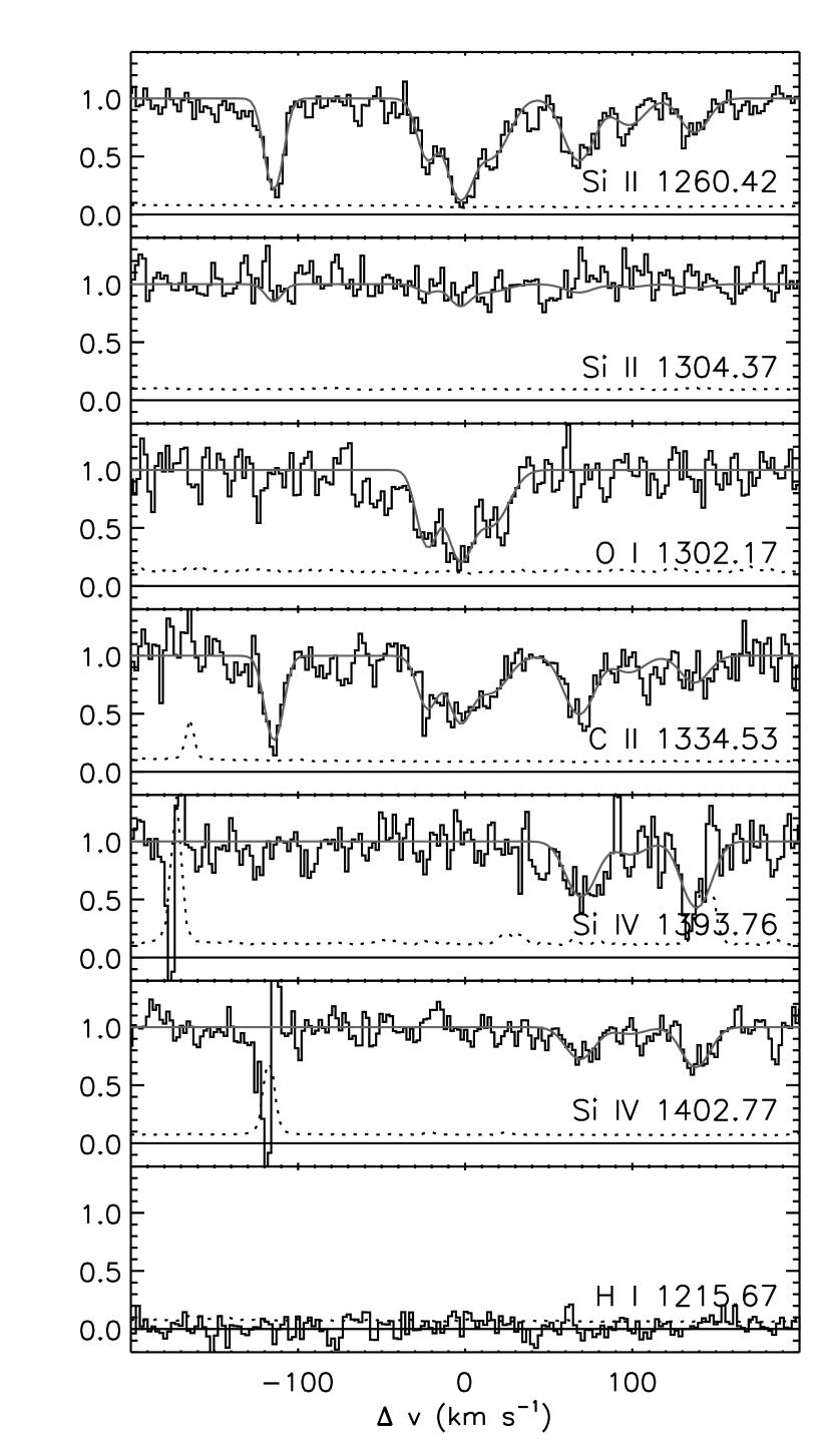
Figure 1: Absorption lines for the $z_{\rm sys}=5.3364$ O i system towards SDSS J0231$-$0728. Regions of the spectrum covering individual transitions have been shifted onto a common velocity scale. The histogram shows the normalized flux. The solid line shows the best Voigt profile fit. The dotted line shows the $1\sigma$ flux error.

3.1.1 SDSS J0231$-$0728: $z_{\rm sys}=5.3364$ (Figure 1)

This system shows a central complex in O i, Si ii, and C ii that is best fit using three components with a total velocity span of $\Delta v\approx 38$ km s^-1. We measure the redshifts and $b$-parameters of the bluest two central components from Si ii. The redshift and $b$-parameter for the reddest central component are measured from O i, which is least affected by additional lines towards the red. Leaving all parameters untied produces a two-component fit for C ii, which is likely due to low $S/N$. However, the total column densities remain virtually unchanged.

A single component at $\Delta v\approx-115$ km s^-1 appears in Si ii and C ii but not in O i. Since O i is more easily ionized than either Si ii or C ii ($\Delta E_{{\rm O\;\mbox{\tiny I}}}=13.6$ eV, $\Delta E_{{\rm Si\;\mbox{\tiny II}}}=16.3$ eV, $\Delta E_{{\rm C\;\mbox{\tiny II}}}=24.4$ eV) this component probably arises from gas that is more highly ionized than the gas producing the O i absorption. Three additional components appear redward of the central O i complex. These are visible in Si ii, C ii, and Si iv  and presumably correspond to gas in a still higher ionization state. We use Si ii to constrain the redshift and $b$-parameters for all the non-O i components, although fitting without tying any parameters produces very similar results.

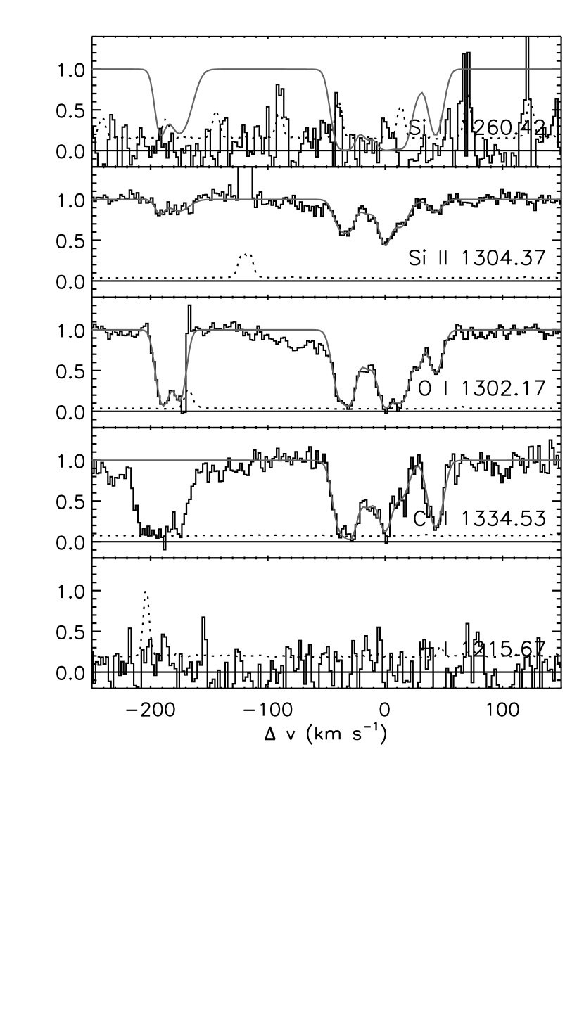
Figure 2: Absorption lines for the $z_{\rm sys}=5.8408$ O i system towards SDSS 1623+3112. See Figure 1 for details. The sharp features around Si ii $\lambda 1260$ are noise in the Ly$\alpha$ forest. The components at $\Delta v\approx-180$ km s^-1 are unconfirmed due to the strong $z_{\rm abs}=2.1979$ Mg i absorption at the wavelength where we would expect to see C ii.

3.1.2 SDSS J1623+3112: $z_{\rm sys}=5.8408$ (Figure 2)

This system shows multiple components with a total velocity span of $\Delta v\approx 81$ km s^-1. The Si ii is strong enough that the 1304 Å transition is clearly visible. Some additional absorption occurs along the blue edge of the O i complex. However, since no corresponding absorption appears in C ii this features is unlikely to be genuine O i. We use C ii to fix the redshifts and $b$-parameters of the bluest two components and the reddest component for all ions. The $z$ and $b$ values for the remaining components are tied to O i. The weakest C ii component was automatically dropped by the fitting program. However, this should not have a significant impact on the summed C ii column density. No Si iv was detected down to $N_{{\rm Si\;\mbox{\tiny IV}}}>10^{13}~{}{\rm cm^{-2}}$.

A strong line appears at a velocity separation $\Delta v\approx-180$ km s^-1 from the O i complex. Weak absorption appears at the same velocity in Si ii $\lambda 1304$. However, the corresponding C ii region is completely covered by Mg i $\lambda 2853$ from a strong Mg ii system at $z_{\rm abs}=2.1979$. Therefore, while these features are plausibly associated with the O i complex, their identity cannot presently be confirmed. We do not include these lines when computing the relative abundances, although their O i/Si ii ratio is consistent with those measured for the other O i systems.

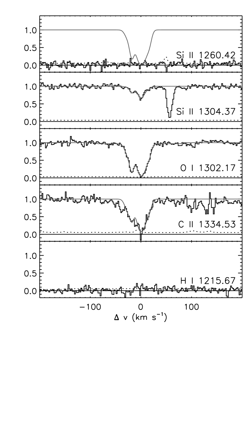
Figure 3: Absorption lines for the $z_{\rm sys}=6.0097$ O i system towards SDSS 1148+5251. See Figure 1 for details. Si ii $\lambda 1260$ falls in the Ly$\alpha$ forest. The strong line at $\Delta v=57$ km s^-1 from Si ii $\lambda 1304$ is Si ii $\lambda 1260$ at $z=6.2555$. The absorption features at $\Delta v\approx-40$ km s^-1 and $\Delta v\approx 90-140$ km s^-1 from C ii are probably telluric absorption that has not been fully removed.

3.1.3 SDSS J1148+5251: $z_{\rm sys}=6.0097$ (Figure 3)

This system shows multiple components with a velocity span of $\Delta v\approx 41$ km s^-1. The Si ii $\lambda 1260$ transition falls in the Ly$\alpha$ forest. However, Si ii $\lambda 1304$ is clearly visible. The C ii occurs among moderate-strength telluric absorption. In correcting for the atmosphere we recovered a C ii velocity profile very similar to that of O i and Si ii. Some additional absorption around the C ii are probably telluric lines that were not completely removed. We achieved the best fit for O i using four components while allowing the continuum level to vary slightly. Using fewer components resulted in virtually the same total $N_{{\rm O\;\mbox{\tiny I}}}$, which is to be expected if the lines lie along the linear part of the curve of growth. We used the $z$ and $b$ values for these four O i lines to determine the corresponding column densities for Si ii and C ii. Leaving all parameters untied resulted in small changes in the $b$-parameters and in the preferred number of lines used by VPFIT (3 for Si ii instead of 4), but negligible changes in the total column density for each ion. We detect no Si iv down to $N_{{\rm Si\;\mbox{\tiny IV}}}>10^{12.5}~{}{\rm cm^{-2}}$. This system does show C iv absorption in the low-resolution NIRSPEC spectrum taken by Barth et al. (2003). However, the kinematic structure cannot be determined from their data, and it is therefore unknown whether the C iv absorption arises from the same gas that produces the lower-ionization lines.

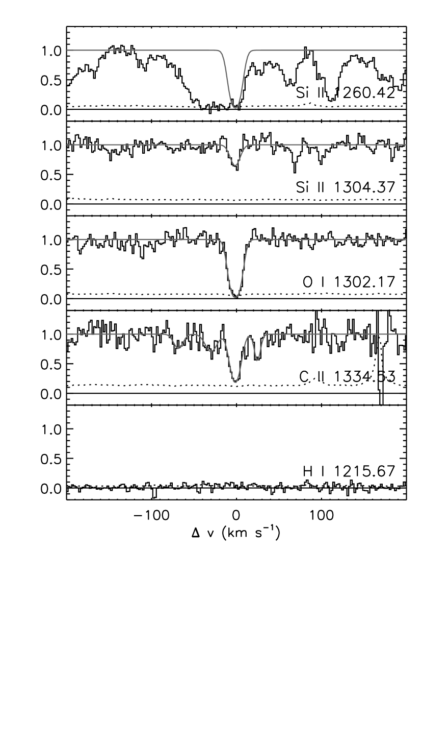
Figure 4: Absorption lines for the $z_{\rm sys}=6.1293$ O i system towards SDSS 1148+5251. See Figure 1 for details. The features around Si ii $\lambda 1260$ are Ly$\alpha$ absorption in the quasar proximity region. The C ii components at $\Delta v=-67,-29$ and 26 km s^-1 are unconfirmed.

3.1.4 SDSS J1148+5251: $z_{\rm sys}=6.1293$ (Figure 4)

The Si ii $\lambda 1260$ line for this system falls in the Ly$\alpha$ forest. However, Si ii $\lambda 1304$ is strong enough to be visible. We tie the redshifts and $b$-parameters for Si ii and C ii at $z=6.129267$ to those for O i, which has the cleanest profile. Leaving all parameters untied produces changes in the $b$-parameters that are within the errors and negligible changes in the column densities. Possible additional C ii lines appear at $\Delta v=-67$, -29, and 26 km s^-1 from the strong component. These do not appear in O i and would probably be too weak to appear in Si ii $\lambda 1304$. We do not include them when computing the relative abundances for this system. No Si iv was detected down to $N_{{\rm Si\;\mbox{\tiny IV}}}>10^{12.7}~{}{\rm cm^{-2}}$.

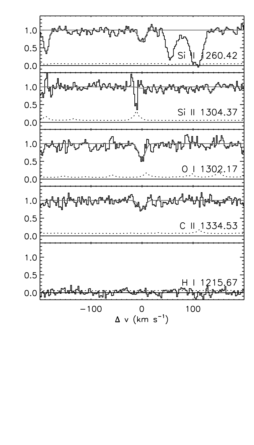
Figure 5: Absorption lines for the $z_{\rm sys}=6.1968$ O i system towards SDSS 1148+5251. See Figure 1 for details. The features near Si ii $\lambda 1260$ are unrelated metal lines. The sharp feature near Si ii $\lambda 1304$ is the residual from a strong skyline.

3.1.5 SDSS J1148+5251: $z_{\rm sys}=6.1968$ (Figure 5)

The Si ii $\lambda 1260$ and C ii lines for this system occur in transparent gaps within regions of mild telluric absorption. In some of our exposures, the O i line falls on the blue wing of a strong telluric feature. However, the O i can be clearly seen in the uncorrected 2005 January data, where the heliocentric velocity shifted the observed QSO spectrum further to the blue. We tie the redshifts and $b$-values for O i and C ii to those of Si ii, for which the line profile is the cleanest. Leaving all parameters untied produces negligible changes in the column densities.

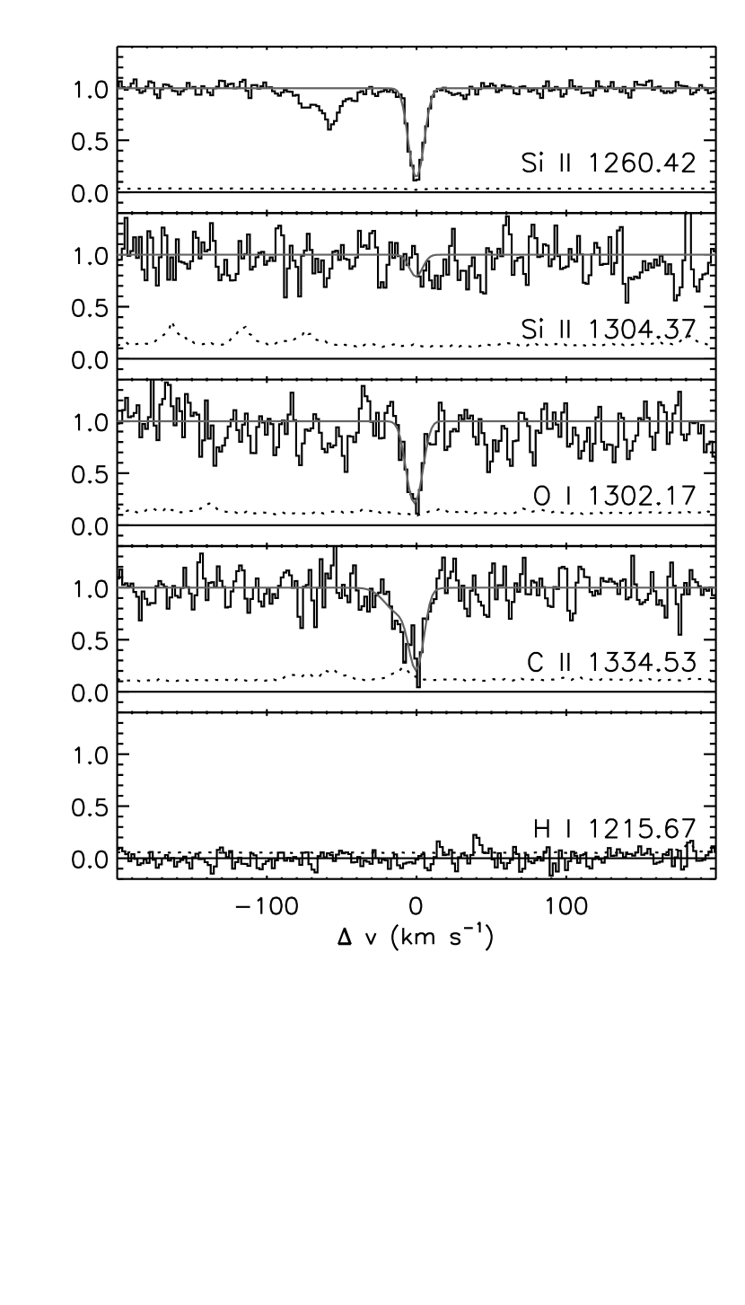
Figure 6: Absorption lines for the $z_{\rm sys}=6.2555$ O i system towards SDSS 1148+5251. See Figure 1 for details. The absorption at $\Delta v\approx-60$ km s^-1 from Si ii $\lambda 1260$ is Si ii $\lambda 1304$ at $z=6.0097$. The C ii fit includes an unconfirmed component on the blue edge of the profile.

3.1.6 SDSS J1148+5251: $z_{\rm sys}=6.2555$ (Figure 6)

We use a single component for the primary fit to this system. The C ii falls on a sky emission line and hence the line profile is rather noisy. We therefore tied the redshift and $b$-parameter for C ii to those of Si ii, while $z$ and $b$ for O i were allowed to vary freely. The fitted $z$ and $b$ values for O i agree with those for Si ii within the fit errors. Tying $z$ and $b$ for O i to those of Si ii produced no significant change in $N_{{\rm O\;\mbox{\tiny I}}}$. Both Si ii $\lambda 1260$ and O i are well fit by a single line, while the blue edge of the C ii shows a possible additional component. We fit this component separately but do include it when computing relative abundances.

4 Overabundance of O i systems towards SDSS J1148+5251

Despite the relatively small total number of detected O i systems, a noticable overabundance appears towards SDSS J1148+5251. It should be noted that this object has one of the brightest continuum magnitudes among QSOs at $z>5$ (Fan et al., 2003). We also spent considerable integration time on this object. Therefore, the data are among the best in our sample. In this section we address the null hypothesis that the apparent imbalance in the distribution of O i systems results from a combination of incompleteness and small number statistics.

For each sightline we used an automated scheme to determine the absorption pathlength interval $\Delta X$ over which we are sensitive to systems above a given O i column density. For a non-evolving population of sources expanding with the Hubble flow, we expect to intersect the same number of sources per unit $X$ at all redshifts, where $X$ is defined for $\Omega=1$ as

$$dX=\frac{(1+z)^{2}}{\sqrt{\Omega_{\rm m}(1+z)^{3}+\Omega_{\Lambda}}}dz\,.$$ (2)

At the redshift of each pixel where we are potentially sensitive to O i, we inserted artificial single-component systems containing O i, Si ii, and C ii with relative abundances set to the mean measured values (see §5) and a turbulent Doppler width of $b=10$ km s^-1. The minimum $N_{{\rm O\;\mbox{\tiny I}}}$ at which the system could be detected by the automated program was then determined. A detection required that there be significant ($4\sigma$) absorption at the expected wavelengths of O i and at least one of the other two ions. The redshifts of at least two of the three fitted profiles must also agree within a tolerance of $\Delta z_{tol}=0.0002$, and the line widths must agree to within a factor of two. In the case where the fitted profiles agree for only two of the ions, the spectrum at the wavelength of the third ion must be consistent with the expected level of absorption. This allows for one of the ions to be blended with another line or lost in Ly$\alpha$ forest. Lines that fell in the Fraunhofer A band were not considered. This method detected all of the known O i systems and produced only one false detection in the real data, which was easily dismissed by visual inspection. We note that this method focuses on our ability to detect systems similar to those observed towards SDSS J1148+5251. Multiple-component systems such as the two at lower redshift are in general easy to identify, even in noisy regions of the spectrum.

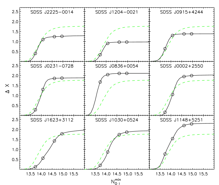
Figure 9: Sensitivity curves for each of our sightlines. The solid lines give the absorption pathlength interval over which we are sensitive to single-component O i systems with $N_{{\rm O\;\mbox{\tiny I}}}\geq N_{{\rm O\;\mbox{\tiny I}}}^{\rm min}$ and relative abundances similar to those of the O i systems in our sample. Circles mark the $\Delta X$ values corresponding to the $N_{{\rm O\;\mbox{\tiny I}}}$ of systems detected towards SDSS 1148+5251. The dashed line shows the mean $\Delta X$ as a function of $N_{{\rm O\;\mbox{\tiny I}}}^{\rm min}$ for all nine sightlines. The three lowest-redshift sightlines have smaller maximum $\Delta X$ values due in part to $A$-band atmospheric absorption.

The results of the sensitivity measurements are shown in Figure 9. The solid lines show the $\Delta X$ over which we are sensitive to systems with $N_{{\rm O\;\mbox{\tiny I}}}\geq N_{{\rm O\;\mbox{\tiny I}}}^{\rm min}$. The O i column densities for the four systems seen towards SDSS J1148+5251 are marked with circles. The dashed line shows the mean $\Delta X$ as a function of $N_{{\rm O\;\mbox{\tiny I}}}^{\rm min}$ for all nine sightlines. While it is clear that the path length over which we are sensitive to low-column density systems is considerably smaller for some sightlines than for SDSS J1148+5251, there does exist significant coverage across the total sample even at the $N_{{\rm O\;\mbox{\tiny I}}}$ of the weakest system in our sample.

Completeness effects will depend on the intrinsic distribution of line strengths, in that weaker systems will more easily be lost in low-$S/N$ sightlines. It is useful to define an effective absorption pathlength interval $\Delta X^{\rm eff}$ such that, for a sightline with a total pathlength $\Delta X^{\rm tot}$ and sensitivity $S(N)$, we would expect to detect the same number $\mathcal{N}$ of systems with $N\geq N_{\rm min}$ over $\Delta X^{\rm eff}$ if we had perfect sensitivity. For a column-density distribution $f(N)=\partial^{2}\mathcal{N}/\partial N\partial X$, this gives

$$\Delta X^{\rm eff}\int_{N_{\rm min}}^{\infty}{f(N)\,dN}=\Delta X^{\rm tot}\int_{N_{\rm min}}^{\infty}{f(N)\,S(N)\,dN}\,,$$ (3)

where $S(N)$ is the fraction of the total pathlength over which we are sensitive to systems with column density $N$. The sensitivity function can be determined directly from Figure 9. We assume a conventional power-law distribution in O i column densities $f(N_{{\rm O\;\mbox{\tiny I}}})\propto N_{{\rm O\;\mbox{\tiny I}}}^{-\alpha}$. Hence,

$$\Delta X^{\rm eff}=\Delta X^{\rm tot}\,\frac{\int_{N_{\rm min}}^{\infty}{N^{-\alpha}\,S(N)\,dN}}{\int_{N_{\rm min}}^{\infty}{N^{-\alpha}\,dN}}\,.$$ (4)

Taking into account our measured sensitivity, the maximum likelihood estimator for $\alpha$ for all six O i systems is $\hat{\alpha}=1.7$. A K-S test allows $1.3\leq\alpha\leq 2.1$ at the 95% confidence level.

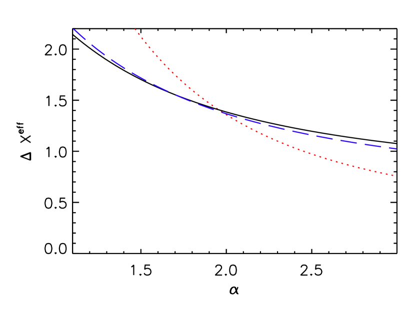
Figure 10: Effective absorption pathlength interval over which we are sensitive to O i systems with $N_{{\rm O\;\mbox{\tiny I}}}\geq 10^{13.7}~{}{\rm cm^{-2}}$ as a function of $\alpha$, where $f(N_{{\rm O\;\mbox{\tiny I}}})\propto N_{{\rm O\;\mbox{\tiny I}}}^{-\alpha}$ (see Eq. 3). The solid line shows $\Delta X^{\rm eff}$ for SDSS J1148+5251. The dashed line shows the summed $\Delta X^{\rm eff}$ for the remaining eight sightlines, divided by 5.7 to match SDSS J1148+5251 at $\alpha=1.7$. The dotted line shows the combined $\Delta X^{\rm eff}$ for SDSS 1030+0524 and SDSS J1623+3112. For reasonable values of $\alpha$, the ratio of $\Delta X^{\rm eff}$ for SDSS J1148+5251 and the remaining eight sightlines is essentially constant. We would therefore expect to see roughly six times as many O i systems along the other eight sightlines as towards SDSS J1148+5251 for a non-evolving population of absorbers.

In Figure 10 we plot $\Delta X^{\rm eff}$ as a function of $\alpha$ taking $N_{\rm min}=10^{13.7}$ cm^-2 as the cutoff value. The solid line shows $\Delta X^{\rm eff}$ for SDSS J1148+5251, while the dashed line shows $\Delta X^{\rm eff}$ for the remaining eight sightlines, divided by 5.7 to match SDSS J1148+5251 at $\alpha=1.7$. It is easy to see that the ratio $\Delta X^{\rm eff}_{1148}/\Delta X^{\rm eff}_{\rm other}$ does not change significantly with $\alpha$ ($\lesssim 4\%$ over $1.1\leq\alpha\leq 3.0$). This is purely a coincidence, most likely related to the fact that the overall high quality of the SDSS J1148+5251 data is balanced by the placement of the O i systems in a difficult region of the spectrum. However, it means that the relative numbers of expected O i detections for SDSS J1148+5251 and the remaining eight sightlines should be nearly invariant over a wide range in plausible column density distributions.

We can now evaluate the likelihood that the imbalance of O i detection results from small number sampling. For a Poisson distribution, the likelihood of detecting $\mathcal{N}$ systems when the expected number of detections is $\nu$ is given by

$$P(\mathcal{N},\nu)=\frac{\nu^{\,\mathcal{N}}e^{-\nu}}{\mathcal{N}}\,.$$ (5)

If we assume that the expected number of detections towards SDSS J1148+5251 is $\nu=6\,(\Delta X^{\rm eff}_{1148}/\Delta X^{\rm eff}_{\rm all})\simeq 0.90$, then the probability of detecting at least 4 systems is

$$P(\geq 4,\nu)=\sum_{\mathcal{N}=4}^{\infty}{P(\mathcal{N},\nu)}=1-\sum_{\mathcal{N}=0}^{3}{P(\mathcal{N},\nu)}=0.013\,.$$ (6)

Similarly, if we take the number of systems observed towards SDSS J1148+5251 as a representative sample and compute the expected number of systems towards the remaining eight sightlines to be $\nu=4\,(\Delta X^{\rm eff}_{\rm other}/\Delta X^{\rm eff}_{1148})\simeq 23$, then the likelihood of detecting at most two systems is

$$P(\leq 2,\nu)=\sum_{\mathcal{N}=0}^{2}{P(\mathcal{N},\nu)}=3.6\times 10^{-8}\,.$$ (7)

The probability of simultaneously detecting at least 4 systems towards SDSS J1148+5251 while detecting at most two systems along the remaining eight sightlines,

$$P\left(\frac{\partial\mathcal{N}}{\partial X}\right)=\left[1-\sum_{\mathcal{N}=0}^{3}{P(\mathcal{N},\frac{\partial\mathcal{N}}{\partial X}\,\Delta X^{\rm eff}_{1148})}\right]\,\left[\sum_{\mathcal{N}=0}^{2}{P(\mathcal{N},\frac{\partial\mathcal{N}}{\partial X}\,\Delta X^{\rm eff}_{\rm other})}\right]\,,$$ (8)

has a maximum of $P(\partial\mathcal{N}/\partial X)=0.0018$ at $\partial\mathcal{N}/\partial X=0.84$, taking $\alpha\leq 3$. Thus, assuming that the O i systems are randomly distributed, we can rule out with a high degree of confidence the possibility that the excess number of detected systems towards SDSS J1148+5251 is the result of a statistical fluctuation.

4.1 Comparison with Lower-Redshift Sightlines

Our sample of nine $z_{\rm QSO}>4.8$ sightlines is sufficient to demonstrate that the apparent excess of O i systems towards SDSS 1148+5251 is highly unlikely to arise from a random spatial distribution of absorbers. However, the distribution may be significantly non-random due to large-scale clustering. For example, if the line-of-sight towards SDSS 1148+5251 passes through an overdense region of the IGM then we might expect to intersect more than the typical number of absorbers.

To address this possibility, we have searched for O i in the spectra of an additional 30 QSOs with $2.6<z_{\rm QSO}<4.6$. The sample was taken entirely with HIRES for a variety of studies. Due to the lower QSO redshifts, the data are of significantly higher quality than the $z_{\rm QSO}>4.8$ sample. All sightlines are complete down to $N_{{\rm O\;\mbox{\tiny I}}}=10^{13.5}~{}{\rm cm^{-2}}$ (apart from rare wavelength coverage gaps) with the majority complete down to $N_{{\rm O\;\mbox{\tiny I}}}=10^{13.0}~{}{\rm cm^{-2}}$.

A detailed study of the properties of lower-redshift O i absorbers will be presented elsewhere. Here we note that 11 systems with $N_{{\rm O\;\mbox{\tiny I}}}>10^{13.7}~{}{\rm cm^{-2}}$ were identified along all 30 sightlines in the redshift intervals where O i would occur redward of the Ly$\alpha$ forest. This is comparable to but slightly larger than the incidence rate among the eight lowest-redshift sightlines in our $z_{\rm QSO}>4.8$ sample. The number density is even somewhat higher among the $z_{\rm QSO}<4.6$ sample since the absorption pathlength intervals are shorter (cf. Eq. 2). However, many of the $z_{\rm QSO}<4.6$ spectra were taken in order to study known damped Ly$\alpha$ systems (DLAs; $N_{{\rm H\;\mbox{\tiny I}}}>10^{20.3}~{}{\rm cm^{-2}}$), which commonly exhibit O i (e.g., Prochaska et al., 2001, 2003). We would therefore expect these sightlines to contain more than the typical number of O i systems. The important point is that no sightline contained more than a single system. If the excess towards SDSS J1148+5251 is due to the chance alignment with an overdense region of the IGM, then such a coincidence must occur in fewer than $\sim 2-3\%$ of all sightlines.

4.2 Comparison with Damped Ly$\alpha$ and Lyman Limit System Populations

We can compare the observed number of O i systems in our $z_{\rm QSO}>4.8$ sample with the expected number of DLAs by extrapolating from lower-redshift DLA surveys. Storrie-Lombardi & Wolfe (2000) find a line number density $n_{\rm DLA}(z)=\partial\mathcal{N}_{\rm DLA}/\partial z=0.055\,(1+z)^{1.11}$. This is consistent at high-$z$ with the larger survey done by Prochaska et al. (2005) and with the number density evolution Rao et al. (2005) obtained by combining DLA samples over $0\leq z\leq 4.5$. From this $n_{\rm DLA}(z)$ we would expect a total of $\sim 1.5$ DLAs total along all nine lines-of-sight in the redshift intervals where are sensitive to O i. This is consistent with the two O i systems seen along the eight lower-redshift sightlines. However, we would expect to see only $\sim 0.2$ DLAs towards SDSS J1148+5251, which is inconsistent with the four we observe.

The disparity eases for SDSS J1148+5251 if we include all Lyman limit Systems (LLSs; $N_{{\rm H\;\mbox{\tiny I}}}>10^{17.2}~{}{\rm cm^{-2}}$). The line number density of LLSs at $z>2.4$ found by Péroux et al. (2003), $n_{\rm LLS}(z)=0.07\,(1+z)^{2.45}$, predicts $\sim 4$ LLSs towards SDSS J1148+5251 in the interval where we can observe O i. However, there should also be $\sim 20$ LLSs along the remaining eight lines-of-sight. If the excess O i absorbers are associated with the progenitors of lower-redshift LLSs then they must evolve strongly in O i at $z\gtrsim 6$.

5 Metal Abundances

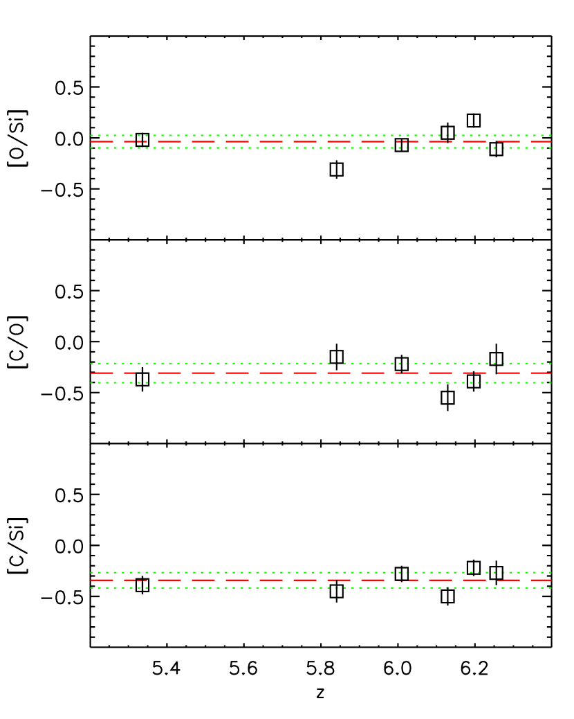
Figure 11: Relative metal abundances in the O i systems assuming no ionization corrections. Individual measurements plotted as squares with $1\sigma$ error bars are taken from Table 3. Dashed lines show the weighted mean values for all six systems. Dotted lines show the $2\sigma$ uncertainties in the means.

Absorption systems at $z>5$ provide an opportunity to study metal enrichment when the age of the Universe was $\lesssim 1$ Gyr. The opacity of the Ly$\alpha$ forest at these redshifts prevents us from measuring reliable H i column densities. However, we are still able to constrain relative abundances. In Table 3 we summarize the Voigt profile fitting results. Total column densities for each system include only components with confirmed O i. Relative abundances were calculated using the solar values of Grevesse & Sauval (1998) and assuming zero ionization corrections. These are plotted in Figure 11. The error-weighted mean values for all six systems are $\langle[{\rm O}/{\rm Si}]\rangle=-0.04\pm 0.06$, $\langle[{\rm C}/{\rm O}]\rangle=-0.31\pm 0.09$, and $\langle[{\rm C}/{\rm Si}]\rangle=-0.34\pm 0.07$ (2$\sigma$ errors).

The uncorrected abundances are broadly consistent with the expected yields from Type II supernovae of low-metallicity progenitors (Woosley & Weaver, 1995; Chieffi & Limongi, 2004). Low- and intermediate-mass stars should not contribute significantly to the enrichment of these systems since these stars will not have had time to evolve by $z\sim 6$ (although see Barth et al., 2003). We can use the O/Si ratio to constrain the enrichment from zero-metallicity very massive stars (VMSs, $M_{\star}\sim 140-270\,M_{\sun}$). VMSs exploding as pair instability supernovae are expected to yield $\sim 4$ times as much silicon compared to Type II SNe for the same amount of oxygen (Schaerer, 2002; Umeda & Nomoto, 2002; Heger & Woosley, 2002; Woosley & Weaver, 1995; Chieffi & Limongi, 2004). We can estimate the fraction $f^{\rm VMS}_{\rm Si}$ of silicon contributed by VMSs to these systems using the simple mixing scheme of Qian & Wasserburg (2005a, b),

$$\left(\frac{\rm O}{\rm Si}\right)=\left(\frac{\rm O}{\rm Si}\right)_{\rm VMS}f_{\rm Si}^{\rm VMS}+\left(\frac{\rm O}{\rm Si}\right)_{\rm SN\,II}\left(1-f_{\rm Si}^{\rm VMS}\right)\,.$$ (9)

Adopting ${\rm[O/Si]_{\rm VMS}}=-0.61$ from Heger & Woosley (2002), and ${\rm[O/Si]_{\rm SN\,II}}=0.00$ from Woosley & Weaver (1995), the mean uncorrected O/Si gives $f^{\rm VMS}_{\rm Si}=0.11\pm 0.17~{}(2\sigma)$. However, this value of O/Si should be considered a lower limit. The ionization potential of O i is smaller than that of Si ii ($\Delta E_{{\rm O\;\mbox{\tiny I}}}=13.6$ eV, $\Delta E_{{\rm Si\;\mbox{\tiny II}}}=16.3$ eV). Therefore, applying an ionization correction would increase O/Si. Taking $\langle[{\rm O}/{\rm Si}]\rangle>-0.10$ gives $f^{\rm VMS}_{\rm Si}<0.27~{}(2\sigma)$.

The mean C/Si ratio is consistent with zero silicon contribution from VMSs, although C/Si may decrease if ionization corrections are applied ($\Delta E_{{\rm C\;\mbox{\tiny II}}}=24.4$ eV $>\Delta E_{{\rm Si\;\mbox{\tiny II}}}$). Dust corrections would also decrease C/Si since silicon is more readily depleted onto grains (Savage & Sembach, 1996). Our upper limit of $\langle[{\rm C}/{\rm Si}]\rangle<-0.27~{}(2\sigma)$ therefore does not provide an additional constraint on $f^{\rm VMS}_{\rm Si}$. However, the limit set by O/Si may still imply that VMSs provided a smaller fraction of the metals in these O i systems than in the general IGM. Qian & Wasserburg (2005a, b) have argued that VMSs at $z\gtrsim 15$ must have contributed $\gtrsim 50\%$ of the silicon in the IGM in order to produce ${\rm[Si/C]_{\rm IGM}}\sim 0.7$ at $z\approx 2-4$ (Aguirre et al., 2004). However, the Si/C ratio in the IGM derived from high-ionization lines depends sensitively on the choice of ionizing backgrounds.

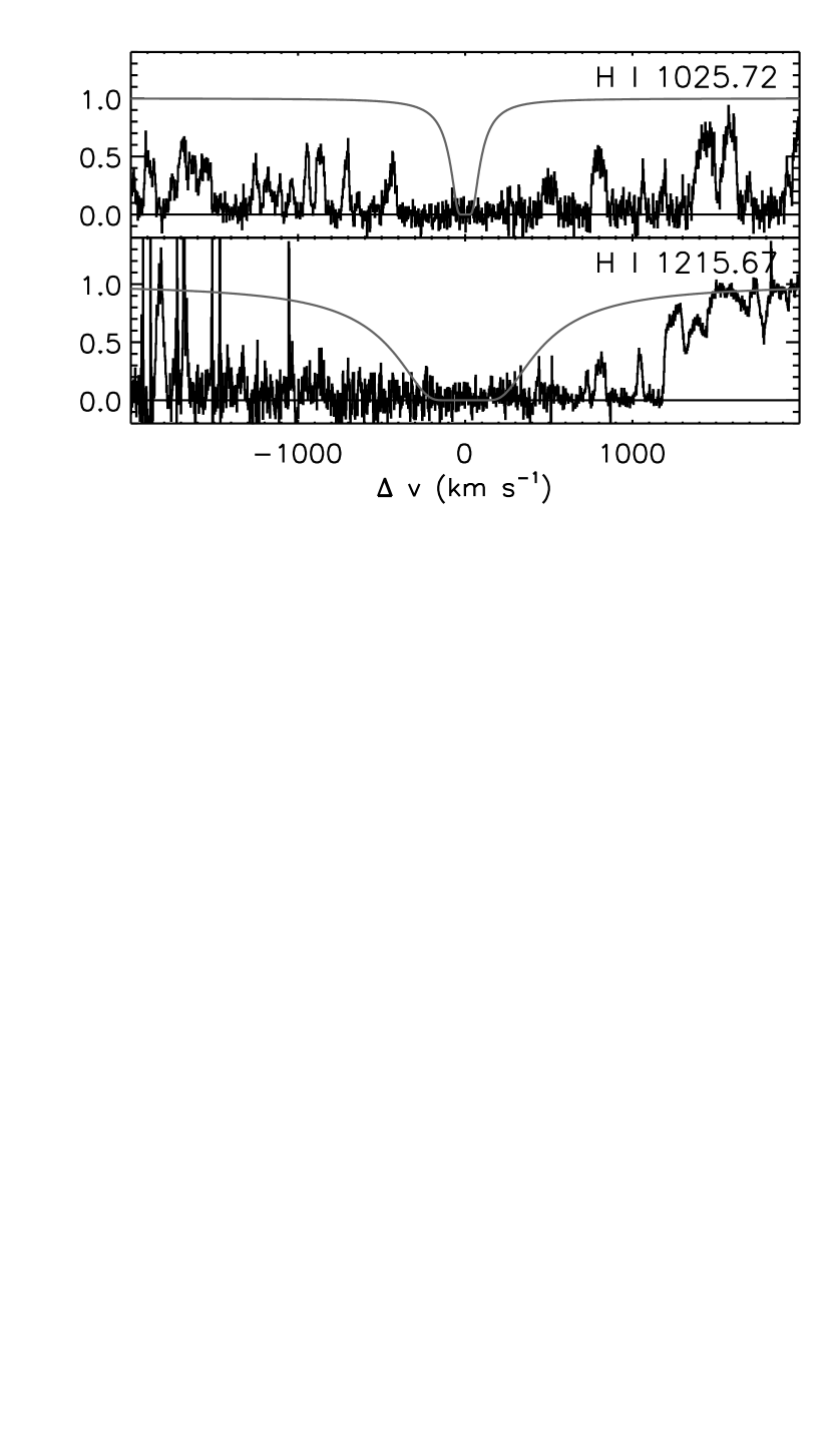
Figure 7: Voigt profile fit to H i Ly$\alpha$ and Ly$\beta$ corresponding to the upper limit on $N_{{\rm H\;\mbox{\tiny I}}}$ for the $z_{\rm sys}=5.3364$ O i systems towards SDSS J0231$-$0728. In order to set an upper limit on $N_{{\rm H\;\mbox{\tiny I}}}$ we have taken $b=1$ km s^-1, although the actual $b$-parameter is likely to be significantly larger. In this system, $N_{{\rm H\;\mbox{\tiny I}}}$ is constrained by the transmitted flux in the wings of the Ly$\alpha$ profile.

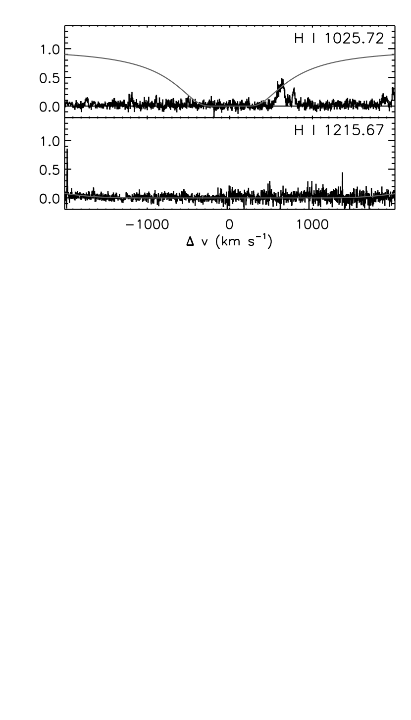
Figure 8: Voigt profile fit to H i Ly$\alpha$ and Ly$\beta$ corresponding to the upper limit on $N_{{\rm H\;\mbox{\tiny I}}}$ for the $z_{\rm sys}=6.0097$ O i systems towards SDSS J1148+5251. In this system, $N_{{\rm H\;\mbox{\tiny I}}}$ is constrained by the transmitted flux in the red wing of the Ly$\beta$ profile.

The high level of absorption blueward of the Ly$\alpha$ emission line at $z>5$ prevents us from reliably fitting Voigt profiles to H i. However, transmission peaks in the Ly$\alpha$ and Ly$\beta$ forests near the O i redshifts allow us to set upper limits on the H i column density for two of our systems. Fits to these systems with the strongest allowable damping wings are shown in Figures 7 and 8, and the corresponding limits are listed in Table 3. The limits take into account uncertainties in the continuum level, which was set to a power-law $F_{\nu}\propto\lambda^{-\beta}$ with spectral index $\beta=0.5$, normalized at a rest wavelength of 1280 Å. The continuum uncertainty will include the error in the amplitude of the power law at the wavelength of the damped system. Taking $\Delta\beta=0.65$ to incorporate 95% of the scatter in QSO spectral indices (Richards et al., 2001), this error is $<10\%$ for the system at $z_{\rm sys}=5.3364$, for which the limit on $N_{{\rm H\;\mbox{\tiny I}}}$ was set using Ly$\alpha$ transmission, and $<20\%$ for the system at $z_{\rm sys}=6.0097$, for which the limit was set using Ly$\beta$. Larger uncertainties in the continuum may result from errors in the relative flux calibration and the departure from a power law. We conservatively estimate both of these to be $\sim 20\%$, which translates to an uncertainty in the column density $\sigma(\log{N_{{\rm H\;\mbox{\tiny I}}}})\sim 0.3$. The upper limits on $\log{N_{{\rm H\;\mbox{\tiny I}}}}$ listed in Table 3 are our “best fit” values plus this uncertainty. The corresponding limits on the absolute abundances are $[{\rm O}/{\rm H}]>-2.4$ ($z_{\rm sys}=5.3364$) and $[{\rm O}/{\rm H}]>-4.1$ ($z_{\rm sys}=6.0097$).

The comoving mass density for each ion is given by

$$\Omega_{\rm ion}=\frac{H_{0}m_{\rm ion}}{c\rho_{\rm crit}}\frac{\sum{N_{\rm ion}}}{\Delta X^{\rm tot}}\,,$$ (10)

where $m_{\rm ion}$ is the mass of the ion, $\rho_{\rm crit}=0.92\times 10^{-29}~{}h_{70}^{2}~{}{\rm g~{}cm^{-3}}$ is the cosmological closure density, and $\Delta X^{\rm tot}$ is the total pathlength interval over which we are sensitive to O i. In Table 4 we list $\Omega_{\rm ion}$ for O i, Si ii, and C ii summing over all $z_{\rm QSO}>4.8$ sightlines, over the three sightlines with $z_{\rm QSO}>6.2$ only, and over the sightline towards SDSS J1148+5251 only. The mass densities include all confirmed absorption components, including those without detected O i. However, we have made no attempt to correct for incompleteness. The densities of low-ionization metal species along our $z_{\rm QSO}>6.2$ sightlines are comparable to the densities of the corresponding high-ionization species at lower-redshift. Songaila (2005) measured $\Omega(\mbox{C~{}{\sc iv}})\sim 3\times 10^{-8}$ and $\Omega(\mbox{Si~{}{\sc iv}})\sim 1\times 10^{-8}$ over $1.5<z<4.5$, with a drop in $\Omega(\mbox{C~{}{\sc iv}})$ by at least a factor of two at $z>5$. A decrease in high-ionization metals and a correlated rise in their low-ionization counterparts with redshift might signal a change in the ionization state of the $z>5$ IGM. However, coverage of C iv does not currently extend to $z\sim 6$, and our O i sample is probably too small to make a meaningful comparison.

6 Discussion

Although we observe an overabundance of O i at $z>6$ along one of our highest-redshift sightlines, it is not clear that these four systems constitute a “forest” which would signal a predominantly neutral IGM. In the reionization phase prior to the overlap of ionized bubbles, Oh (2002) predicts tens to hundreds of O i lines with $N_{{\rm O\;\mbox{\tiny I}}}>10^{14}~{}{\rm cm^{-2}}$, although the number may be lower if the enriched regions have very low metallicity ($Z<10^{-2.5}Z_{\sun}$), or if the volume filling factor of metals is small ($f_{Z}\ll 0.01$). The number of O i systems we detect is more consistent with his predictions for the post-overlap phase, although the expected number of lines depends on the ionizing efficiency of the metal-producing galaxies. The Oh (2002) model also predicts lines with $N_{{\rm O\;\mbox{\tiny I}}}>10^{15}~{}{\rm cm^{-2}}$, which we do not observe.

The significance of the excess O i towards SDSS J1148+5251 is complicated by the presence of Ly$\alpha$ and Ly$\beta$ transmission along that sightline. The O i systems occur interspersed in redshift with the Ly$\beta$ peaks, with the velocity separation from the nearest peak ranging from $\Delta v\sim 500$ to $3000$ km s^-1 ($\Delta l\sim 5$ to $30$ comoving Mpc). The O i absorbers also do not appear to be clustered. Along a total redshift interval $\Delta z_{\rm tot}=0.49$ ($\sim 200$ comoving Mpc) where we are sensitive to O i, the detected systems are separated by $\Delta z=0.06$ to $0.12$ ($\Delta l=24$ to $50$ comoving Mpc). If any significantly neutral regions are present along this sightline, then they occur within or near regions that are highly ionized. In contrast, we find no O i towards SDSS J1030+0524, despite the fact that its spectrum shows complete absorption in Ly$\alpha$ and Ly$\beta$ over $\Delta z\sim 0.2$. The SDSS J1030+0524 sightline may pass through a region of the IGM that is still largely neutral and not yet enriched. Alternatively, there may be no O i because the sightline is highly ionized. In that case, a large-scale density enhancement could still produce the high Ly$\alpha$ and Ly$\beta$ optical depth (Wyithe & Loeb, 2005).

The overabundance of O i together with the transmission in Ly$\alpha$ and Ly$\beta$ indicates that the SDSS J1148+5251 sightline has experienced both significant enrichment and ionization. One explanation is that we are looking along a filament. The total comoving distance between O i systems towards SDSS J1148+5251 is $\approx 101$ Mpc, which is smaller than the largest known filamentary structures at low redshift (e.g., Gott et al., 2005). If the line-of-sight towards SDSS 1148+5251 runs along a filament at $z\sim 6$ then we might expect to intersect more than the average number of absorbers. Galaxies along such a structure might produce enough ionizing radiation to create the transmission gaps observed in the Ly$\alpha$ and Ly$\beta$ forests while still allowing pockets of neutral material to persist if the ionizing background is sufficiently low. If we assume that every $z\sim 6$ galaxy is surrounded by an enriched halo, then we can calculate the typical halo radius

$$R_{\rm halo} \sim \left[\frac{\mathcal{N}}{\pi(1+z)^{2}\left<\Phi_{\rm gal}\right>\delta_{\rm gal}\Delta D}\right]^{1/2}$$ (12)

$$\sim 35~{}{\rm proper~{}kpc}\,\left(\frac{\mathcal{N}}{4}\right)^{1/2}\left(\frac{1+z}{7.2}\right)^{-1}\left(\frac{\left<\Phi_{\rm gal}\right>}{0.01\,{\rm Mpc^{-3}}}\right)^{-1/2}$$

$$\times\left(\frac{\delta_{\rm gal}}{10}\right)^{-1/2}\left(\frac{\Delta D}{200\,{\rm Mpc}}\right)^{-1/2}\,.$$

Here, $\Delta D$ is the total comoving distance over which we are sensitive to O i. We have used the mean comoving number of galaxies $\left<\Phi_{\rm gal}\right>$ at $z\sim 6$ measured down to the limit of the Hubble Ultra Deep Field (UDF; Yan & Windhorst, 2004; Bouwens et al., 2005), and assumed an overdensity of galaxies $\delta_{\rm gal}=\Phi_{\rm gal}/\left<\Phi_{\rm gal}\right>=10$ along this sightline. The absorption could be due to filled halos, shells, or other structures surrounding the galaxies. Note that by inverting Eq. 12 we can rule out the possibility that these O i systems arise from the central star-forming regions of galaxies similar those observed in the UDF. The small size $R_{\rm half-light}\sim 0.8$ kpc of galaxies at $z\sim 6$ (Bouwens et al., 2005) would require either a local galaxy overdensity $\delta_{\rm gal}\sim 10^{4}$ or a large number of faint galaxies to produce the observed absorption systems.

At present we can place relatively few physical constraints on these absorbers. Assuming charge-exchange equilibrium (Eq. 1), we can estimate the H i column densities as a function of metallicity,

$$\log{N_{{\rm H\;\mbox{\tiny I}}}}=16.9+\log{\left(\frac{N_{{\rm O\;\mbox{\tiny I}}}}{10^{13.7}~{}{\rm cm^{-2}}}\right)}-\rm{[O/H]}\,.$$ (13)

For solar metallicities, even the weakest O i system in our sample must be nearly optically thick. Metal-poor absorbers with [O/H] $<-2$ would require column densities $N_{{\rm H\;\mbox{\tiny I}}}\gtrsim 10^{19}~{}{\rm cm^{-2}}$, which is consistent with the indication from the relative metal abundances that these absorbers are largely neutral.

Finally, the excess O i absorbers are distinguished by their small velocity dispersions. Three out of the four systems towards SDSS J1148+5251 have single components with Doppler widths $b\approx 5-8$ km s^-1. We may be seeing only the low-ionization component of a kinematically more complex structure such as a galactic outflow (e.g., Simcoe et al., 2005). However, if there are additional high-ionization components that would appear in C iv and Si iv then we might expect to see components in C ii and possibly Si ii without O i. This is the case in the $z_{\rm sys}=5.3364$ system towards SDSS J0231-0728. The $z_{\rm sys}=6.1293$ and $z_{\rm sys}=6.2550$ systems towards SDSS J1148+5251 show potential C ii lines that do not appear in O i, but these are relatively weak, and in the $z_{\rm sys}=6.1293$ system there is no apparent strong Si iv. Among the 11 O i absorbers in the $z<4.6$ sample, only three have a single O i component with a velocity width comparable to the three narrowest systems towards SDSS J1148+5251. The fact that the excess O i systems appear kinematically quiescent further suggests that they are a distinct class of absorbers.

7 Summary

We have conducted a search for O i in the high-resolution spectra of 9 QSOs at $4.8\leq z_{\rm QSO}\leq 6.4$. In total, we detect six systems in the redshift intervals where O i $\lambda 1302$ falls redward of the Ly$\alpha$ forest. Four of these lie towards SDSS J1148+5251 ($z_{\rm QSO}=6.42$). This imbalance is not easily explained by small number statics or by varying sensitivity among the data. A search at lower redshift revealed no more than than one O i system per sightline in a high-quality sample of 30 QSOs with $2.6\leq z_{\rm QSO}\leq 4.6$. The number of excess systems is significantly larger than the expected number of damped Ly$\alpha$ systems at $z\sim 6$, but similar to the predicted number of Lyman limit systems.

The six systems have mean relative abundances $\langle[{\rm O}/{\rm Si}]\rangle=-0.04\pm 0.06$, $\langle[{\rm C}/{\rm O}]\rangle=-0.31\pm 0.09$, and $\langle[{\rm C}/{\rm Si}]\rangle=-0.34\pm 0.07$ ($2\sigma$ errors), assuming no ionization corrections. These abundances are consistent with enrichment dominated by Type II supernovae. The lower limit on the oxygen to silicon ratio $\langle[{\rm O}/{\rm Si}]\rangle>-0.10$ is insensitive to ionization corrections and limits the contribution of silicon from VMSs to $<30\%$ in these systems. The upper limits on the ratio of carbon to oxygen ${\rm[C/O]}\leq-0.13$, and carbon to silicon ${\rm[C/Si]}\leq-0.20$ are also insensitive to ionization. Integrating over only the confirmed absorption lines, the mean ionic comoving mass densities along the three $z_{\rm QSO}>6.2$ sightlines are $\Omega_{{\rm O\;\mbox{\tiny I}}}\approx 7.0\times 10^{-8}$, $\Omega_{{\rm Si\;\mbox{\tiny II}}}\approx 9.6\times 10^{-9}$, and $\Omega_{{\rm C\;\mbox{\tiny II}}}\approx 1.5\times 10^{-8}$.

The excess O i systems towards SDSS J1148+5251 occur in redshift among Ly$\alpha$ and Ly$\beta$ transmission features, which indicates that the IGM along this sightline has experienced both enrichment and significant ionization. The sightline may pass along a filament, where galaxies are producing enough ionizing photons create the transmission gaps while still allowing a few neutral absorbers to persist. In contrast, no O i was observed towards SDSS J1030+0524, whose spectrum shows complete Gunn-Peterson absorption. The SDSS J1030+0524 sightline may pass through an underdense region containing very few sources that would either enrich or ionize the IGM. Alternatively, the sightline may be highly ionized, with a large-scale density enhancement producing strong line-blending in the Ly$\alpha$ and Ly$\beta$ forests. Future deep imaging of these fields and near-infrared spectroscopy covering high-ionization metal lines will allow us to distinguish between these scenarios and clarify the nature of the excess O i absorbers.

Table 1: Summary of Observations

QSO	$z_{\rm QSO}$	Dates	$\Delta t_{\exp}$ (hrs)
SDSS J2225$-$0014	4.87	2004 Jun	6.7
SDSS J1204$-$0021	5.09	2005 Jan - Feb	6.7
SDSS J0915$+$4244	5.20	2005 Jan - Feb	10.8
SDSS J0231$-$0728	5.42	2005 Jan - Feb	10.0
SDSS J0836$+$0054	5.80	2003 Feb - 2005 Jan	21.7
SDSS J0002$+$2550	5.82	2005 Jan - Jun	4.2
SDSS J1623$+$3112	6.22	2005 Jun	12.5
SDSS J1030$+$0524	6.30	2005 Feb	12.0
SDSS J1148$+$5251	6.42	2003 Feb - 2005 Feb	22.0

Table 2: Measured Properties of O i Systems

Ion	$z$	$b$ (km s-1)	$\log{N}~{}{\rm(cm^{-2})}$
SDSS J0231$-$0728: $z_{\rm sys}=5.3364$
Si ii	$5.333982\pm 0.000008$	$5.38\pm 0.58$	$12.786\pm 0.055$
C ii	$5.333982$	$5.38$	$13.584\pm 0.068$
Si ii	$5.335928\pm 0.000020$	$6.91\pm 1.33$	$12.514\pm 0.079$
Si ii	$5.336337\pm 0.000019$	$7.62\pm 1.60$	$12.978\pm 0.087$
Si ii	$5.336721$	$12.96$	$12.711\pm 0.135$
O i	$5.335928$	$6.91$	$13.982\pm 0.086$
O i	$5.336337$	$7.62$	$14.138\pm 0.129$
O i	$5.336721\pm 0.000072$	$12.96\pm 3.23$	$13.972\pm 0.143$
C ii	$5.335928$	$6.91$	$13.298\pm 0.077$
C ii	$5.336337$	$7.62$	$13.454\pm 0.119$
C ii	$5.336721$	$12.96$	$13.314\pm 0.138$
Si ii	$5.337841\pm 0.000014$	$10.89\pm 0.98$	$12.678\pm 0.040$
Si ii	$5.338474\pm 0.000043$	$11.71\pm 3.39$	$12.233\pm 0.098$
Si ii	$5.339301\pm 0.000016$	$10.44\pm 1.13$	$12.316\pm 0.063$
C ii	$5.337841$	$10.89$	$13.512\pm 0.051$
C ii	$5.338474$	$11.71$	$12.880\pm 0.161$
C ii	$5.339301$	$10.45$	$13.074\pm 0.097$
Si iv	$5.337841$	$10.89$	$12.848\pm 0.051$
Si iv	$5.338474$	$11.71$	$12.142\pm 0.192$
Si iv	$5.339301$	$10.44$	$12.950\pm 0.049$
SDSS J1623+3112: $z_{\rm sys}=5.8408$
O i	$5.836481\pm 0.000012$	$5.01\pm 0.59$	$14.376\pm 0.075$
O i	$5.836806\pm 0.000017$	$4.44\pm 1.57$	$14.216\pm 0.111$
Si ii	$5.836423\pm 0.000029$	$3.63\pm 2.66$	$12.746\pm 0.182$
Si ii	$5.836799\pm 0.000060$	$10.82\pm 4.29$	$12.985\pm 0.124$
Si ii	$5.839938$	$6.37$	$13.279\pm 0.182$
Si ii	$5.840138$	$4.13$	$13.063\pm 0.340$
Si ii	$5.840456$	$6.92$	$12.931\pm 0.196$
Si ii	$5.840798$	$5.32$	$13.488\pm 0.060$
Si ii	$5.841113$	$7.33$	$13.271\pm 0.078$
Si ii	$5.841456$	$1.77$	$11.655\pm 1.018$
Si ii	$5.841780$	$6.23$	$12.854\pm 0.070$
O i	$5.839938$	$6.37$	$14.214\pm 0.212$
O i	$5.840138$	$4.13$	$14.152\pm 0.242$
O i	$5.840456\pm 0.000032$	$6.92\pm 4.21$	$13.734\pm 0.206$
O i	$5.840798\pm 0.000014$	$5.32\pm 0.94$	$14.384\pm 0.084$
O i	$5.841113\pm 0.000025$	$7.33\pm 1.48$	$14.316\pm 0.073$
O i	$5.841456\pm 0.000014$	$1.77\pm 1.72$	$13.518\pm 0.150$
O i	$5.841780$	$6.23$	$13.793\pm 0.027$
C ii	$5.839938\pm 0.000055$	$6.37\pm 1.56$	$13.811\pm 0.231$
C ii	$5.840138\pm 0.000039$	$4.13\pm 2.50$	$13.955\pm 0.249$
C ii	$5.840456$	$6.92$	$13.431\pm 0.193$
C ii	$5.840798$	$5.32$	$13.771\pm 0.093$
C ii	$5.841113$	$7.33$	$13.316\pm 0.101$
C ii	$5.841780\pm 0.000007$	$6.23\pm 0.51$	$13.736\pm 0.055$
SDSS J1148+5251: $z_{\rm sys}=6.0097$
Si ii	$6.009119$	$7.02$	$12.126\pm 0.592$
Si ii	$6.009290$	$3.36$	$12.770\pm 0.137$
Si ii	$6.009717$	$8.44$	$13.323\pm 0.037$
Si ii	$6.010070$	$4.94$	$12.331\pm 0.261$
O i	$6.009119\pm 0.000112$	$7.02\pm 3.18$	$13.593\pm 0.371$
O i	$6.009290\pm 0.000012$	$3.36\pm 1.28$	$14.071\pm 0.113$
O i	$6.009717\pm 0.000010$	$8.44\pm 0.96$	$14.487\pm 0.030$
O i	$6.010070\pm 0.000034$	$4.94\pm 1.60$	$13.516\pm 0.178$
C ii	$6.009119$	$7.02$	$13.180\pm 0.328$
C ii	$6.009290$	$3.36$	$13.281\pm 0.286$
C ii	$6.009717$	$8.44$	$14.013\pm 0.057$
C ii	$6.010070$	$4.94$	$13.044\pm 0.182$
SDSS J1148+5251: $z_{\rm sys}=6.1293$
C ii	$6.127673\pm 0.000039$	$6.11\pm 3.03$	$12.916\pm 0.118$
C ii	$6.128589\pm 0.000037$	$8.08\pm 2.47$	$13.101\pm 0.092$
Si ii	$6.129267$	$6.51$	$13.273\pm 0.050$
O i	$6.129267\pm 0.000006$	$6.51\pm 0.49$	$14.606\pm 0.096$
C ii	$6.129267$	$6.51$	$13.744\pm 0.070$
C ii	$6.129885\pm 0.000017$	$2.21\pm 1.80$	$13.161\pm 0.186$
SDSS J1148+5251: $z_{\rm sys}=6.1968$
Si ii	$6.196787\pm 0.000014$	$7.82\pm 0.84$	$12.277\pm 0.044$
O i	$6.196787$	$7.82$	$13.727\pm 0.061$
C ii	$6.196787$	$7.82$	$13.027\pm 0.072$
SDSS J1148+5251: $z_{\rm sys}=6.2555$
C ii	$6.255234\pm 0.000131$	$12.13\pm 5.51$	$13.159\pm 0.229$
Si ii	$6.255496\pm 0.000004$	$4.30\pm 0.27$	$12.900\pm 0.040$
O i	$6.255465\pm 0.000015$	$5.08\pm 1.04$	$14.075\pm 0.087$
C ii	$6.255496$	$4.30$	$13.596\pm 0.114$

Table 3: Abundance Measurements

Sightline	$z_{\rm sys}$	$\log{N_{{\rm O\;\mbox{\tiny I}}}^{\rm tot}}$	$\log{N_{{\rm Si\;\mbox{\tiny II}}}^{\rm tot}}$	$\log{N_{{\rm C\;\mbox{\tiny II}}}^{\rm tot}}$	[O/Si]	[C/O]	[C/Si]	$\log{N_{{\rm H\;\mbox{\tiny I}}}}$
SDSS J1148$+$5251	6.2555	$14.08\pm 0.09$	$12.90\pm 0.04$	$13.60\pm 0.11$	$-0.11\pm 0.08$	$-0.17\pm 0.15$	$-0.27\pm 0.12$	$\cdots$
SDSS J1148$+$5251	6.1968	$13.73\pm 0.06$	$12.28\pm 0.04$	$13.03\pm 0.07$	$0.17\pm 0.07$	$-0.39\pm 0.10$	$-0.22\pm 0.08$	$\cdots$
SDSS J1148$+$5251	6.1293	$14.61\pm 0.10$	$13.27\pm 0.05$	$13.74\pm 0.07$	$0.05\pm 0.10$	$-0.55\pm 0.13$	$-0.50\pm 0.09$	$\cdots$
SDSS J1148$+$5251	6.0097	$14.70\pm 0.05$	$13.48\pm 0.05$	$14.17\pm 0.07$	$-0.07\pm 0.06$	$-0.22\pm 0.09$	$-0.28\pm 0.08$	$<21.9$
SDSS J1623$+$3112	5.8408	$14.96\pm 0.06$	$13.98\pm 0.06$	$14.50\pm 0.09$	$-0.31\pm 0.09$	$-0.15\pm 0.13$	$-0.45\pm 0.11$	$\cdots$
SDSS J0231$-$0728	5.3364	$14.52\pm 0.07$	$13.25\pm 0.06$	$13.84\pm 0.07$	$-0.02\pm 0.07$	$-0.37\pm 0.12$	$-0.39\pm 0.09$	$<20.1$

Table 4: Comoving Mass Densities

Sightlines	$\Omega({\rm O\;\mbox{\tiny I}})$	$\Omega({\rm Si\;\mbox{\tiny II}})$	$\Omega({\rm C\;\mbox{\tiny II}})$
	($\times 10^{-8}$)	($\times 10^{-9}$)	($\times 10^{-8}$)
All	$3.2\pm 0.2$	$4.5\pm 0.4$	$0.8\pm 0.1$
$z_{\rm QSO}>6.2$	$7.0\pm 0.6$	$9.6\pm 0.9$	$1.5\pm 0.2$
SDSS J1148+5251	$10.2\pm 1.0$	$9.8\pm 0.7$	$1.8\pm 0.2$

References

- Aguirre et al. (2004) Aguirre, A., Schaye, J., Kim, T.-S., Theuns, T., Rauch, M., & Sargent, W. L. W. 2004, ApJ, 602, 38
- Barth et al. (2003) Barth, A. J., Martini, P., Nelson, C. H., & Ho, L. C. 2003, ApJ, 594, L95
- Becker et al. (2001) Becker, R. H., et al. 2001, AJ, 122, 2850
- Bouwens et al. (2005) Bouwens, R. J., Illingworth, G. D., Blakeslee, J. P., & Frankx, M. 2005, ApJ, submitted (astro-ph/05090641)
- Carilli et al. (2004) Carilli, C. L., Gnedin, N., Furlanetto, S., & Owen, F. 2004, New Astronomy Review, 48, 1053
- Chieffi & Limongi (2004) Chieffi, A., & Limongi, M. 2004, ApJ, 608, 405
- Djorgovski et al. (2001) Djorgovski, S. G., Castro, S., Stern, D., & Mahabal, A. A. 2001, ApJ, 560, L5
- Fan et al. (2001) Fan, X., et al. 2001, AJ, 122, 2833
- Fan et al. (2002) Fan, X., Narayanan, V. K., Strauss, M. A., White, R. L., Becker, R. H., Pentericci, L., & Rix, H.-W. 2002, AJ, 123, 1247
- Fan et al. (2003) Fan, X., et al. 2003, AJ, 125, 1649
- Fan et al. (2004) Fan, X., et al. 2004, AJ, 128, 515
- Furlanetto & Loeb (2003) Furlanetto, S. R., & Loeb, A. 2003, ApJ, 588, 18
- Furlanetto et al. (2004a) Furlanetto, S. R., Hernquist, L., & Zaldarriaga, M. 2004, MNRAS, 354, 695
- Furlanetto et al. (2004b) Furlanetto, S. R., Zaldarriaga, M., & Hernquist, L. 2004, ApJ, 613, 16
- Furlanetto & Oh (2005) Furlanetto, S. R., & Oh, S. P. 2005, MNRAS, submitted (astro-ph/0505065)
- Gott et al. (2005) Gott, J. R. I., Jurić, M., Schlegel, D., Hoyle, F., Vogeley, M., Tegmark, M., Bahcall, N., & Brinkmann, J. 2005, ApJ, 624, 463
- Grevesse & Sauval (1998) Grevesse, N., & Sauval, A. J. 1998, Space Science Reviews, 85, 161
- Gunn & Peterson (1965) Gunn, J. E., & Peterson, B. A. 1965, ApJ, 142, 1633
- Heger & Woosley (2002) Heger, A., & Woosley, S. E. 2002, ApJ, 567, 532
- Horne (1986) Horne, K. 1986, PASP, 98, 609
- Kassim et al. (2004) Kassim, N. E., Lazio, T. J. W., Ray, P. S., Crane, P. C., Hicks, B. C., Stewart, K. P., Cohen, A. S., & Lane, W. M. 2004, P&SS, 52, 1343
- Kelson (2003) Kelson, D. D. 2003, PASP, 115, 688
- Malhotra & Rhoads (2004) Malhotra, S., & Rhoads, J. E. 2004, ApJL, 617, L5
- Oh (2002) Oh, S. P. 2002, MNRAS, 336, 1021
- Oh & Furlanetto (2005) Oh, S. P., & Furlanetto, S. R. 2005, ApJ, 620, L9
- Osterbrock (1989) Osterbrock, D. E. 1989, Astrophysics of Gaseous Nebulae and Active Galactic Nuclei (Sausalito, CA: University Science Books)
- Pentericci et al. (2002) Pentericci, L., et al. 2002, AJ, 123, 2151
- Péroux et al. (2003) Péroux, C., McMahon, R. G., Storrie-Lombardi, L. J., & Irwin, M. J. 2003, MNRAS, 346, 1103
- Pettini et al. (2001) Pettini, M., Shapley, A. E., Steidel, C. C., Cuby, J.-G., Dickinson, M., Moorwood, A. F. M., Adelberger, K. L., & Giavalisco, M. 2001, ApJ, 554, 981
- Press & Schechter (1974) Press, W. H., & Schechter, P. 1974, ApJ, 187, 425
- Prochaska et al. (2001) Prochaska, J. X., et al. 2001, ApJS, 137, 21
- Prochaska et al. (2003) Prochaska, J. X., Gawiser, E., Wolfe, A. M., Cooke, J., & Gelino, D. 2003, ApJS, 147, 227
- Prochaska et al. (2005) Prochaska, J. X., Herbert-Forte, S., & Wolfe, A. M. 2005, ApJ, submitted (astro-ph/0508361)
- Qian & Wasserburg (2005a) Qian, Y.-Z., & Wasserburg, G. J. 2005, ApJ, 623, 17
- Qian & Wasserburg (2005b) Qian, Y.-Z., & Wasserburg, G. J. 2005, ApJ, submitted (astro-ph/0509151)
- Rao et al. (2005) Rao, S. M., Turnshek, D. A., & Nestor, B. D. 2005, ApJ, submitted (astro-ph/0509469)
- Richards et al. (2001) Richards, G. T., et al. 2001, AJ, 121, 2308
- Santos (2004) Santos, M. R. 2004, MNRAS, 349, 1137
- Savage & Sembach (1996) Savage, B. D., & Sembach, K. R. 1996, ARA&A, 34, 279
- Schaerer (2002) Schaerer, D. 2002, A&A, 382, 28
- Schaye et al. (2003) Schaye, J., Aguirre, A., Kim, T.-S., Theuns, T., Rauch, M., & Sargent, W. L. W. 2003, ApJ, 596, 768
- Sheth & Tormen (2002) Sheth, R. K., & Tormen, G. 2002, MNRAS, 329, 61
- Simcoe et al. (2004) Simcoe, R. A., Sargent, W. L. W., & Rauch, M. 2004, ApJ, 606, 92
- Simcoe et al. (2005) Simcoe, R. A., Sargent, L. W. L., Rauch, M., & Becker, G. D. 2005, ApJ, submitted (astro-ph/0508116)
- Songaila (2004) Songaila, A. 2004, AJ, 127, 2598
- Songaila (2005) Songaila, A. 2005, AJ, 130, 1996
- Stern et al. (2005) Stern, D., Yost, S. A., Eckart, M. E., Harrison, F. A., Helfand, D. J., Djorgovski, S. G., Malhotra, S., & Rhoads, J. E. 2005, ApJ, 619, 12
- Storrie-Lombardi & Wolfe (2000) Storrie-Lombardi, L. J., & Wolfe, A. M. 2000, ApJ, 543, 552
- Tozzi et al. (2000) Tozzi, P., Madau, P., Meiksin, A., & Rees, M. J. 2000, ApJ, 528, 597
- Umeda & Nomoto (2002) Umeda, H., & Nomoto, K. 2002, ApJ, 565, 385
- Vogt et al. (1994) Vogt, S. S., et al. 1994, Proc. SPIE, 2198, 362
- White et al. (2003) White, R. L., Becker, R. H., Fan, X., & Strauss, M. A. 2003, AJ, 126, 1
- White et al. (2005) White, R. L., Becker, R. H., Fan, X., & Strauss, M. A. 2005, AJ, 129, 2102
- Woosley & Weaver (1995) Woosley, S. E., & Weaver, T. A. 1995, ApJS, 101, 181
- Wyithe & Loeb (2005) Wyithe, S., & Loeb, A. 2005, ApJ, submitted (astro-ph/0508604)
- Yan & Windhorst (2004) Yan, H., & Windhorst, R. A. 2004, ApJ, 612, L93