Calibration of the Rossi X-ray Timing Explorer
Proportional Counter Array

Abstract

We present the calibration and background model for the Proportional Counter Array (PCA) aboard the Rossi X-ray Timing Explorer (RXTE). The energy calibration is systematics limited below 10 keV with deviations from a power law fit to the Crab nebula plus pulsar less than $1\%$. Unmodelled variations in the instrument background amount to less than 2% of the observed background below 10 keV and less than 1% between 10 and 20 keV. Individual photon arrival times are accurate to $4.4\mu{\rm s}$ at all times during the mission and to $2.5\mu{\rm s}$ after 29 April 1997. The peak pointing direction of the five collimators is known at few arcsec precision.

1 Introduction

The Proportional Counter Array (PCA) aboard the Rossi X-ray Timing Explorer (RXTE) consists of 5 large area proportional counter units (PCUs) designed to perform observations of bright X-ray sources with high timing and modest spectral resolution. With a 1^∘ collimator (FWHM) and well modelled background, the PCA is confusion (rather than systematics) limited at fluxes of $\approx 4\times 10^{-12}\,{\rm erg}\,{\rm sec}^{-1}\,{\rm cm}^{-2}\,$ in the 2-10 keV band (approximately 0.3 count sec^-1 PCU^-1) and is capable of observing sources with fluxes up to 20,000 counts sec^-1 PCU^-1. The PCA has unprecedented sensitivity to a wide variety of timing phenomena due to the combination of several instrumental and operational characteristics. Instrumental characteristics (large area, micro-second time tagging capability, and a stable and predictable background) are combined with operational characteristics (rapid slewing, flexible planning, and access to the entire celestial sphere further than 30 degrees from the sun) provide unprecedented sensitivity to variability associated with galactic compact objects and powerful active galactic nuclei. The PCA has been uniquely able to study accreting milli-second pulsars (Chakrabarty et al., 2003) and the power spectra of Seyfert galaxies (Markowitz et al., 2003) to give just two disparate examples. More inclusive views of the power of the PCA can be found in the proceedings of “X-ray Timing 2003” (Kaaret et al., 2004) and the RXTE proposal to NASA’s Senior Review (Swank et al., 2004).

This paper presents calibration information relevant to scientific users of the RXTE PCA. The primary focus of this paper is the energy and background calibration of the PCA. The response matrix generator and default parameters are those included in the FTOOLS software package v6.0 release. The background models presented are available from the RXTE Guest Observer Facility. We also summarize calibration information related to the deadtime, absolute timing, pointing, and collimator field of view of the PCA.

The paper is organized as follows: Section 2 gives an overview of the instrument and its operations. Section 3 describes the elements of the response matrix, including a description of the parameters which are supplied to the response matrix generator pcarmf. Section 4 describes the use of on-orbit data to determine the best values of the response matrix parameters and presents the resulting fits to spectra from the Crab nebula and the Iron line in Cas-A. Section 5 describes the method used to construct the background model and describes the results. Section 6 describes the effects of deadtime in the PCA and how to correct for deadtime. Section 7 describes the absolute timing accuracy. Section 8 documents the relative pointing of the PCU collimators and decribes the model of the PCA collimators. References to specific tools or parameters are to those included in the v6.0 release of the FTOOLS unless otherwise noted. Modest updates, particularly to calibrate the energy scale at future times, may be expected in future releases; the most current values should be available via the High Energy Astrophysics Science and Archival Research Center (HEASARC) Calibration Data base. An on-line version of this paper and links to other published and internal notes relevant to PCA calibration is being maintained.

2 Instrument Description

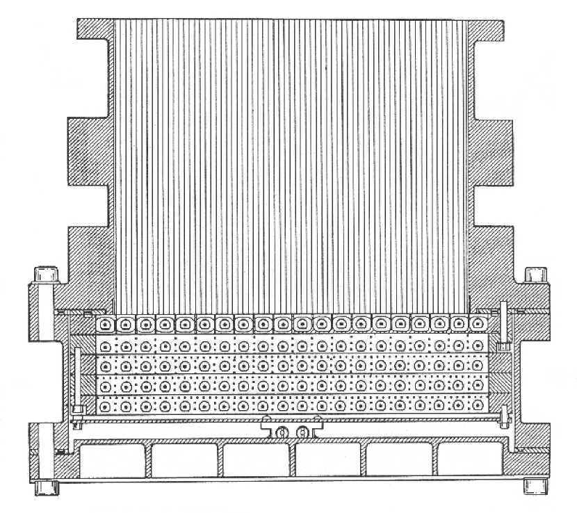
Figure 1: Cross section view of one PCA detector. The field of view is defined by the collimator. Below the collimator, there is a mylar window above and below a propane veto volume. The main xenon-filled detector volume consists of 3 layers of signal anodes and a back layer of veto anondes. Below the veto layer, there are two short anodes on either side of the Am²⁴¹ calibration source. Hatched areas in this figure represent the Aluminum counter body; the Tin and Tantalum shielding is not shown.

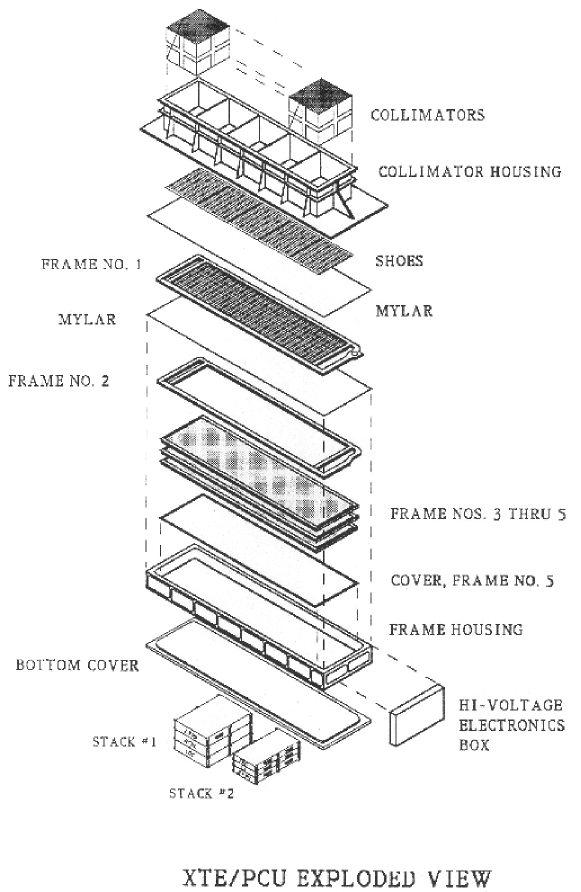
Figure 2: Assembly view of one PCA detector. The field of view is defined by the collimator. The “frames” hold the anodes which define the various detector layers. The propane anodes are in frame 1; the first Xenon signal layer is defined by frame 2; frames 3 through 5 define the second and third Xenon layers and the Xenon veto-layer. The calibration source, not visible in this view, is mounted on the back of the frame 5 cover.

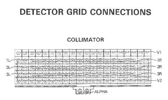
Figure 3: Anode interconnections within a PCU. The chain labelled “V1” is usually referred to as the “Propane” layer; the chain labelled “V2” is usually referred to as the “veto” layer or “$V_{x}$” chain. Activity on either of these chains is treated as a coincidence flag that inhibits further analysis of simultaneous events on the main signal layers.

The PCA consisits of 5 nominally identical Proportional Counter Units (PCU). Each has a net geometric collecting area of $\sim 1600\,{\rm cm}^{2}$. Construction, ground performance, and early inflight performance are described elsewhere (Glasser et al, 1994; Zhang et al., 1993; Jahoda et al, 1996). The proportional counters were designed, built, and tested within the Goddard Space Flight Center (GSFC) Laboratory for High Energy Astrophysics. The essential features are visible in the detector cross section (figure 1) and assembly view (figure 2). The detectors consist of a mechanical collimator with FWHM $\sim 1^{\circ}$, an aluminized mylar window, a propane filled “veto” volume, a second mylar window, and a Xenon filled main counter. The Xenon volume is divided into cells of $\sim 1.3\,{\rm cm}\times\,1.3\,{\rm cm}\times 1\,{\rm m}$ by wire walls. The detector bodies are constructed of Aluminum and surrounded by a graded shield consisting of a layer of Tin followed by a layer of Tantalum. Nominal dimensions are given in table 1. There are three layers of Xenon cells, and each layer is divided in half by connecting alternate cells to either the “right” or “left” amplifier chain. These six signal chains are referred to as 1L, 1R, 2L, 2R, 3L, and 3R. The connections are shown in figure 3. The digit denotes the layer while the letter denotes “right” or “left”. The division of each layer is significant for data screening and background modelling. The response matrices for each half of each layer are identical. Scientific analyses generally combine data from the two halves.

There are 3 additional signal chains. The anodes in the front volume are connected together to form the “Propane” chain; events on this chain are presented to the analog to digital coverter. The outermost anode on each layer and the entire fourth layer are connected together to form a xenon veto ($V_{x}$) chain; signals on this chain are not digitized but are presented to the EDS as a two bit pulse height. Finally, two short anodes on either side of the $Am^{241}$ source provide a flag which is interpretted to mean activity on any of the other anodes is likely to be a calibration event. Of course, there is a chance of 50% or more that the calibration photon will go the wrong way or not be absorbed in the active volume. It is also clear from the background spectra that some calibration events are not flagged.

Every event, whether due to background or a cosmic source, passes 19 bits over a serial interface to the Experiment Data System (EDS) . The information includes 8 bits of pulse height for events occuring on the Xenon signal or propane veto layers, 2 bits of pulse height for events on the $V_{x}$ layer, 8 lower level discriminator bits (for the 6 signal chains, Propane chain, and the calibration flag) and a very large event flag. A “ good event” (i.e. an X-ray) is an event which triggers exactly one discriminator; the pulse height bits can be unambiguously associated with that signal chain. For coincidence events there is an ambiguity about which signal was digitized, and these events are typically ignored. The EDS applies a time-tag and performs event selection and (multiple) data compressions. Of particular interest, two standard compression modes have been run throughout the entire mission. Standard 1 provides light curves with 0.125 sec resolution and calibration spectra with full pulse height information collected every 128 seconds. Standard 2 provides pulse height information for each layer of each detector with 16 second resolution and 29 rates which account for all the “non X-ray” events. Both Standard modes count each event produced by the PCA exactly once. Data used for in-flight calibration of the energy scale comes exclusively from the standard modes. Scientific data in the telemetry stream identifies the detectors with a 0-4 scheme.

2.1 Routine Operations

The RXTE spacecraft allows extremely flexible observations, often making more than 20 discrete and scientifically motivated pointings within a day. The data modes are selectable, allowing the compression which is required for bright objects (due to downlink bandwidth) to be performed in a user selected way. More detail about the standard and user selectable data modes is contained in the RXTE user guide. A brief description of creating response matrices for user selected modes, using the ftool script pcarsp, is given in the Appendix. Throughout this paper we use a typewriter font to refer to FTOOLS programs or scripts and an italic font to refer to the associated parameters.

In addition to pointing direction and data compression mode, there are only two user commandable parameters.

Each detector is equipped with a High Rate Monitor (HRM) which disables the high voltage when the total number of counts on any anode exceeds a preset counting rate for three consecutive 8 second intervals. The default is set to 8000 count sec^-1. This rate is occasionally adjusted upwards (typically to 24,000 count sec^-1) for observations of extremely bright sources such as Sco X-1. It is unlikely that the HRM would ever be tripped if set much above 35,000 count sec^-1 as paralyzable deadtime losses prevent any anode from registering more than about this counting rate.

Each detector is also equiped with a selectable Very Large Event window. Events which saturate the pre-amplifiers cause ringing as the amplified signal is restored to the baseline; often the ringing can cause false events to be pushed through the system. The timing of these events is dependent on the actual pulse height of the saturating event. Each detector has 4 commandable windows, set nominally to $20$, $60$, $150$, and $500\,\mu{\rm s}$. The pre-launch intention was to allow “extra clean data” for very faint sources and “high throughput” data for very bright sources. The size of the VLE window affects the shape of the power spectrum (section 6.1). Early observations of Cyg X-1 with the VLE window set to the smallest value demonstrated a failure associated with this window on one of the analog chains; use of the shortest VLE window has been discontinued. The third window is the default; observations of some bright sources have been conducted with the second window. The calibrated values of these two windows are $70$ and $170\,\mu{\rm s}$.

The High Voltage is commandable in discrete steps, and has been changed by the instrument team 3 times during the mission, resulting in discontinuities in the energy response. In addition, the propane layer in PCU 0 lost pressure in the spring of 2000, in a manner consistent with a micro-meteorite induced pinhole. We use the term epoch to describe the periods between these discontinuous changes in the instrument response. Response changes within an epoch are gradual and can be described by parameterizations with a small time dependence. Definitions of the epochs are given in Table 2. Epoch 3 is divided into 3A and 3B as the time dependence of the background model changed significantly within epoch 3; the boundary is near the moment when orbital decay became important as discussed in section 5.

Three of the PCUs became subject to periodic discharge after launch. The discharge is primarily evident in an increased rate on one signal chain, and in extreme cases by a reduced high voltage. (High rates can reduce the voltage by drawing current from the high voltage supply. There is a large resistor between the supply and the input to the pre-amplifier.) This behaviour began in March 1996 for PCUs 3 and 4 and in March 1999 for PCU 1. To minimize the occurence of discharge several operational steps were taken. First, detectors that break down are now cycled off and on and are not used when the scientific objectives do not require large instantaneous area. Second, the high voltage has been lowered. Finally, the spacecraft roll angle has been changed slightly to increase the solar heating of the PCA and to operate at a slighty warmer temperature. While discharge still occurs, the EDS detects these occurrences by comparing the first moment of the pulse height distributions from the two anode chains associated with each layer. When mismatched moments are detected, the EDS sets a status signal detectable in the satellite Telemetry Status Monitoring (TSM) system which causes the high voltage to be turned off. The EDS calculation is performed every 16 sec; the TSM requires 5 consecutive readings (separated by 8 sec), so periods of discharge are limited to less than one minute; resting the detectors for a few hours allows them to be turned on again. In mid-2004, the duty cycles (not counting the fraction of the orbit when all detectors are off due to passage through the SAA, which amounts to $\sim 20\%$) of PCUs 0-4 were $\sim$ 1.0, 0.2, 1.0, 0.6, and 0.2.

The high voltage was lowered in March 1996 and again in April 1996 as new operating procedures were installed after the first breakdowns of PCU 3 and 4. The high voltage was lowered again in April 1999 after the first breakdown in PCU 1. The times are given in Table 2 along with the high voltage settings (pre-launch measurements) within the Xenon detectors.

There was a brief period in March 1999 when the high voltage fluctuated from the desired setting (level 4) to the epoch 3 setting (level 5) due to an error in the high voltage commanding surrounding the South Atlantic Anomaly. The archived PCA housekeeping data correctly records the instantaneous high voltage state.

3 Response Matrix Overview

The response matrix provides the information about the probability that an incident photon of a particular energy will be observed in a particular instrument channel. The PCA response matrices are generated within the standard FTOOLS environment (Blackburn, 1995) and are designed for use with the XSPEC convolution and spectral model fitting program (Arnaud, 1996). A satisfactory matrix must account for

• The energy to mean channel relationship

• the quantum efficiency as a function of energy

• the spectral redistribution within the detector

We describe below the model as implemented by the program pcarmf as released in FTOOLS v5.3 in November 2003. The ftool pcarmf produces a 256 channel response matrix for a single detector or detector layer. The appendix describes the additional steps needed to produce a response matrix any of the rebinned and compressed modes commonly used by the PCA and found in the RXTE archive.

3.1 Energy to channel model

The energy to channel relationship in proportional counters is non-monotonic in the neighborhood of atomic absorption edges (Jahoda and McCammon, 1988; Bavdaz et al., 1995; Tsunemi et al., 1993). The mean ionization state of an atom which absorbs a photon just above an atomic absorption edge is greater than the mean ionization state if the photon is just below the edge. Because more energy goes into potential energy assoicated with the absorbing atom, the photo-electron (and other electrons ejected from the atom by Auger or shake-off processes) have less kinetic energy and the mean number of electrons produced in the absorbing gas is smaller. Between edges, the energy available for ionizing the gas increases smoothly as does the mean number of electrons created as the final result of the photo-electric absorption (dos Santos et al., 1993, 1994; Borges et al., 2003).

While the voltage pulse in a “proportional counter” is only approximately proportional to the incident photon energy, the pulse is proportional to the number of electrons produced in the absorption region. The observed pulse heights are just the number of electrons produced in the gas multiplied by the electronic gain from both the proportional counter itself and the amplifier chains. The response matrix provides the probabilities that an X-ray of a particular energy ($E_{\gamma}$) will be observed in each of the detector pulse height channels (numbered 0 through 255). When analyzing or plotting the data, it is often convenient to label the channels with energies. Plotting pulse height spectra as a function of energy is facilitated by a single valued channel to apparent energy relationship. We define a second scale, $E_{p}$, proportional to the number of electrons produced and normalized to be approximately equal to energy by taking advantage of the detailed predictions about the number of electrons produced by photo-electric absorption in Xenon (Dias et al., 1993, 1997). A cut through the response matrix gives the probabilities that a photon of energy $E_{\gamma}$ will be observed at apparent energy $E_{p}$. The matrix captures both the non-linearities in the this relationship and the instrumental redistribution. The XSPEC spectral convolution program provides the option of plotting or data selection using the $E_{p}$ or channel scale.

The average number of eV ($w$) required to produce one ionization electron in Xe is shown as a function of photon energy ($E_{\gamma}$) in figure 4. The values of $w(E_{\gamma})$ are near 22 eV and we define

$$E_{p}={22.0\over{w(E_{\gamma})}}E_{\gamma}.$$ (1)

With this definition there are discontinuities of 76.4, 10.9, and 12.6 eV in $E_{p}$ at the Xenon $L_{1}$, $L_{2}$, and $L_{3}$ edges with $E_{\gamma}=4.78,5.10,{\rm and}\,5.45$ keV and a discontinuity of 173 eV at the Xe $K$ edge at 34.5 keV.

We find that the PCA data are better fit with smaller jumps, and introduce a parameter $f$ which lessens the difference between $E_{p}$ and $E_{\gamma}$ and reduces the size of the jumps. For values $0\leq f\leq 1$ we define

$$w_{f}(E_{\gamma})=(w(E_{\gamma})-22.0)f+22.0.$$ (2)

The value of the parameter $f$ is optimized in our fitting procedure. Our best fit value for $f$ is 0.4, resulting in a total jump of 40 eV summed across the three edges.

Our response matrix has an “instantaneous” quadratic relationship between channel and $E_{p}$. Within each high voltage epoch we fit a model where

$$ch(E,T)=A+BE_{p}+C_{o}E_{p}^{2}.$$ (3)

The constant and linear coefficients are time dependent:

$$A=A_{0}+A_{1}\Delta T+A_{2}(\Delta T)^{2}$$ (4)

and

$$B=B_{0}+B_{1}\Delta T+B_{2}(\Delta T)^{2}E_{p}.$$ (5)

$\Delta T$ is the time in days between $T$ and a reference date $T_{0}$. The cause of the time dependence is not known, but may reflect a slow change in purity or pressure of the gas or other changes within the amplifier chain.

3.2 Quantum Efficiency

To model the quantum efficiency, each PCU is treated as a series of parallel slabs of material. No account is made of possible bowing of the front entrance aperture on any scale. All quantum efficiency parameters, specified in pcarmf.par and documented in table 3, are reported with units of gm cm^-2:

We specify for each detector

• Xe_l(m), the amount of Xenon in detector layer $m$; $m$ runs from 1 to 3. 1 represents the top layer and 3 the innermost layer as seen from the collimator (figure 3);

• Xe_pr, the amount of Xenon in the propane layer on 1997 Dec 20;

• $d({\rm Xe}_{pr})/dt$, the rate of change (per day) of Xenon in the propane layer;

• Xe_dl, the thickness of a dead layer of Xenon between adjacent layers;

• $Mylar$, the total thickness of the two Mylar windows;

• $Aluminum$ The total amount of aluminization on the four sides of the two windows;

• $Propane$ The amount of propane in the first gas volume

The dead layer, as modelled here, assumes that there is a small region where events will be self vetoed as part of the electron cloud is collected in one anode volume and part in the adjacent volume. In detail, such a region probably has a soft edge, though our data cannot distinguish this. Additionally, the model requires that PCU 0, despite the loss of pressure in the propane layer, requires residual Xenon in the propane layer in epoch 5. The best parameterization requires half as much Xenon as before the loss of pressure. This model is unsatisfactory, and the fits are less good for PCU 0 in epoch 5. There could be many causes, including bowing of the internal window which now supports a 1 atm pressure differential.

The Xenon absorption cross sections are from McMaster et al. (1969). All other absorption cross sections are derived from Henke et al. (1993).

Figure 5 shows the modelled quantum efficiency for PCU 2, layers 1, 2, 3 on January 13, 2002. The peak quantum efficiency has decreased by $\sim 1\%$ per year over the lifetime of the mission due to the diffusion of Xenon into the front veto volume.

3.3 Redistribution matrix

Our model accounts for the intrinsic resolution of the proportional counter, K and L escape peaks, losses due to finite electron track length (which causes events to be self-vetoed), and losses due to partial charge collection (which causes events to show up in a low energy tail). These contributions are described in more detail below.

Proportional counter resolution is typically limited at high energies by fano factor statistics. At low energies there may be a significant component related to detector non-uniformities and readout electronics (Fraser, 1989). The resolution ($\Delta E/E$, where $\Delta E$ is the FWHM) is $\sim 0.17$ at 6 keV and $\sim 0.08$ at 22 keV, measured with ground calibration sources. We model the resolution (FWHM) in channel space as

$${\Delta ch}=(\sqrt{aE+b})B$$ (6)

where $B$ is the slope term from equation 3.

The Xenon L-escape peak is not prominent. The 4.1 keV escape photon has a mean free path of 0.5 cm in 1 atm of Xenon. Escape is only possible from the first layer. For the inner layers (and the front layer) there is a chance that the escape photon will be re-absorbed in an adjacent layer. The resulting coincident signals will affect the overall efficiency as the EDS will not recognize this as a good event. The model allows an efficiency correction for energies above the Xenon L-edges and below the K edge, though our parameterization sets this self vetoed fraction to 0. The overall normalization is adjusted by the values of geometric area which parameterize the tool xpcaarf.

Above the K-edge, only the K-escape peaks are modelled, and these are more prominent than the main photo-peak. Detailed prediction of the amplitudes would require a complex integration over the detector geometry, and might be slightly different for the three detector layers. We assume that the escape fraction is the same for each layer. Initial estimates of the escape fractions come from laboratory data obtained at the Brookhaven National Laboratory National Synchrotron Light Source where small areas of one of the detector were illuminated by monochromatic beams. Our model allows a correction for self vetoing events when the escape photon is absorbed in a different anode volume. Our estimate is that 0.09 of the events above the K-edge are vetoed by the reabsorption of an escape photon in a different signal volume. The ratio of events in the photo-peak, the $K_{\alpha}$ escape peak, and the $K_{\beta}$ escape peak is 0.29 / 0.55 / 0.16. The redistribution function for a 50 keV input is illustrated in figure 6.

Events can be lost if the photo-electron travels into a second anode volume. Youngen et al. (1994) demonstrated the importance of this effect for the HEAO-1 A2 High Energy Detector (Rothschild et al., 1979) which has a similar internal geometry to the PCA. The Youngen model is a Monte Carlo, making it difficult to use the results directly. We model the unvetoed fraction as

$$f_{unveto}=1.0-A_{o}g(layer)({E_{electron}\over E_{point}})^{\delta}$$ (7)

where $E_{electron}$ is the energy of the initial photo-electron, $A_{o}$ is an amplitude, $E_{point}$ is an empirical parameter that is approximately the energy where this effect becomes important, and the factor $g(layer)$ (= 1, 1.33, 1.33 for the first, second, and third layers) accounts for the fact that the inner detection cells have more edges which the electron might cross. Because the exponent $\delta$ is large ($\sim 3$), the fraction lost is near constant below $E_{point}$ and rises quickly above this energy.

We also model partial charge collection. For X-rays which are absorbed near the edge of the active region, there is a competition between diffusion and drift towards the high field region where charge multiplication occurs. The effect has been modelled at low energies (Inoue et al., 1978) and parameterized in terms of the ratio $\kappa={D\over{w\lambda}}$ where $D$ is the diffusion coefficient, $w$ is the drift velocity, and $\lambda$ is the mean absorption depth. For an initial cloud of $N_{o}$ electrons, the number which reach the amplification region is

$$f(N)dN=\kappa(1-{N\over N_{o}})^{\kappa-1}dN.$$ (8)

Jahoda and McCammon (1988) used this equation directly for an Argon based counter while Inoue et al. (1978) found it necessary to introduce an ad-hoc factor of $\sim 3$ for a Xenon based counter. We have chosen to treat the ratio of $D$ and $w$ as a free parameter which we fit. Equation 8 was derived for energies where the photons are absorbed near the entrance window. However, this model predicts very small losses for energies where this condition is not satisfied, so we apply this model at all energies.

Figure 6 shows the redistribution function for lines with energies at 5, 9, and 50 keV to illustrate the magnitude of the incomplete charge collection, L-escape, and K-escape peaks. The normalization of the lines is arbitrary and selected for illustrative purposes.

3.4 Detailed construction of the matrix

This section describes the operation of the PCA response generator pcarmf; default values of the parameters and their mnemonics are listed in table 3 and described below.

The matrix is constructed to have 296 energy bins in $E_{\gamma}$, spaced logarithmically from 1.5 to 80.0 keV. Extra bin boundaries are inserted at the three Xenon L edges and the Xenon K edge, so there are a total of 300 energy bins. The edge energies are read as the parameters xeL3edge, xeL2edge, xeL1edge and xeKedge. The matrix maps monochromatic input from the mean energy of each bin to 256 detector channels, indexed from 0 to 255 to match the channel-ids reported by the PCA to the EDS.

The response matrix generator works on one detector and one layer at a time. The detector is specified by pcuid with allowed values ranging from 0 to 4. The layer is specified by lld with allowed values of 3, 12, 48, 63, and 64 for the first, second, third, summed Xenon, and propane layers respectively. The date is specified by cdate, in yyyy-mm-dd format.

A matrix corresponding to the selected detector, layer, and date is generated with the following steps. For each energy in the matrix we

• Determine the overall quantum efficiency.

• Calculate $E_{p}$ (equations 1 and 2); the parameter $f$ is specified by w_xe_fact.

• Calculate the mean channel ($ch_{mean}$). The coefficients in equation 3 are stored in pca_e2c_e05v03.fits found in the $LHEA_DATA directory which is part of the FTOOLS v6.0 package. The latest version of this file is also available from the HEASARC calibration data base CALDB.

• Determine whether the photon energy is below the Xenon L3 edge (parameter xeL3edge) where no escape peak is possible, between the L3 and K edge (parameter xeKedge) where an L-escape photon is possible, or above the K edge where both the Xe K_α and K_β escape photons are possible.

• For energies where escape peaks are possible, calculate the mean channel of the escape peak. Monte Carlo and experimental results (Dias et al., 1996) indicate that the mean channel associated with an escape peak is not in the same location as the photo-peak for an X-ray with energy equal to $E_{\gamma}-E_{esc}$. The offsets can be as large as 70 eV and are quantified in terms of a number of electrons; the offsets are parameterized as delta_el_L, delta_el_Ka and delta_el_Kb for the L, K_α, and K_β escape peaks respectively. The default values, taken from Dias et al. (1996) are 3.9, -2.26, and 3.84 electrons respectively.

• For energies where K escape peaks are possible, the fraction of events in the escape peak are given by EscFracKa and EscFracKb for the K_α and K_β peaks respectively. The fractions are modelled to be the same for each layer in the detector. When K escape peaks are possible, the L escape fraction is modelled to be 0.

• For energies where the L escape peak is possible, the fraction of events in the escape peak is given by EscFracLM where M is 1, 2, or 3 corresponding to the layer that the photon is absorbed in. The default parameterization is no L escape peak for photons absorbed in the second or third layer, and $1\%$ for photons absorbed in the first layer.

• For the main photo-peak, evaluate the resolution. The coefficients $a$ and $b$ in equation 6 are given by resp1_N and resp2_N where $N$ identifies the PCU. These coefficients have not been separately fit by PCU. The resolution is assumed to be constant in in keV; the coefficient $B$ converts the resolution in keV to the (time dependent) value in channels.

• Correct the quantum efficiency for the effects of electron tracking (equation 7) where the coefficients $A_{o}$, $E_{point}$, and $\delta$ are given by track_coeff, epoint and track_exp.

• Distribute the corrected quantum efficiency, further corrected for the escape fractions, in a gaussian centered at $ch_{mean}$ and with $\sigma=\Delta ch/2.35$

• Treat the escape peaks similarly. The resolution and electron tracking are calculated for $E_{\gamma}-E_{esc}$, and the resulting peaks are added to the 256 channel spectrum.

• Correct the entire 256 channel spectrum for partial charge collection (equation 8). As noted above, this is certainly unphysical for large energies, but the effect is small here, and the model is plausibly correct at the energies where the effect is important.

4 Calibrating the parameters

4.1 Calibration Sources and Targets

Data suitable for parameterizing the energy scale, and monitoring variations, comes from three regularly observed sources: the internal calibration source provides continuous calibration lines at 6 energies from 13 to 60 keV; approximately annual observations of Cas A provide a strong and well measured Iron line at 6.59 keV; and regular monitoring observations of the Crab nebula provide an opportunity to measure the location of the Xenon L-edges near 5 keV. Almost all of the ground calibration data was obtained with High Voltage settings that correspond to Epoch 1. In addition no ground data was obtained which illuminated an entire detector. Ground calibration thus verified basic operation of each detector and the general features of the response. The detailed response is parameterized with flight measurements, which also allows a correction for a small time dependence.

4.1.1 Internal Calibration Source

Each PCU contains a small Am²⁴¹ source which provides a continuous source of tagged calibration lines with energies between 13 and 60 keV (Zhang et al., 1993). The energies and notes about each line are listed in table 4. Calibration spectra are telemetered with the full 256 channel resolution of the PCA, so we perform fits directly in channel space. A sum of 6 gaussians with a small constant and linear term provides an excellent fit. An example is shown in figure 7. The 60 keV line is imperfectly modelled by a Gaussian as the Compton cross section is beginning to become significant with respect to the photo-electric cross section. We have ignored this effect.

We collected calibration data from dedicated sky background pointings within each calender month of the mission (for the period before November 1996 when dedicated background observations began, we have used observations of faint sources). During months when the high voltage changed, we collected 2 distinct spectra. This procedure provides data which is systematics (i.e. not statistics) limited. For instance, the line near 26 keV is consistently broader than the others as it is a blend of a nuclear line from the Am²⁴¹ source and the K-$\alpha$ escape peak from the 60 keV line.

4.1.2 Cassiopeia A

The supernova remnant Cassiopeia A has a bright, strong, Iron line easily visible in the PCA count spectra. Cas-A has been observed approximately annually as a calibration source, and we have fit a model with a power law continuum and a gaussian line to the data between 4 and 9 keV (figure 8). Over this band pass, this simple model provides an acceptable fit to the data; over a broader band the models become quite complex (Allen et al., 1997). The fit energy centroid can be unambiguously converted to a mean channel. We assume that the actual average energy of the Fe line complex is 6.59 keV, consistent with Ginga (Hatsukade and Tsunemi, 1992) and ASCA (Holt et al., 1994) results. The mean channel can be accurately determined without considering the line complex at 8.1 keV observed by Pravdo and Smith (1979) and Bleeker et al. (2001).

While there are relatively few pointings at Cas-A, and this line thus has limited weight in the channel to energy fits, it does provide a valuable check on the accuracy of the energy scale in the Fe line vicinity. Results are presented in section 4.5. While calibration near the Iron line is unavailable for the second and third Xenon layers, there is also little significant signal from cosmic sources here.

4.1.3 Xenon L-edge

Each detector has a front layer filled with propane; a small amount of Xenon is also present, due to diffusion either through the window or the o-ring seal that separates the two volumes. Although the presence of Xenon in this layer does reduce the efficiency in the active volume, it also provides a calibration opportunity. The regular monitoring of the Crab nebula plus pulsar allows us to measure and monitor the energy calibration near the Xenon L-edge at 4.78 keV.

The response matrices with default parameters account for the Xenon in the propane layer, however we can construct a matrix which artificially sets the amount of Xenon to zero. The Crab continuum spectrum, analyzed with this incorrect matrix, requires an absorption edge to mimic the unaccounted for Xenon. Fits to this edge can be interpretted in terms of the energy scale.

We perform fits in energy space, and convert the fit energy back to channels. The resulting set of date/channel pairs for 4.78 keV are fed back into the procedure that determines the energy to channel relationship.

The Xenon L-“edge” has structure on a scale that is fine with respect to the energy resolution of the PCA. There are 3 edges with energies at 4.78, 5.10, and 5.45 keV. With proportional counter resolution these cannot be fit simultaneously. We use a model with a power-law, 3 edges, and “interstellar absorption” with variable elemental abundances; the absorption and edges mimic the absorption due to the Xenon in the propane layer. The energies of the second and third edges are fixed at 1.07 and 1.18 times the energy of the first edge, and the optical depth is fixed at 0.44 and 0.18 times the optical depth of the first edge (Henke et al., 1993). The absorption uses the XSPEC varabs model, itself based on the cross-sections tabulated by Balucinska-Church and McCammon (1992). We keep the relative abundances of H, He, C, N, O, and Al fixed with respect to each other. The abundance of Fe is allowed to vary. The abundances of all other elements are fixed at zero. This description is not intended to be physical, but rather to produce a fit with small residuals; examples are shown for PCU 2, layers 1 and 2, in figures 9 and 10.

The edges are quite precisely fit with typical $3\sigma$ errors less than $\pm 0.07$ keV for the first layer. We include over 100 observations in our determination of the energy to channel law, and the average is extremely well determined. Systematics associated with the model are thus quite important, and it remains possible that a different parameterization of the edge could provide a matrix with smaller residuals in the vicinity of the L-edge (see section 4.5.2).

4.2 Energy to channel relationship

We fit the energy to channel relationship separately for each detector, layer, and epoch using a $\chi^{2}$ minimization. Figure 11 shows the data that goes into this fit for PCU 2. The upper panel shows the centroids fit to the 6 peaks in the calibration spectra on a monthly basis; the lower panel shows the channels fit to the Xenon L-edge from Crab monitoring observations and the Iron line fit to approximately annual observations of Cas A. The gaps in the Xenon L edge data correspond to the annual period when the Crab is too close to the sun to be observed.

The precision of the input data is highest at energies well above the PCA peak sensitivity. The errors on the calibration line channels, as a fraction of the channel, range from $10^{-3}$ for the lines at 13 and 21 keV to less than $5\times 10^{-4}$ for the lines at 17, 30 and 60 keV. The fractional errors on the L-edge channel and Cas-A line are $\sim 5\times 10^{-3}$. The errors on the Cas-A line energy include a statistical component and are correlated with exposure time.

The mean photon energy observed by the PCA is always below 10 keV; to apply the maximum weight to the points nearest this mean, we reduce the error associated with the L-edge points by a factor of 10. To apply approximately equal weight to each of the Cas-A points and remove the exposure dependence, we set all errors to 0.1 channel (about the mean). We are not using the chi-square minimization to estimate errors on the channel to energy parameters (equation 3) and we validate the results by examining the fits to the Crab nebula (section 4.5.2). This ad-hoc procedure for adjusting the errors is justified not by statistical rigor, but by reasonable results. Our fits are consistently poor for the line near 26 keV; we attribute this to poor knowledge of the mean energy of this blended line, and exclude it from our fits.

We produce energy to channel parameters for a range of values of the parameter $f$ (eq. 2); selection of the best value of $f$ comes after the process of adjusting the parameters associated with quantum efficiency and redistribution.

4.3 Quantum efficiency and redistribution

The response matrix contains many correlated parameters; we have used our frequent observations of the Crab nebula to make numerous estimates of the best values of the parameters, and then made a response matrix using averages over time, or over time and PCU.

For each observation of the Crab, we have collected the data and estimated the background separately for each layer of each detector. We use the channel to energy law to select data from each layer with $E_{min}(layer)\leq E_{p}\leq E_{max}(layer)$. For the first layer we use $E_{min}$ = 3 keV and $E_{max}$ = 50 keV; for the second and third layers we accept data from 8 to 50 keV.

These data are fit, via a chi-square minimization technique, to a model which parameterizes the response matrix and the Crab input spectrum. As parameters are highly correlated (i.e. the amount of Xenon in the first layer and the power law index for the Crab) we have adopted a procedure that minimizes a few parameters at a time, and revisits earlier steps as needed. The Crab photon index is fixed at $-2.1$ and interstellar column density is fixed at $3\times 10^{21}$ H atoms ${\rm cm}^{-2}$ using the approximation to absorption given Zombeck (1990) (page 200).

Figure 12 shows the resulting fit values for the Xenon thicknesses of the first and second signal layers, the propane volume, and the dead layer for PCU 2. We require the Xenon thickness of the third layer to be equal to the second layer. The time scale is in days relative to 20 Dec 1997. Note that on this plot there is no discernable break in March 1999 (near day 500) when the high voltage was changed.

This procedure was repeated for several values of the parameter $f$. We selected the best value of $f$ by comparing the values of $\chi^{2}_{red}$ for power law fits to the Crab data in all three layers. By design all of these fits returned $\Gamma\approx 2.1$. Using $\chi^{2}_{red}$ as a discriminating statistic, there is smooth variation with $f$, as shown in fig 13. For almost all observations of the Crab with $0.35\leq f_{min}\leq 0.45$, so we adopted $f=0.40$ as the best fit value. The calibration of the Ginga Large Area Counters reports a total jump of 70 eV (equivalent to $f\approx 0.7$) summed across the three Xenon edges (Turner et al., 1989). The discrepancy in $f$, which represents the properties of Xenon rather than detector details, indicates that systematics remain in the Ginga and/or PCA models.

Table 3 gives the best fit values for the parameters. The parameters are more similar from detector to detector than for previous calibrations which were performed with a more ad-hoc approach.

4.4 Effective Area

We adjusted the areas in xpcaarf so that we match the canonical Crab flux (Zombeck, 1990). Individual spectra from the Crab were corrected for both instrumental and source induced deadtime (typically $\sim 6\%$; see fig 30.) Following this, the area parameters in xpcaarf were adjusted so that the best fit flux matches the literature values. The net geometric areas were subjected to an upwards correction of $\sim 12\%$. The absolute error in flux scale is believed to be smaller than this; in situations where absolute measurements are attempted, it is thus important to correct for deadtime. Our correction removes a substantial fraction of the discrepancy noted by, e.g., Kuulkers et al. (2003) and references therein, which was performed with a previous version of the response generator, which also systematically reported higher values of the photon index for the Crab.

Our procedure is to fit an absorbed power-law to the many observations of the Crab nebula. We use data from the first layer, and adjust the peak open area of the detector so that the average 2-10 keV flux is $2.4\times 10^{-8}\,{\rm erg}\,{\rm sec}^{-1}\,{\rm cm}^{-2}\,$ (Zombeck, 1990). The derived geometric areas, which are inputs to xpcaarf, are documented in table 3. For PCU 0 we use data only from epoch 3 and 4 as the epoch 5 calibration remains poor (see the step function in the best fit index in fig 15).

The PCA flux scale remains higher than for other instruments as the adopted flux scale ignores interstellar absorption and because the the Zombeck (1990) parameterization of the Crab nebula plus pulsar provides the highest inferred 2-10 keV flux amongst measurements of the absolute flux. More details about the flux scale are provided on the PCA web page (footnote 3).

4.5 Checks on the Quality of the Redistribution Matrix

4.5.1 Energy scale

We re-fit the Cas-A line with our best fit matrix and plot the results in fig 14. The fits return a narrow line. The centroid position is fit only to $\sim 0.15$ keV due to a combination of the intrinsic resolution of the detector and the steepness of the underlying continuum ($\Gamma\approx 3$). These errors are representative of the accuracy that can be expected from fits to strong lines.

We have examined the stability of the energy scale on short time scales by collecting the Am²⁴¹ calibration spectra on 1000 second intervals, taking data from all periods when the detectors were on. Such spectra allow fits for the amplitude and centroid of the six lines although it is necessary to fix the width of the peaks at values fit to spectra collected over one day. We find no evidence for gain variation on any timescale longer than 1000 seconds, and no effect on gain with respect to source counting rate. (up to 2 Crab in the days we examined).

4.5.2 Spectrum of the Crab Nebula

The Crab offers three checks on the quality of the response matrix. First, it allows us to establish consistency with previous results since the integrated emission is believed to be time stationary. Second, it allows us to establish whether our matrix properly accounts for the time dependencies in the detectors, and provides the same results over the nearly nine years (and counting) lifetime of the mission. Third, we can examine the residuals to the fits and thus estimate how large residuals in fits to other sources must be before simple continuum models are deemed inadequate.

The first two points are addressed in figures 15 through 19 which present the best fit power-law index for about one-quarter of the Crab monitoring observations using the matrix generator in the FTOOLS v5.3 release (crosses), as well as the previous calibration (open squares). The substantive differences between the two releases are

• More Crab and background data is included, thus better specifying the slow drifts in the channel to energy relationship;

• the parameters for each detector are minimized with the constraint that the power law index of the Crab be -2.1; this improves the detector to detector agreement with a modest increase in chi-squared.

• an error in the calculation of the instrument resolution (equation 6) was repaired.

For all fits the interstellar absoprtion was fixed at a column density of $3\times 10^{21}$ H atoms ${\rm cm}^{-2}$ using the XSPEC model wabs. The lower panel in each figure shows the reduced $\chi^{2}$ associated with the FTOOLS v5.3 and v5.2. By construction, the best fit power-law index is now more consistent from PCU to PCU (particularly at late times where the previous calibration provided an estimate based on extrapolation). These figures show fits to layer 1 only, which provides the large majority of the detected photons and the largest bandwidth. That the reduced $\chi^{2}$ is typically greater than 1 indicates that unmodelled systematics remain.

The data and model, along with the ratio of data to model, fit to a representative Crab monitoring observation are demonstrated in figures 20 and 23. The data are from 1999-02-24 and the best fit power law indices are 2.088, 2.098, 2.105, 2.088, and 2.096. The deviations from the power law are quite similar from one detector to the next. Figure 21 shows an enlargement of the 3-20 keV region; below 10 keV the deviations are less than $1\%$. Between 10 and 20 keV the data begins to exceed the model slightly, though only by $\sim 2\%$. There is a clear underprediction just below the Xenon K edge; although this is quite obvious in the ratio presentation, the number of counts per channel (the convolution of the intrinsic spectrum with the detector quantum efficiency, both of which decline rapidly with energy) is nearly three orders of magnitude below the peak. Figure 22 shows the contributions to $\chi^{2}$, which are dominated by deviations at the lowest energies and near the Xenon L edge, where the counting rates are high.

Figure 23 shows fits to data from all three layers. The data are from 2003-02-26, PCU 2; the power law indices are constrained to be the same (best fit 2.123) The normalizations are allowed to float; the variation (max to min) is less than 3%. Requiring the normalizations to be the same does not change the best fit index.

5 Background model Overview

The RXTE PCA is a non-imaging instrument; for both spectroscopy and light curve analysis the background must be subtracted based on an a priori model. “Background” is defined broadly to include anything that contributes non-source counts to the PCA instrument in orbit, including but not limited to:

• local particle environment;

• induced radioactivity of the spacecraft; and

• the cosmic X-ray background.

In general, these components vary as a function of time, and must be parameterized. The parameterized model is adjusted to fit a set of dedicated observations by the PCA of blank sky regions. Once a good fit is achieved, the same parameterization can be applied to other observations. The cosmic X-ray background, which in the PCA band is due to the integrated effect of unresolved sources in the field of view, has spatial fluctuations of approximately $7\%(1\sigma)$ (Revnivtsev et al., 2003) in the 2-10 keV band. These fluctuations are not (and cannot) be predicted by the background model; the magnitude of these fluctuations sets the limit below which fluxes cannot be determined by the PCA. This confusion limit is at $4\times 10^{-12}\,{\rm erg}\,{\rm sec}^{-1}\,{\rm cm}^{-2}\,$.

Figure 24 shows the spectra of the “good” count rate during observations of blank sky; this is the total (i.e. instrument plus sky) background. Spectra are shown separately for the first, second, and third layers. The peaks near channels 26 and 30 keV are due to unflagged events from the Am²⁴¹ calibration source. The fractional contribution of sky background to each layer is shown in the lower panel. The sky background is approximately 1 mCrab per beam. The lower light curve in figure 25 shows the total background rate over a two day period of nearly uninterrupted observations of blank sky. Variations by more than a factor of 2 in a day, and by up to a factor of 1.5 in an orbit are clearly visible.

The background models for the PCA have components quite similar to those for the Ginga Large Area Counters (Hayashida et al., 1989). The details of the background spectra and the amplitude of the variability are different, as expected, due to differences in the orbit (RXTE has a lower inclination and smaller eccentricity than Ginga) and details of the detector construction. We use data collected over a period of years from repeated observations of several blank sky positions to measure and model the background and its variation.

The most successful background model to date for faint sources is the “L7/240” model. Here, “L7” is the name of a housekeeping rate which is well correlated with most of the variation in the PCA background rate. The L7 rate is the sum of all pairwise and adjacent coincidence rates in each PCU. The “240” component refers to a radiactive decay timescale of approximately 240 minutes. This timescale may describe the combined effect of several radioactive elements. The L7/240 model is not appropriate for bright sources because the L7 rate can be modified by the source itself.

The “Very Large Event” housekeeping rate is also correlated with the observed background rate, although with more unmodelled residuals than the L7 rate. Both the L7 and VLE rates are shown in figure 25. Gaps in the blank sky and L7 rates exist due to observations of other sources while the VLE rate is shown throughout, and is virtually unaffected by even bright X-ray sources. Since the VLE rate is largely unaffected by the source rate, it can be used to parameterize a model suitable for “bright” sources. Operationally, bright is defined to be 40 source counts sec^-1 PCU^-1 or about 15 mCrab.

The background model is determined by fitting high latitude blank sky observations which are regularly obtained in 6 directions. The output of the background model is an estimate of the combined spectrum of instrument background and the Cosmic X-ray Background observed at high latitudes. The model makes no attempt to predict the diffuse emission associated with the galaxy (Valinia and Marshall, 1998).

When background observations were begun in November 1996, one day was devoted to this project every three or four weeks. Eventually this was supplemented by short, twice daily observations to better sample the variations that are correlated with the apogee precession of $\sim 30$ days. Because the orbit apogee and perigee differ by about 20 km and because the particle flux within the South Atlantic Anomaly varies with altitude, the average daily particle fluence, and the radioactive decay component of the background, show a long term variation with this period as well.

The blank sky observations were originally divided among 5 distinct pointing directions. Daily observations of a sixth point were added in order to test the success of the background modelling for the lengthy NGC 3516 monitoring campaign (Edelson and Nandra, 1999). The pointings are summarized in table 5.

The current background models have explicitly linear dependences on L7 (or VLE), the radioactive decay term, and mission elapsed time.

In the construction of these models, we

• accounted for the variance in L7 (or VLE) itself;

• derived coefficients for each Standard2 pulse height channel independently;

• used a modified chi-square approach for low-statistics Poissonian data (Mighell, 1999)

• included data from immediately after the SAA (i.e. included more data than in earlier efforts)

• selected data with a horizon angle of at least 10 deg and with the rates VPX1L and VPX1R (contained within the Standard2 data) less than 100 sec^-1

The fitted background model for each channel,i, is:

$$BKG_{i}=A_{i}+B_{i}*L7+C_{i}*DOSE+D_{i}*(t-t0)$$ (9)

where $A_{i}$, $B_{i}$, $C_{i}$ and $D_{i}$ are the fit coefficients, L7 is the L7 rate in a PCU, DOSE is the SAA particle dosage summed over individual passages through the SAA and decayed by a 240 minute folding timescale, and t is the epoch time. The SAA particle dosage is measured by the particle monitor on the High Energy X-ray Timing Experiment (Rothschild et al., 1998) also aboard the RXTE; each passage is defined as the period when the HEXTE high voltage is reduced. Equation 9 is linear in all its terms, and allows for a secular drift over time. The predicted model is also stretched (or compressed) to account for the time dependence in the energy to channel relationship (equations 3 and 5). The correction contains only a linear term derived from the peak shifts in the $Am^{241}$ spectra (and is thus slightly inconsistent with the treatment in the response matrix generator).

The secular drift in time has been $\sim 0.07$ ct s^-1 PCU^-1 yr^-1 from epoch 3B through the present, and is well correlated with satellite altitude. This term became significant when the RXTE orbit began to decay. We parameterize the time dependent term as a linear trend within each epoch; there is a discontinuity in the slope at epoch boundaries, with the significant discontinuity at the beginning of epoch 3B corellated with the time when the satellite orbit began to decay noticeably (fig 26). The orbit decay is understood to be due to increased drag as the earth’s atmosphere expanded in response to increased solar activity associated with the solar cycle. The satellite altitude has changed from 580 km at the beginning of epoch 3B to $\sim 500$ km in fall 2003. The secular drift term is not currently included in the VLE models. An effort is underway (in late 2005) to divide epoch 5 into three distinct sub-epochs for the purpose of background estimation. This will allow a more precise estimate of the secular term which is apparently correlated with the change in altitude, and will result in background models constructed from more nearly contemporaneous data, minimizing effects due to the slowly drifting energy to channel relationship. These models will be available from the RXTE web site.

VLE models require a second activation time scale; the second DOSE term is decayed by a 24 minute time scale. Attempts to fit the time scales are poorly constrained, probably due to the fact that both timescales are a mixture of several radioactive half-lives; additionally, for the shorter timescale the DOSE term, which sums the fluence of particles on orbital timescales, may not contain enough time resolution. The quality of the resulting background spectra has been high enough that a more careful parameterization has not been needed, and we have not succeeded in identifying particular radioactive decays that are responsible. All of the identified variations were also observed by the Large Area Counters on Ginga, although with different amplitudes related to the details of the orbit and detector construction (Turner et al., 1989; Hayashida et al., 1989)

Figures 27 and 28 show the coefficients $B_{i}$ and $C_{i}$ for PCU 2, layer 1, during epoch 5 and show that the background varies in both amplitude and spectrum.

The fitting was applied to multiple, dedicated, PCA background pointings. Each of the points on the sky has a slightly different sky background. Our approach is to assign a different set of coefficients $A_{i}$ for each background pointing. The production background model is determined by taking the weighted average of $A_{i}$’s for different pointings. Thus, the background model represents an “average” patch of high latitude sky.

Remaining count-rate variations after background subtraction are a measure of systematic error. We calculated the variance of blank sky rate minus predicted background rate and compared that variance to that expected from counting statistics alone. The difference between these two variances includes unmodelled effects. Figure 29 gives the systematic error per channel while Table 6 gives some band averaged values for individual layers of each detector. In each case we report the square root of the excess variance as a fraction of the total rate; the table also gives an absolute value in counts per sec. The upper line in figure 29 includes a contribution due to the limited precision with which the L7 rate is measured in any single 16 sec bin. For observations of faint sources with the PCA, the systematic errors in the count rates reported in table 6 become larger than the Poisson uncertainties in the count rates for observations longer than a few hundred seconds.

6 Timing Calibration

Every event detected within the PCA, whether a cosmic X-ray or an instrument background event, produces 19 bits which are passed to the EDS which adds the time stamp and performs event selection and rebinning.

Each signal chain has its own analog electronics chain consisting of Charge Sensitive Amplifier, Shaping Amplifier, Discriminator, and Peak Finder. The deadtime associated with the analog chains is paralyzable. The six Xenon signal chains and the Propane signal chain share a single Analog to Digital Converter which produces a 256 bit pulse height; the Xenon veto chain is separately analyzed and produces a 2 bit pulse height. The Analog to Digital Conversion is non-paralyzable. “Good” events produce charge on a single chain; the resulting pulse height can be unambiguously identified with that chain. For events which produce more than one analog signal, the pulse height cannot be unambiguously assigned to a particular chain; such events are generally not included in the telemetry except to be counted in the rates present in the Standard data modes.

6.1 Deadtime

A detailed description of the effects of deadtime on a particular observation depends on both the source brightness and spectrum. The spectrum affects the ratio of events observed in the first layer and other layers, and therefore changes the details of the interaction of a paralyzable deadtime process (associated with each analog chain) and a non paralyzable process (the analog to digital conversion). Fortunately, a complete description is not required for the most needed corrections. We present useful approximations for a common statistical representation of the data (power spectra) and for the construction of light curves.

6.1.1 Power Spectra

Even at relatively low count rates, the probability that events are missed has a significant effect on the shape of the power spectrum (Zhang et al, 1995).

Periods of deadtime can are generated by X-rays or charged particles which interact within the detector. Both the desired astrophysical signal and the instrument background contribute to deadtime.

An X-ray event causes the detector to be dead in two ways. First, it disables its own analog electronic chain, i.e., the Charge Sensitive Amplifier (CSA), Shaping Amplifier (SA), and the associated discriminators for a period of time which depends on the amount of energy it has deposited in the detector; this is a paralyzable dead time. Each detector has 7 analog electronics chains (6 Xenon half-layers and the propane layer) which share an Analog to Digital Converter (ADC). Second, this event causes the entire analog chain to be busy for $10.0\mu{\rm s}$; this is a non-paralyzable dead time which consists of $6.5\mu{\rm s}$ of analog to digital conversion time plus fixed delays to allow the analog signal to settle (prior to the conversion) and for the data to be latched for transfer to the EDS and reset (after the conversion). For events with energy less than $\approx 20$ keV, the analog chain is again live before the end of the ADC conversion. The minimum time between sequential events on the same or different chains is $10\mu{\rm s}$, and to a good approximation, all events can be considered to have this deadtime.

Some events trigger two or more of the analog electronic chains. Most such events are due to a charged particle which leaves a track through the detector. However, a single X-ray can trigger two signal chains, either by creating a fluorescence photon which is reabsorbed elsewhere in the detector, or an energetic photo-electron which travels into an adjacent cell. At high fluxes, it is also possible that two X-rays from the source will be detected simultaneously by different signal chains (van der Klis et al., 1996). In all of these cases, both signal chains are paralyzably dead and one of the signals is presented to the ADC. No information is available to the EDS about which signal was digitized. The ADC deadtime is as above, and $10\mu{\rm s}$ remains a good approximation to the deadtime; for large equivalent energies, one (or more) analog chains may remain dead after the detector as a whole can process another event, just as in the case of an event which triggers a single chain.

An event which triggers the Alpha chain and one additional anode is marked as a calibration event, and produces the same deadtime as any other event of similar energy. An event which triggers only the Alpha chain diables event processing for $6\mu s$ (any event which occurs during this interval will be interpretted as a calibration event.) Events which occur on the $V_{x}$ chain also disable the detector for $6\mu s$ as any event which occurs during this period will be marked in coincidence with the $V_{x}$ event. For events which include the $V_{x}$ chain and a single additional chain, the digitzed pulse height corresponds to the non $V_{x}$ chain. Strictly speaking, events which trigger only $V_{x}$ OR Alpha should not be included in the total deadtime calculation since it is known that no other event was presented to the detector electronics in this interval. This effect is described at greater length in section 6.1.2.

Very Large Events (VLE) are operationally defined as events which exceed the dynamic range of the experiment and which saturate the amplifier. The equivalent energy depends on the high voltage setting, and was $\sim 75$ keV in Epoch 1 and $\sim 120$ keV in Epoch 5. The default VLE window is $170\mu{\rm s}$ (Zhang et al., 1996). See also section 2.1.

The Poisson random noise level is suppressed by the correlation between events caused by the deadtime. To a good approximation, the Poisson noise level with deadtime correction can be computed as follows:

$$P_{d}(f)=P_{1}-P_{2}cos({{\pi f}\over f_{Nyq}})$$ (10)

$P_{1}$ and $P_{2}$ depend in principle on the details of the electronics. For count rates less than $10^{4}$ ct s^-1 PCU^-1 (or $\sim 4$ Crab) the dependence is small and both coefficients can be estimated as if the deadtime is purely paralyzable with

$$P_{1}=2[1-2r_{0}t_{d}(1-{t_{d}\over{2t_{b}}})]{\rm and}$$ (11)

$$P_{2}=2r_{0}t_{d}{{N-1}\over N}({t_{d}\over t_{b}})$$ (12)

where $r_{0}$ is the output event rate of all events (i.e. without distinguishing between “good” events and coincident events), $t_{b}$ the bin size, $t_{d}$ the deadtime taken to be $10\mu{\rm s}$, $N$ is the number of frequencies in the power spectrum, and $f_{Nyq}$ is the Nyquist frequency (Zhang et al, 1995). The dead time in $P_{1}$ and $P_{2}$ is calculated as $10\mu{\rm s}$ times the total number of (non VLE) events transferred to the EDS per detector plus $170\mu{\rm s}$ times the number of VLE events per detector. These rates can be estimated from the Standard 1 rates assuming that the summed rates come equally from all detectors which are on.

We need to include the contribution to the power spectrum by the VLE events. Since VLE events cause “anti-shots” in the data, its contribution can be written as

$$P_{vle}(f)=2r_{vle}r_{0}\tau^{2}({{\sin{\pi\tau f}}\over{\pi\tau f}})^{2},$$ (13)

where $r_{vle}$ is the VLE rate, $r_{0}$ the good event rate, and $\tau$ the VLE window size (Zhang et al., 1996). In practice one needs to add up equations 10 and 13.

A more rigorous approach which deals simultaneously with the deadtime produced by VLE events and all other events (rather than treating the VLE events as anti-shots and adding a contribution) has been developed by Wei (2006). Fitting for values of the deadtime and VLE window yields 8.84 and 138 $\mu{\rm s}$. These values underestimate the deadtime correction required to produce a uniform rate from the Crab nebula over long observations (section 6.1.2). The discrepancy suggests that the detector deadtime is more complicated than the models so far employed to calibrate the parameters.

6.1.2 Light Curves

Faint Sources

For the purposes of this discussion, a faint source is one where the deadtime correction is less than $10\%$. This includes the Crab. Dead time is produced by all events within the detector, and can be estimated from either Standard1 or Standard2 data as both modes count each event presented to the EDS once. We illustrate this with observations of the Crab.

Figure 30 shows the total good rate (sum of the 5 rates from the individual detectors) and the deadtime corrected rate in the top panel; the calculated deadtime is shown in the lower panel, along with the contributions to deadtime from instrumental background rates. The deadtime is calculated from the total rates. Every event is recorded exactly once in the eight rates present in the Standard 1 telemetry. Five of these rates record the frequency of “good” events in each PCU (i.e. events which trigger a single signal chain), one rate measures all events which have the Propane layer, one rate measures all events which contain a VLE, and one rate (the “Remaining” rate) counts all other events. Standard 1 data thus allows an evaluation of the deadtime on a 0.125 second basis. The deadtime can be evaluated on smaller timescales if good event data is present on shorter timescales to the extent that the $V_{x}$, Propane, and Remaining rates do not vary appreciably at frequencies above 8 Hz. While the Propane rate may have high frequency terms (due to source variability) this condition is generally approximately true.

In calculating the dead time in figure 30, we assume that each event contributes $10\mu{\rm s}$ to the deadtime except for Very Large Events which contribute $170\mu{\rm s}$. For the rates which are summed over all PCU, we assume that the contribution from each PCU is the same. Estimating the incident rate with this proceedure is adequate in practice although it ignores one detail of the PCA electronics. Some of the events included in the Standard 1 “Remaining” rate trigger only the Xenon Veto anode (i.e. and not any of the signal anodes) and are handled differently than the other events. These events do not initiate an analog to digital conversion and the 8 pulse height bits transferred to the EDS are therefore set to 0 as are the lower level discriminator bits. While there is a dead period where no good event can be recorded due to the presence of the veto signal, it is known that no incident event was lost in these dead periods. (If there had been an event, the analog to digital conversion would have been initiated, and a multiple anode - i.e. rejectable - event would be transferred to the EDS.) The dead time correction accounts for periods where an incident event would go un-noticed. Since the VX only events do not prevent us from noticing incident events, they should not be included in the sum of “dead time”. In practice this is a small effect which can be estimated on 16 second time scales from the Standard 2 data which records the total rate of VLE (only) events. For the interval shown in fig 30 about two-thirds of the instrument background induced deadtime is due to Very Large Events. The “Remaining” rate contributes a deadtime of $\sim 1\%$. Approximately $14\%$ of the remaining rate is due to $V_{x}$ only events. Thus the deadtime fraction which is about $0.06$ on average is over estimated by $\sim 0.0014$ which is about $2\%$ of the total deadtime. The absolute value of this overestimate is likely to be nearly constant over the mission; the fractional contribution to the deadtime depends on the source intensity.

The total observed rate is modulated by occulted periods, and is $\sim 13,000$ count sec^-1 when on source. The remaining count rate is modulated at twice the orbital period (and is correlated with earth latitude, McIlwain L, or rigidity); in addition there is a contribution to the remaining count rate due to the source itself. This represents chance 2-fold coincidences of X-rays from the Crab. For the Crab, peak deadtime from all sources amounts to $\leq 7\%$.

Deadtime corrections similar to this example will need to be performed for all observations attempting to measure relative flux variations to better than a few per cent. The time scales for background induced variation are about 45 minutes (half an orbit) although source variability can cause variations in the deadtime on much faster time scales.

Bright Sources

We operationally define bright sources as those sources for which it is inappropriate to treat all incident events as independent. The definition is therefore dependent on how the data is used. For instance, for power spectrum analysis, deadtime must always be considered, as the chance that events are miscounted or missed altogether changes the shape of the power spectrum. For the construction of light curves, on the other hand, the faint correction described above works well for sources with net counting rates $\leq 10,000$ count sec^-1 per PCU. At higher count rates it is important to correct for the chance that two cosmic photons are simultaneously detected in different layers (van der Klis et al., 1996; Jahoda et al., 1999) or in the same layer (Tomsick and Kaaret, 1998).

7 Absolute Timing

Accuracy of the RXTE absolute timing capability on scales longer than 1 second has been verified by comparison of burst arrival times with BATSE. We have used both bursts from J1744-28 and a bright gamma-ray burst (960924) which produced a large coincidence signal in the PCA to establish this agreement. All information on times finer than 1 second is contained within individual EDS partitions. The relationship between EDS partitions and spacecraft time has been verified through ground testing and correlation of time tagged muon data with PCA data containing signals from the same muons. The content of the RXTE telemetry, and the relation to absolute time, has been thoroughly documented by Rots et al. (1998) and references therein. The telemetry times in the RXTE mission data base give times that are accurate to $\leq 100\mu{\rm s}$ and users who require times $\leq 10\mu{\rm s}$ can achieve this by applying correction terms which are measured several times a day by RXTE mission operations personel.

The phase of the primary peak of PSR 1821-24 has been measured in 30 different satellite orbits over the course of 3 days (Saito et al., 2001). The statistical accuracy of each measurement is $\sim 0.003$ in phase ($\sim 10\mu{\rm s}$) which is virtually identical to the distribution of measured phases. We can therefore conclude that the stability of the clock is better than $10\mu{\rm s}$ over 3 days. The scatter in the phases includes variation from clock variability, pulsar timing noise, and statistical uncertainty. The shape of the pulse is quite narrow (Rots et al., 1998).

7.1 Error Budget

In this section we examine the potential contributions to the uncertainty in computing the photon arrival times at the solar system barycenter. We consider the effects attributable to the detector and spacecraft, to the ground system, and to the barycentering computation. The effects are tabulated in table 7 and discussed below.

X-ray photons enter the Xenon volume of the PCA where they interact and are converted to photoelectrons, and subsequently to an ionization cloud which drifts to the anode wires where an electron avalanche is created. The drift time is approximately $\sigma_{\rm drift}=1\mu{\rm s}$. Once collected at the anode wires, the electron pulse is amplified, shaped and converted to a digital pulse height. This conversion process takes approximately $18.2\mu{\rm s}$ for all PCUs, and is essentially independent of energy.

When an X-ray event is registered in the PCA electronics, its pulse height is transferred to the EDS over a 4 MHz serial link, where a time stamp is applied. The resolution of the RXTE clock is $\sigma_{\rm EDS}=1\mu{\rm s}$. For some modes, including the “GoodXenon” mode which telemeters full timing information and all the pha and flag bits presented to the EDS, the full time precision of each event is kept. For other event modes with coarser time resolution, $\sigma_{\rm evt}$, the event time is rounded down (i.e., truncated), so on average an event will appear “early” by a time $\sigma_{\rm evt}/2$. For binned modes, the time tag is generally treated the same way, and refers to the beginning of the bin, as documented by the TIMEPIXR keyword in the archived data files.

The RXTE clock, which is used to time-tag each X-ray event, is calibrated using the User Spacecraft Clock Calibration System (USCCS) (Rots et al., 1998). In short, the White Sands Complex sends a clock calibration signal via TDRSS to the spacecraft. The spacecraft immediately returns the signal to White Sands via TDRSS. Both send and receive times from White Sands are recorded with $1\mu{\rm s}$ precision for each calibration, and typically 50–150 calibrations are performed per day. When the calibration signal is received by the spacecraft, it also records the value of its clock. When the spacecraft and White Sands time tags are later processed on the ground in the RXTE Mission Operations Center (MOC), it is possible to determine the time difference between the spacecraft clock and the White Sands cesium atomic clock. The effective frequency of the spacecraft clock is routinely adjusted to keep time differences within $\pm 70\mu{\rm s}$ of the White Sands clock.

The USCCS calibration signals are embedded in the spacecraft ranging measurements. Individual signals are sent at intervals much shorter than the light travel time to the spacecraft, so some information on the orbit ephemeris is needed to pair up the downlink time stamps with the correct uplink time stamps. The spacecraft ephemeris is estimated by the Goddard Flight Dynamics Facility (FDF), using spacecraft ranging data obtained through the TDRSS link. The FDF produces daily “production” solutions with approximately 8 hours of overlap with the previous day. We have performed a comparison of the overlap regions between daily solutions in order to provide an estimate of the ephemeris uncertainty. Over the mission lifetime, the overlap differences are less than $\sim$450 m with 99% confidence, or $<1.5\mu{\rm s}$ light travel time. However, before the increase in solar activity starting around the year 2000, the uncertainty was approximately a factor of ten smaller than this.

The White Sands clock is formally required to keep station time within $\sigma_{\rm WS}=5\mu{\rm s}$ of UTC, as defined by the US Naval Observatory master clock, but is also required to maintain knowledge of this time difference at the $\pm 0.1\mu{\rm s}$ level. In practice, over the time period 1996–2001, this difference has been kept to within $\sigma_{\rm WS}=1\mu{\rm s}$ of UTC(USNO). Station time is actually compared against Global Positioning Satellite (GPS) time. GPS time, in turn, is kept within $\sigma_{\rm GPS}=100$ ns of TT(BIPM), the international standard of ephemeris time, according to published values in BIPM Circular T from 1996 to 2001.

The clock offsets derived from USCCS can be used to correct X-ray event times to White Sands station time. A piecewise continuous quadratic function is fitted to segments of clock calibration offsets. This function serves both to interpolate between gaps, but also to smooth individual calibration points. The function is constrained at each endpoint to be continuous in value with surrounding segments. In addition, discontinuities in slope are known because spacecraft clock frequency adjustments occur at known times and with known magnitudes. The granularity of clock frequency adjustments is 1/3072 Hz. Thus, the actual function is highly constrained, which is appropriate since we believe the clock to be largely well behaved. The clock model we have constructed matches the data to within $\sigma_{\rm model}=2.5\mu{\rm s}$.

Before MJD 50,567 a software processing error in the MOC caused individual clock calibration times to jitter at a level of $\pm 8\mu{\rm s}$. While the fitted quadratic model serves to smooth this jitter significantly, the variance in model residuals is signficantly larger before MJD 50,567. We estimate that 99% of the residuals lie within $\sigma_{\rm MOC}=4.4\mu{\rm s}$ of zero. After that date, the variance of the calibration points is contained within the band defined by $\sigma_{\rm model}$.

Assuming the effects in table 7 are uncorrelated, which we expect to be the case, the total error will add the terms in quadrature. Thus, the absolute timing error for most of the mission is $<3.4\mu{\rm s}$ (99%).

8 Field of View

8.1 Collimator model

Each PCU has a collimated, approximately circular, field of view of radius $1^{\circ}$ from peak to zero throughput. Each PCU has a collimator assembly made up of 5 individual collimator modules. Each module contains a large number of identical hexagonal tubes which provide the collimation and each module was aligned independently. The opening of each individual hexagon is 0.125 inch (flat to flat); the length of each collimator tube is 8 inches.

To model the on-orbit collimator efficiency we began with the theoretical transmission function for a perfectly absorbing hexagonal tube with dimensions equal to those comprising the PCA collimator modules. The fabrication, mounting and alignment of the collimator modules must introduce some level of misalignment among all the individual hexagons making up the collimator assembly. To produce a more realistic model we averaged the responses from a large number of perfect hexagons but with the pointing direction of each tube randomly displaced from the vertical. The random offsets were parameterized with a single parameter, $\sigma$, which represents the width, in arcmin, of a gaussian distribution centered on the vertical from which the random offsets were sampled. Thus, the larger $\sigma$ the greater is the spread in pointing directions of the individual hexagonal tubes. We calculate the model response by randomly drawing an off axis angle, $\theta$, from a gaussian distribution centered on $\theta=0$ and with a standard deviation $\sigma$. A random value for the azimuthal angle $\phi$ is also selected. The theoretical transmission for this orientation is calculated and added to the total. The process is repeated for a large number of offsets, and the final total response is normalized to 1.0 at its peak. We calculated a series of models for different values of $\sigma$, ranging from 1 arcmin to 8 arcmin, and conclude that $\sigma=6$ arcmin provides the best description of the collimators. The same value of $\sigma=6$ is used for all 5 detectors; scans over the Crab nebula do not provide evidence that this model requires separate values for each detector.

We used the Crab as an approximately constant and point-like source of X-rays in order to determine the boresight direction for each PCU as well as the value of $\sigma$ which gave the best fit to the scan data. The RXTE spacecraft attitude control system (ACS) computes an estimate of the spacecraft attitude on a 0.25 second timescale. The attitude information prescribes the orientation of the three spacecraft axes in Earth-centered inertial coordinates (epoch J2000). The attitude data is provided by two on-board star trackers, and includes on board aberration correction. With this knowledge the location of any X-ray source with respect to the spacecraft coordinates can be calculated. We used the attitudes to determine the counting rate in each PCU from the Crab as a function of position in the spacecraft frame. We then minimized the function

$$\chi^{2}_{j}=\sum_{i}\frac{\left(O^{j}(Y_{S}^{i},Z_{S}^{i})-R^{j}M(Y_{S}^{i}-Y_{bore}^{j},Z_{S}^{i}-Z_{bore}^{j},\sigma)\right)^{2}}{O^{j}(Y_{S}^{i},Z_{S}^{i})}\;,$$ (14)

where $O$ is the observed countrate, $M$ is the model response, $i$ denotes the individual rate and attitude samples, $j$ denotes the different PCUs, $Y_{bore}^{j}$ and $Z_{bore}^{j}$ specify the pointing direction (boresight) of each detector, $\sigma$ specifies the smearing of the ideal hexagonal response discussed above, and $R^{j}$ denotes the peak countrate for each detector, that is the counting rate at the peak of the response. Since sources are effectively at infinity only the direction is relevant. The direction to the source with respect to the spacecraft frame can be uniquely specified with only two parameters. We elected to use the $Y_{S}$ and $Z_{S}$ spacecraft coordinates as the independent variables. Since these form part of a unit vector we have that $X_{S}^{2}+Y_{S}^{2}+Z_{S}^{2}=1$. Before performing the fit we first corrected the observed rates for detector deadtime using the faint deadtime correction formula described above. We found that $\sigma=5-6$ arcmin gave the smallest values of $\chi^{2}$. Table 8 summarizes the derived values of $Y_{bore}^{j}$ and $Z_{bore}^{j}$ as well as the definition of the spacecraft “science axis”. It is the science axis which the ACS points towards a commanded position.

8.2 Fidelity of the Collimator Model

In order to assess the accuracy of the collimator model we have carried out comparisons of the observed (background subtracted and deadtime corrected) and predicted counting rate from the Crab along various scan trajectories across the collimators. Results from a characteristic scan are summarized in Figures 31 to 33. Figure 31 shows the collimator efficiency model (as a contour plot) for PCU 0; the vertical line represents the scan trajectory of figures 32 and 33. Figure 32 shows the counting rate in PCU 0 along this scan trajectory (histogram with error bars) as well as the predicted countrate from the PCU 0 collimator model (solid curve). The observed rate tracks the predicted rate rather closely. Finally, to better quantify the fidelity we show in Figure 33 the ratio of (Data - Model)/Model along the scan path. The collimator model is faithful to the data at the few percent level on this scan, which is typical of all 5 PCUs.

8.2.1 Position accuracy using the collimator model

An important capability of RXTE is its ability to respond quickly to changes in the X-ray sky, for example, to observe the appearance of a new X-ray source. A crucial aspect of such observations is the ability to rapidly localize the source so that observations in other wavebands can be attempted. Sky positions can be determined from observations in which the PCA is scanned over the source of interest. The observed lightcurve is compared to a model lightcurve derived from the spacecraft attitude data, the collimator models, and a source model which includes the celestial coordinates. The source model parameters are varied in order to minimize some goodness of fit quantity (typcially a $\chi^{2}$ statistic). The collimator models are an important component of this fitting procedure. Other factors which affect the precision of position determinations are a statistical uncertainty related to the brightness of the source, a systematic uncertainty introduced by intrinsic source brightness variations, nearby and unmodelled sources, and errors in the spacecraft attitude determination. Of these the most difficult to quantify for any particular object is the systematic error due to source variability. Nevertheless, this suggests another way to probe the quality of the collimator models by comparing the positions of known sources to those determined from scanning observations with the PCA.

Over its $\sim 9$ yr mission RXTE has performed scanning observations of many X-ray sources, and many of these either had or now have positions accurate at the arc-second level. We analyzed a sample of 13 bright sources and compared their known positions with those derived from PCA scanning observations. The results are summarized in Figure 34, which shows the offsets between the known and PCA-derived positions. For each source the offset is represented as a vector in the spacecraft coordinate frame. The length of the vector represents the angular separation between the known and fitted position. The thick portion of each vector is an estimate of the statistical uncertainty in the derived position. Thus, the thin portion provides an indication of the scale of the systematic error due to source variability and other effects. The dotted circle has a 1/2 arc-minute radius. Most sources are localized to better than 1 arc-minute, however, for a significant number of objects with small statistical errors the systematic error dominates.

Since the component of error due to source variability should be approximately random, one should be able to reduce it by averaging position determinations from many independent scanning observations. A bright source which is nearly ideal for such a study is the LMXB 4U 1820–30. This object resides in the Galactic bulge and has been observed hundreds of times during the course of PCA Galactic Bulge monitoring (Swank and Markwardt, 2001; Markwardt et al., 2002) and its position is known to sub-arcsecond accuracy (Sosin and King, 1995). We determined positions using many such observations of 4U 1820–30 and for each PCU separately. The results are summarized in Table 10. For each detector we give the number of observations analyzed, the average derived right ascension, $\alpha$, and declination, $\delta$, (both J2000), the angular separation, $\Delta\theta$, from the known position, and an estimate of the statistical error of the angular separation, $\Delta\theta_{stat}$. These results suggest that in the absence of source variability errors the position accuracy achievable with the PCA collimator model is in the 2–10 arcsecond range. This is becoming comparable to the pointing accuracy of RXTE. We note that the results from PCUs 0–4 are all more or less consistent.

8.3 Solid Angle

The linear approximation for the response, $f=1-r/r_{0}$ where $r_{0}$ is equal to $1\deg$, overestimates the solid angle. Numerically integrating $f(r)sin(r)d\Omega$ over $0\leq\theta\leq 2\pi$ and $0\leq r\leq r_{0}$ gives 0.000320578 sr.

Integrating the summed responses numerically for all the PCUs, using the model file pcacoll_v100.2, we get 0.00029703 sr, or about $8\%$ less. This is approximately the effective solid angle of a linearly falling response out to $r_{0}$ if $r_{0}=0.965\deg$. Put another way, this is the solid angle you get by integrating a flat (unit) response from r= 0 to 0.55712 degrees.

9 Summary

The PCA is a large and versatile instrument with well understood and systematics limited calibration. PCA observers command only the data compression; the appendix describes how the effects of data compression can be exactly modelled. The accuracy of the energy response function is limited by systematics below the Xe K edge; deviations from power-law fits to the Crab Nebula plus pulsar are less than 1% below 10 keV and gradually increase towards higher energies. Unmodelled variations in the instrument background are less than 2% of the total sky plus instrument background below 10 keV and less than 1% between 10 and 20 keV. The PCA has a dynamic range of 4.5 orders of magnitude: it is confusion limited at fluxes below $\sim 4\times 10^{-12}\,{\rm erg}\,{\rm sec}^{-1}\,{\rm cm}^{-2}\,$ and deadtime limited at count rates greater than 20,000 ct sec^-1 PCU^-1 ($\sim 2\times 10^{-7}\,{\rm erg}\,{\rm sec}^{-1}\,{\rm cm}^{-2}\,$ for a Crab like spectrum).

Appendix A Using PCA response matrix generator for user selected data modes

Creating a PCA response matrix involves creating 256 channel matrices suitable for each detector (pcarmf), shifting the channels following the EDS gain and offset description(rddescr, pcagainset, and gcorrmf), rebinning the channels to match the telemetered pulse height bins (rbnrmf), estimating the effective area of each detector after accounting for spacecraft pointing (xpcaarf), combining the area and redistribution matrices (marfrmf), and adding the matrices from the 5 PCU (addrmf). The perl script pcarsp takes care of these tasks. Section 3 described the contents and construction of pcarmf. The function and usage of the other tools are described in the help files. We describe the on-board gain shifting here.

The gain of each of the PCU detectors is similar, but not identical. Because it is often desirable to co-add data from the 5 detectors, to maximize time resolution within a given telemetry budget, the EDS does some channel shifting in order to add more nearly equivalent energies. The EDS does integer arithmetic, parameterized by a gain and offset, to shift the 256 input pulse height channels to 256 corrected pulse height channels. The gain term always results in an expansion, with the result that most channels are shifted upwards, but many pairs of adjacent original channels are shifted into corrected channels separated by two channels. The gain and offset parameters are not contained in the telemetry, but can be associated with the pulse height files with the ftool pcagainset. The channel shifting algorithm is

$${\rm I}_{corr}={{({\rm I}_{orig}\times(256+gain)+128)}\over{256}}+{\rm offset}$$ (A1)

where I_orig is the pulse height produced by the PCU and I_corr is the corrected pulse height (Jahoda et al, 1996). Table 10 has the values of gain and offset parameters used throughout the RXTE mission.

Table 1: Nominal PCU Dimensions

component	Material	Dimension
Thermal shield	polyimide	$76\mu$
Collimator sheet	BeCu	0.0069 cm
Collimator cell (height)		$20$ cm
Collimator cell (flat to flat)		$0.32$ cm
Entrance window	Mylar	$25\mu$
Window coating per side	Aluminum	$70$ nm
Anti-coincidence	Propane	1.2 cm
pressure at 22 deg C		798 torr
Separation window	Mylar	$25\mu$
Window coating per side	Aluminum	$70$ nm
Main volume pressure at 22 deg C	Xenon (90%)/$CH_{4}$ (10%)	836 torr
layer 1 depth		$1.35$ cm
layer 2 depth		$1.20$ cm
layer 3 depth		$1.20$ cm
Inner shield	Tin	$0.051$ cm
Outer shield	Tantalum	$0.152$ cm

Table 2: High Voltage Settings

Epoch	Start Date (UT)	PCU 0	PCU 1	PCU 2	PCU 3	PCU 4
		Volts	Volts	Volts	Volts	Volts
1	Launch	2030	2030	2026	2027	2048
2	1996 March 21 @ 18:34	2010	2010	2006	2007	2007
3A	1996 April 15 @ 23:06	1990	1990	1986	1987	1988
3B	1998 February 9 @ 01:00	”	”	”	”	”
4	1999 March 22 @ 17:39	1970	1970	1966	1967	1968
5	2000 May 12 @ 1:06 ”	”	”	”	”	”

Table 3: Quantum efficiency and redistribution parameters - v5.3

parameter	PCU 0	PCU 1	PCU 2	PCU 3	PCU 4
$Xe_{l1}$ (gm cm-2)	0.00663	0.00669	0.00692	0.00652	0.00689
$Xe_{l2,3}$ (gm cm-2)	0.00542	0.00556	0.00568	0.00526	0.00570
$Xe_{pr}$ (gm cm-2 on 1997dec20)	0.00015	0.00009	0.00013	0.00020	0.00013
$Xe_{dl}$ (gm cm-2)	0.00057	0.00062	0.00063	0.00071	0.00059
Mylar (gm cm-2 in 2 windows)	0.00699	0.00696	0.00695	0.00696	0.00696
$d(Xe_{pr})/dt$ (gm cm-2 day-1)	8.9E-08	5.2E-08	5.1E-08	4.7E-08	4.9E-08
$Xe_{pr}$ (gm cm-2 on 2000may13)	7.1E-05
$d(Xe_{pr})/dt$ (gm cm-2 day-1)	0.0E+00
PCA Universal parameters
$E_{point}$ (keV)			1.3E+01
$A_{o}$			0.01677
$\delta$			2.90017
$\kappa(5keV)$			0.043
$a$ (equation 6)			0.12100
$b$ (equation 6)			0.44200
$f$ (equation 2)			0.40000
$T_{0}$ (equation 5)			”1997-12-20”
K edge fration not self vetoed (section 3.3)			0.910
L edge fraction not self vetoed (section 3.3)			1.000
Pr (gm cm-2)			0.00261
Al (gm cm-2) total metal on 2 windows			0.00008
$K_{\alpha}$ escape fraction			0.545
$K_{\beta}$ escape fraction			0.155
$L$ escape fraction (layer 1)			0.010
electron offset, $L$ escape			3.900
electron offset, $K_{\alpha}$ escape			-2.260
electron offset, $K_{\beta}$ escape			3.840
Geometric Areas (from xpcaarf.par)
	1567.0	1536.0	1563.0	1631.0	1598.0

Table 4: In Flight calibration energies

Energy	Source
13.930	Np - L
17.530	Np - L
21.130	Np - L
26.350	Am241
29.8	Xe $K_{\alpha}$ escape
59.54	Am241

Table 5: Dedicated Blank Sky Pointing Directions

Target number	$\alpha$	$\delta$
$N$0801-01	5.00	-67.00
$N$0801-02	60.00	2.00
$N$0801-03	138.00	15.00
$N$0801-04	235.00	10.00
$N$0801-05	345.00	-18.00
$N$0801-06	160.00	72.57

Table 6: Background Systematics

Epoch	Layer	PCU 0		PCU 1		PCU 2		PCU 3		PCU 4
		ct s-1	%	ct s-1	%	ct s-1	%	ct s-1	%	ct s-1	%
2-10 keV
3A	1	0.0289	0.82%	0.0300	0.82%	0.0250	0.68%	0.0254	0.76%	0.0332	0.88%
3A	2	0.0101	0.91%	0.0170	1.56%	0.0168	1.51%	0.0161	1.50%	0.0191	1.60%
3A	3	0.0173	1.56%	0.0215	1.99%	0.0439	3.83%	0.0163	1.58%	0.0211	1.77%
3B	1	0.0277	0.79%	0.0357	0.98%	0.0285	0.78%	0.0349	1.06%	0.0420	1.11%
3B	2	0.0185	1.71%	0.0160	1.52%	0.0172	1.59%	0.0177	1.69%	0.0209	1.75%
3B	3	0.0179	1.65%	0.0185	1.77%	0.0360	3.27%	0.0193	1.91%	0.0270	2.29%
4	1	0.0315	0.85%	0.0223	0.59%	0.0357	0.92%	0.0312	0.88%	0.0237	0.60%
4	2	0.0127	1.10%	0.0091	0.83%	0.0149	1.30%	0.0112	1.02%	0.0116	0.95%
4	3	0.0185	1.63%	0.0108	1.03%	0.0253	2.23%	0.0164	1.58%	0.0110	0.93%
5	1	0.1096	1.52%	0.0392	1.12%	0.0365	1.03%	0.0370	1.15%	0.0480	1.35%
5	2	0.0123	1.30%	0.0085	0.94%	0.0108	1.15%	0.0098	1.11%	0.0137	1.39%
5	3	0.0150	1.64%	0.0119	1.38%	0.0192	2.09%	0.0127	1.55%	0.0133	1.42%
10-20 keV
3A	1	0.0109	0.49%	0.0148	0.67%	0.0130	0.59%	0.0119	0.56%	0.0137	0.61%
3A	2	0.0090	0.76%	0.0081	0.68%	0.0131	1.13%	0.0081	0.78%	0.0092	0.72%
3A	3	0.0114	1.04%	0.0139	1.24%	0.0127	1.10%	0.0114	1.20%	0.0130	1.07%
3B	1	0.0084	0.38%	0.0076	0.35%	0.0125	0.57%	0.0120	0.57%	0.0085	0.38%
3B	2	0.0074	0.63%	0.0065	0.55%	0.0122	1.06%	0.0074	0.71%	0.0127	1.01%
3B	3	0.0098	0.90%	0.0051	0.46%	0.0128	1.14%	0.0100	1.07%	0.0122	1.01%
4	1	0.0132	0.60%	0.0171	0.76%	0.0113	0.51%	0.0204	0.97%	0.0160	0.70%
4	2	0.0097	0.74%	0.0106	0.77%	0.0080	0.61%	0.0115	0.96%	0.0125	0.89%
4	3	0.0079	0.63%	0.0136	0.96%	0.0125	0.95%	0.0141	1.26%	0.0127	0.92%
5	1	0.0428	1.16%	0.0108	0.52%	0.0137	0.67%	0.0139	0.71%	0.0194	0.92%
5	2	0.0124	1.02%	0.0122	0.93%	0.0083	0.67%	0.0096	0.87%	0.0127	0.98%
5	3	0.0080	0.70%	0.0100	0.76%	0.0057	0.47%	0.0089	0.87%	0.0076	0.60%

Table 7: Timing Error Budget

Description		Uncertainty
		($\sim$99%; $\mu{\rm s}$)
Electron Drift	$\sigma_{\rm drift}$	$<$1
GoodXenon EDS Timestamp	$\sigma_{\rm EDS}$	1
RXTE Clock Model	$\sigma_{\rm model}$	2.5
MOC Variance	$\sigma_{\rm var}$	4.4
White Sands Station	$\sigma_{\rm WS}$	1
UTC(GPS) - TT(BIPM)	$\sigma_{\rm GPS}$	0.1
TT - TDB	$\sigma_{\rm TDB}$	0.023
Satellite Ephemeris	$\sigma_{\rm eph}$	1.5

Table 8: PCU alignements

PCU	$Y_{bore}$	$Z_{bore}$
0	-0.0000385	0.000629
1	0.0001046	0.000529
2	-0.0000500	0.000746
3	0.0002940	0.001340
4	0.0002900	0.001970
RXTE	0.0000000	0.000700

Table 9: PCA Position Measurements for 4U 1820-30

PCU	observations	$<\alpha>$ (J2000)	$<\delta>$ (J2000)	$\Delta\theta$ (arcsec)	$\Delta\theta_{stat}$ (arcsec)
		(J2000)	(J2000)	(arcsec)	(arcsec)
0	208	$275.9196^{\circ}$	$-30.3617^{\circ}$	3.83	1.63
1	22	$275.9205^{\circ}$	$-30.3638^{\circ}$	11.34	5.46
2	212	$275.9196^{\circ}$	$-30.3601^{\circ}$	4.67	1.65
3	186	$275.9181^{\circ}$	$-30.3602^{\circ}$	2.20	1.75
4	45	$275.9219^{\circ}$	$-30.3616^{\circ}$	10.38	3.90

Table 10: Gain and offset values for the PCA

Date	PCU 0		PCU 1		PCU 2		PCU 3		PCU 4
	gain	offset	gain	offset	gain	offset	gain	offset	gain	offset
12/30/95:00:00:00	24	1	22	1	29	1	10	0	2	0
01/18/96:18:31:45	0	0	0	0	0	0	0	0	0	0
02/28/96:19:24:40	29	-1	20	-1	27	-1	14	-1	-1	-1
03/25/96:21:02:50	29	-1	20	-1	27	-1	14	-1	33	-1

Figure 4: Average number of eV required to create on electron-ion pair in Xenon as a function of incident photon energy. Data is from Dias et al. (1993, 1997).

Figure 5: Quantum efficiency for layers 1 (solid line), 2 (dashed), and 3 (dot-dash) of PCU 2 for 13 January 2002.

Figure 6: The model response is shown for 3 narrow input lines: at 5 keV where partial charge collection is important (solid line), at 9 keV where there is a small L-escape peak (dashed), and at 50 keV where there are prominent K-escape peaks (dot-dash).

Figure 7: Data and gaussian fits to the Am²⁴¹ calibration line collected in PCU 2 during sky background pointings in September 2000. The 60 keV peak is slightly assymetric as the Compton scattering cross section has become noticable (1.5% of the photo-electric cross section). We have ignored this effect.

Figure 8: Power-law plus gaussian fit to the Cas-A Fe line.

Figure 9: Ratio of model to data for Crab fit with a Xenon-free propane layer and the edge model described in the text (data points) and for the same continuum model with the optical depth set to 0 (line). The data is from 1997-12-20, PCU 2, layer 1.

Figure 10: Data and model for PCU 2, second layer, with a matrix that sets the total Xenon in layer 1 and the propane layer to 0. The primary edge has an optical depth of $\sim 4$.

Figure 11: The time and channel pairs used to determine the energy to channel relationship for PCU 2. The discontinuities related to discrete high voltage changes are readily apparent. The upper panel shows the 6 lines from the $Am^{241}$ source while the lower panel show the fits to the Cas A Iron line and the Xenon L edge. The small time dependence can be discerned in the Xenon L data.

Figure 12: Best fit values for the areal density of Xenon in the top layer, second and third layers, dead layers, and propane layer and 1 $\sigma$ error bars. The dead layers between Xenon layers 1 and 2 and Xenon layers 2 and 3 is assumed to be the same. Our fits are consistent across the Epoch 3/4 boundary (day 457 on this scale). Only the amount of Xenon in the propane layer shows a time dependence; this is approximated as a linear trend in the response matrix generator.

Figure 13: Reduced $\chi^{2}$ for PCU 2 observations of the Crab nebula on 15 March 2000 as a function of $f$. The broad minimum near $f$ = 0.4 is typical. The parabolic fit guides the eye but has no physical significance. The reduced $\chi^{2}$ is dominated by remaining systematic errors near the Xenon L edges and in the lowest energy channels.

Figure 14: Energy fit (with 1 $\sigma$ error bars) to the Fe line in Cas-A. The model is described in section 4.1.2. Data from the different PCUs have been slightly offset in time for clarity. The best fit energy is quite close to the expected result of 6.59 keV.

Figure 15: The upper panel shows the photon index fit to data from the Crab for PCU 0. The crosses represent the Ftools v5.3 response generator with the default parameters (table 3) while the squares represent the previous calibration (Ftools v5.2). The lower panel shows the reduced $\chi^{2}$ for each observation; the symbols have the same meaning. The success of the current calibration is demonstrated by the consistent measure of $\Gamma$ with respect to time, and the good agreement between detectors. The previous parameterization gave slightly lower reduced $\chi^{2}$ for some detectors, at the cost of greater detector to detector variability. For PCU 0, fits remain poor after the loss of the propane layer.

Figure 16: Same as figure 15, but for PCU 1.

Figure 17: Same as figure 15, but for PCU 2.

Figure 18: Same as figure 15, but for PCU 3.

Figure 19: Same as figure 19, but for PCU 4.

Figure 20: Power-law fits to a Crab monitoring observation for the first layers of the 5 PCUs. The lower panel shows the ratio of the data to the model.

Figure 21: Expanded view of the ratio in the lower panel of figure 20.

Figure 22: Contributions to $\chi^{2}$ for the fits in figure 20. The reduced $\chi^{2}$ is dominated by contributions from the lowest channels and the region near the Xenon L-edge.

Figure 23: Fits to three layers from PCU 2.

Figure 24: Pulse height spectra from PCU 2 obtained during observations of “blank” sky during May 1998. These spectra are the sum of Cosmic X-ray Background and unrejected instrument background. The spectra are collected separately for each layer; the solid line represents the first layer. The lower panel shows the fraction of the total rate due to the Cosmic X-ray background determined by differencing PCA observations of “blank” sky and dark earth (Revnivtsev et al., 2003).

Figure 25: The total background counting rate for one detector during a background monitoring campaign. The data are shown for all layers of PCU2. Large orbital variations are easily visible, as well as the effect of passages through the South Atlantic Anomaly. The large gaps are interruptions caused by observations of other sources. Also shown are the L7 and VLE rates, which are highly correlated with the blank sky rate and which are used to parameterize estimates of the instantaneous background.

Figure 26: The altitude of the RXTE orbit as a function of time. The orbit began to decay noticeably midway through epoch 3. The small time dependent background term, uncorrelated with the L7 rate, appears correlated and is probably physically associated with the orbit altitude.

Figure 27: Coincidence rate coefficients ($B_{i}$) of the background spectrum for PCU 2, layer 1, epoch 5. These coefficients are derived for the L7 model.

Figure 28: Accumulated radioactive dosage coefficients ($C_{i}$) of the background spectrum for PCU 2, layer 1, epoch 5. These coefficients are derived for the L7 model.

Figure 29: Unmodelled background variations. The upper line is plotted for 16 sec intervals, and is dominated by Poisson noise; the lower line is plotted for 1600 sec intervals, and is representative of the systematic uncertainties.

Figure 30: Crab rates as observed and corrected for deadtime. The lower panel shows the total deadtime from all sources. Also shown in the deadtime calculated from the “Very Large Event”, “Remaining”, and “Propane” rates as recorded in the Standard 1 data. The Very Large events make the largest contribution and the propane events the smallest. The total deadtime includes has a contribution from the source itself. The figure shows 3 on source intervals separated by observations of the earth. The deadtime induced by the Crab is comparable to the instrument background estimated from the occulted observations.

Figure 31: The collimator efficiency model for PCU 0. The vertical line represents a scan trajectory discussed in the text.

Figure 32: Data and model along a scan trajectory which passes near the peak of the response.

Figure 33: Ratio of residuals to the model. The collimator model is accurate to better than a few percent along the entire scan.

Figure 34: Differences between PCA derived positions of known sources and actual positions. The dark part of the offset is attributable to counting statistics; the remainder comes from source variability, ACS systematics, and inaccuracies in the collimator model.

References

- Allen et al. (1997) Allen, G. et al. 1997, ApJ, 487, L97.
- Arnaud (1996) Arnaud, K.A. 1996, in ASP Conf. Ser., Vol. 101, Astronomical Data Analysis Software and Systems V, ed. G. Jacoby and J. Barnes (San Francisco: ASP), 17. (http://heasarc.gsfc.nasa.gov/lheasoft/xanadu/xspec/index.html)
- Balucinska-Church and McCammon (1992) Balucinska-Church, M. and McCammon, D. 1992, ApJ, 400, 699.
- Bavdaz et al. (1995) Bavdaz, M., Martin, D., and Peacock, A. 1995, Proc. SPIE 2518, 465.
- Blackburn (1995) Blackburn, J. K. 1995, in ASP Conf. Ser., Vol. 77, Astronomical Data Analysis Software and Systems IV, ed. R. A. Shaw, H. E. Payne, and J. J. E. Hayes (San Francisco: ASP), 367. (http://heasarc.gsfc.nasa.gov/ftools/)
- Bleeker et al. (2001) Bleeker, J. A. M., Willingale, R., van der Heyden, K., Dennerl, K., Kaastra, J. S., Aschenbach, B., and Vink, J. 2001, A&A, 365, L225.
- Borges et al. (2003) Borges, F. I. G. M., Dias, T. H. V. T., Santos, F. P., Rachinhas, P. J. B. M., dos Santos, J. M. F., and Conde, C. A. N., 2003, Nucl. Instr. Meth., A505, 242.
- Chakrabarty et al. (2003) Chakrabarty, D., Morgan, E.H., Muno, M.P, Galloway, D.K., Wijnands, R., van der Klis, M., and Markwardt, C.B. 2003, Nature, 424, 42
- Dias et al. (1993) Dias, T.H.V.T, Santos, F.P., Stauffer, A.D., and Conde, C.A.N. 1993, Phys. Rev. A, 48(4), 2887
- Dias et al. (1996) Dias, T.H.V.T, Santos, F.P., dos Santos, J.M.F., Lopes, J.A.M., Veloso, J.F.C.A., Rachinhas, P.J.B.M., Morgado, R.E., Stauffer, A.D., and Conde, C.A.N. 1996, IEEE-NS43, 1432.
- Dias et al. (1997) Dias, T.H.V.T, dos Santos, J. M. F., Rachinhas, P. J. B. M., Santos, F. P., Conde, C. A. N., and Stauffer, A. D., J. Appl. Phys, 82(6), 2742.
- Edelson and Nandra (1999) Edelson, R. and Nandra, K. 1999, ApJ, 514, 682.
- Fraser (1989) Fraser, G.W., ”X-ray Detectors in Astronomy”, 1989, (Cambridge University Press:Cambridge)
- Glasser et al (1994) Glasser, C. A., Odell, C. E., and Seufert, S. E., 1994, IEEE Trans. Nucl. Sci., NS-41(4), 1343.
- Hatsukade and Tsunemi (1992) Hatsukade, I. and Tsunemi, H. 1992, Frontiers Science Series, Proceedings of the Yamada Conference XXVIII, held April 8-12, 1991, Aichi Sangyou Boueki Kaikan (Aichi Trade Center). Nagoya, Edited by Yasuo Tanaka and Katsuji Koyama. Japan, Tokyo, Japan: Universal Academy Press, 1992., p.387
- Hayashida et al. (1989) Hayashida, K., Inoue, H., Koyama, K., Awaki, H., and Takano, S. 1989, PASJ, 41, 373
- Henke et al. (1993) Henke, B.L., Gullikson, E.M., Davis, J.C., Atomic Data and Nuclear Data Tables Vol. 54 (no.2), 181-342 (July 1993). (http://www-cxro.lbl.gov:80/optical_constants/)
- Holt et al. (1994) Holt, S.S., Gotthelf, E.V., Tsunemi, H., Negoro, H. 1994, PASJ, 46, 151.
- Inoue et al. (1978) Inoue, H., Koyama, K., Matsuoka, M., Ohashi, T., and Tanaka, Y. 1978, Nucl. Instr. Meth. A, 157, 295.