Orbital configurations and dynamical stability of multi-planet systems around Sun-like stars HD 202206, 14 Her, HD 37124 and HD 108874

Abstract

We perform a dynamical analysis of the recently published radial velocity (RV) measurements of a few solar type stars which host multiple Jupiter-like planets. In particular, we re-analyze the data for HD 202206, 14 Her, HD 37124 and HD 108874. We derive dynamically stable configurations which reproduce the observed RV signals using our method called GAMP (an acronym of the Genetic Algorithm with MEGNO Penalty). The GAMP relies on the $N$-body dynamics and makes use of genetic algorithms merged with a stability criterion. For this purpose, we use the maximal Lyapunov exponent computed with the dynamical fast indicator MEGNO. Through a dynamical analysis of the phase-space in a neighborhood of the obtained best-fit solutions, we derive meaningful limits on the parameters of the planets. Without taking into account the stability criterion and due to narrow observational windows, the orbital elements of the outermost planets are barely constrained and both Keplerian, as well as Newtonian, best-fit solutions often correspond to self-disrupting configurations. We demonstrate that GAMP is especially well suited for the analysis of the RV data which only partially cover the longest orbital period and/or correspond to multi-planet configurations involved in low-order mean motion resonances (MMRs). In particular, our analysis reveals a presence of a second Jupiter-like planet in the 14 Her system (14 Her c) involved in a 3:1 or 6:1 MMR with the known companion b. We also show that the dynamics of the HD 202206 system may be qualitatively different when coplanar and mutually-inclined orbits of the companions are considered. We demonstrate that the two outer planets in the HD 37124 system may reside in a close neighborhood of the 5:2 MMR. Finally, we found a clear indication that the HD 108874 system may be very close to, or locked in an exact 4:1 MMR.

1. Introduction

Finding the best-fit solutions to radial velocity (RV) observations of stars with more than one planet that cover only partially the longest orbital period is difficult. Modeling the RV data with a kinematic superposition of Keplerian orbits or even with a full $N$-body dynamics often leads to configurations with not well constrained eccentricity of the outermost planetary companion (Jones et al., 2002; Goździewski et al., 2003). In the statistically optimal best-fit solutions, the eccentricities can be large and quickly (on the time-scale of thousand of years) lead to catastrophic collisional instability. Moreover, the validity of a superposition of kinematic Keplerian signals can be very problematic for systems involved in low-order mean motion resonances (MMRs). Due to significant uncertainties of the best-fit parameters, even the $N$-body model of the RV curve that incorporates the mutual gravitational interactions frequently yields unstable configurations because the model is ”blind” to the sophisticated, fractal-like structure of the orbital parameter space as predicted by the fundamental Kolmogorov-Arnold theorem (Arnold, 1978). According to this theorem, the phase-space of a planetary system is discontinuous with respect to the requirement of stability.

An ideal fitting algorithm should find a solution which reproduces the RV data and simultaneously corresponds to a stable planetary configuration. The most frequently used notion of the term stable means not disrupting or qualitatively changing during short periods of time, say million of years. This idea has been already used by many authors modeling the RV data. Our first attempt to use this idea resulted in a dynamical confirmation of the 2:1 MMR of in the HD 82943 system (Goździewski & Maciejewski, 2001). Recently, Ferraz-Mello et al. (2005), Correia et al. (2005) and Vogt et al. (2005) have applied such an approach in the analysis of the RV data of multi-planet systems (in particular, of hypothetically resonant configuraitons). Often, a stability criterion is applied after the mathematically best-fit solution is found and the orbital elements are then adjusted to obtain a stable configuration. We further show that such a modification of the best-fit initial condition does not necessarily give an optimal solution.

In our relatively new method called the Genetic Algorithm with MEGNO Penalty (GAMP), the stability analysis is an internal part of the fitting procedure (Goździewski et al., 2003, 2005). We treat the dynamical behavior in terms of the chaotic and regular (or weakly-chaotic) states as an additional observable at the same level of importance as the RV measurements are. The unstable solutions are penalized by artificially increasing their ${(\chi^{2}_{\nu})^{1/2}}$. For determining the character of motions, we rely on the computation of the maximal Lyapunov exponent through the MEGNO indicator (Cincotta & Simó, 2000; Cincotta et al., 2003; Giordano & Cincotta, 2004). Apparently, the use of such a formal criterion of the stability for modeling real data may be problematic. Almost any planetary system, including our own, can be very close to a chaotic state. Nevertheless, we expect that even if chaos appears, it should not impair the astronomical stability (Lissauer, 1999) meaning that planetary orbits are bounded over a very long time and any collisions or ejection of planets do not occur. However, for configurations involving Jupiter-like companions in close orbits with large eccentricities, the formal stability seems to be well related to the astronomical stability. A serious complication is that there is not known any general relation between the Lyapunov time (a characteristic time of the formal instability) and the event time, i.e., the time after which a physically significant change of the planetary configuration happens (see, e.g., Lecar et al., 2001; Michtchenko & Ferraz-Mello, 2001). Still, the chaotic motions may easily destabilize the planetary configuration over a short-time scale related to the relevant low-order MMRs. It can be explained for the 2-planet close to coplanar systems. The recent secular theories of Michtchenko & Malhotra (2004); Lee & Peale (2003) predict that the main sources of short-time instabilities are related to low-order MMRs or proximity of the system to collision zones. Outside the resonances and far from the collision zones, the planetary system is generically stable, even in the range of large eccentricities. These works generalize the Laplace-Lagrange secular theory (Murray & Dermott, 2000). For the $N$-planet system, Pauwels (1983) derived a similar conclusion, nevertheless it is formally restricted to the range of small eccentricities. In the neighborhood of the collision zone, the MMRs overlap and that leads to the origin of a region of global instability. The fitting process should certainly eliminate initial conditions in such zones and, in general, strongly chaotic motions related to unstable regions of the MMRs. Fortunately, these can be detected numerically thank to efficient fast indicators over characteristic event time-scale which is counted roughly in $10^{4}$–$10^{5}$ of the longest orbital periods.

In this paper, we reanalyze the RV data for HD 202206 (Correia et al., 2005), 14 Her (Naef et al., 2004), HD 37124 and HD 108874 (Vogt et al., 2005) using GAMP. A common feature of these systems is that the available measurements cover only partially or a small number of the longest orbital periods. The planetary systems reside in the zones spanned by strong low-order MMRs. This work extends the results of our recent papers devoted to $\mu$ Arae (Goździewski, 2003; Goździewski et al., 2003), HD 82943 and HD 123811 (Gozdziewski & Konacki, 2005). The studied systems are selected as representative cases found among the detected multi-planet configurations.

2. The numerical setup and the fitting method

In order to incorporate the theoretical ideas described in the previous section we employ a few numerical tools merged in a self-consistent manner. To efficiently explore the phase-space (whose structure is understood in terms of the KAM theorem), we use the Genetic Algorithms scheme (GAs) implemented by Charbonneau (1995). The GAs makes it possible, in principle, to find the global minimum of ${(\chi^{2}_{\nu})^{1/2}}$. In the GAMP code, the solutions to which the GAs converged are finally refined by a very accurate non-gradient simplex scheme by Nelder and Mead (Press et al., 1992). The fractional convergence tolerance to be achieved in the simplex code is set in the range $10^{-4}$–$10^{-6}$ (typically, the lower accuracy is forced in time consuming GAMP tests). The simplex refinement in the CPU expensive GAMP code reduces the CPU usage dramatically by factor of tens. Yet a single particular initial condition may be fine-tuned to match required (or possible to obtain) accuracy.

The reflex motion of a star is described with the self-consistent Newtonian $N$-body model (Laughlin & Chambers, 2001). The character of planetary motions is determined in terms of the Lyapunov characteristic exponent which is expressed by the MEGNO indicator (Cincotta et al., 2003). Thank to an excellent sensitivity of this indicator to chaotic motions (in particular, accompanying close encounters), very short integration times are sufficient to remove the most unstable initial conditions. Typically, the computations rely on $\sim 10^{3}$–$10^{4}$ orbital periods of an outermost body. This is not long enough to eliminate all chaotic motions, but we are left (and in fact it is a desired feature of the method) with regular or mildly chaotic configurations typically located on the borders of stable zones. Let us note that the GAMP code may basically use any arbitrary stability criterion. In this sense, the method is quite general. Nevertheless, the definition of the KAM-stability which is directly related to the Lyapunov exponent seems to be the most natural and well justified by the theoretical considerations.

The dynamical neighborhood of a best-fit solution is examined by other fast indicators. The first indicator derived on the basis of the Fast Fourier Transform (FFT) is called the spectral method (SM; Michtchenko & Ferraz-Mello, 2001). A refined and more complex method of this type is the Frequency Analysis by Laskar (1993). In our work SM is employed to resolve the structure of the spectral signal produced by short-term dynamics (i.e., the proper mean motion as one of fundamental frequencies). After many comparative tests we found that both MEGNO and SM are similarly sensitive to the chaotic diffusion generated by the MMRs in systems with Jupiter-like planets. To detect it, the required integration time is relatively very short, typically about $10^{4}$ periods of the outermost planet. Under some conditions, SM is even more efficient than MEGNO because one avoids integrating complex variational equations. It also provides a straightforward identification of the MMRs. The SM is used for computations of dynamical maps in 2D planes of selected osculating elements. Yet another fast indicator which helps us to detect physically significant changes of the orbital configurations is the $\max e$ indicator (the maximal eccentricity attained by the orbit of the investigated planet during a prescribed integration time). We use all three fast indicators as they complement each other. This makes it possible to examine the dynamical properties of the best-fit solutions through different characteristics of the dynamics: the maximal Lyapunov exponent, the variation of the fundamental frequencies and the geometrical evolution of orbits.

3. A planetary system in an exact MMR (HD 202206)

The 2-planet system around HD 202206 was discovered by the Geneva Planet Search Team (Correia et al., 2005). In this system a massive Jupiter-like planet or a brown dwarf is accompanied by a smaller Jovian body in a more distant orbit. The analysis conducted by Correia et al. (2005) revealed that both planets are likely involved in a 5:1 MMR. They found that both, the best 2-Keplerian and $N$-body solutions are very unstable, and lead to a disintegration of the system during a few thousand of years. In order to find a dynamically stable solution, the stability map (in terms of the diffusion rate of the proper mean motion) in the neighborhood of the best Newtonian fit has been computed. Next, by a rather arbitrary post-fit adjusting of the orbital parameters, a stable configuration has been selected. Certainly, we should not expect that such changes of the initial condition will provide a statistically optimal result.

The RV data of HD 202206 could be used to test our approach and the quality of the dynamical analysis by the discovery team. Unfortunately, the full set of RVs has not been published. To overcome this problem, we scanned the relevant figure from Correia et al. (2005). A large fraction of the measurements has been published in an earlier paper (Udry et al., 2002). This set comprises 95 measurements. Some of them (apparently the most uncertain ones) have been removed and do not appear in the data set used by Correia et al. (2005) (105 measurements). By comparing the common part of the data sets, we can precisely estimate the quality of the scanned ”measurements”. We found that the standard deviation of the differences between the relevant data points in scanned and published measurements is less than 1 m/s in radial velocities and $\sim 0.3$ d in the moments of observations. These ”errors” are very small compared to large variations of the RV signal ($\sim 1200$ m/s) and long orbital periods. Indeed, using the synthetic data we can recover the solutions by Correia et al. (2005).

The results of the GAMP analysis are illustrated in Fig. 1. The code run a hundred times, and we collected the solutions to which the procedure converged. The parameters of these solutions are illustrated by projections onto the representative planes of the osculating elements at the initial epoch of the first observation (note that to directly compare the results obtained by the discovery team and by us, the RV measurements are not rescaled by the stellar jitter). In quite an extensive search we looked only for coplanar configurations. In Fig. 1 we mark only stable solutions with ${(\chi^{2}_{\nu})^{1/2}}=1.65$ (small filled circles). That value of ${(\chi^{2}_{\nu})^{1/2}}$ is comparable with ${(\chi^{2}_{\nu})^{1/2}}$ of the best stable fit S5 from (Correia et al., 2005). The application of GAMP makes it possible to find a better solution with ${(\chi^{2}_{\nu})^{1/2}}=1.52$ and an rms of $\sim 10$ m/s. The stability analysis of this fit is illustrated in the left panels of Fig. 2. The solution can be found close to the border of a relatively narrow stable island of the 5:1 MMR (the left-upper panel for $\log SN$). In the same integration we computed the indicator $\max e_{{\mbox{\scriptsize c}}}$ (the left-bottom panel of Fig. 2). An almost perfect coincidence of these two plots is striking. It means that the formally chaotic solutions are physically unstable in the sense that their configurations disrupt rapidly, at most during the integration period of $7\cdot 10^{5}$ yr or $\sim 2\cdot 10^{4}P_{{\mbox{\scriptsize c}}}$. Another conclusion is that one should not skip the stability test in the fitting procedure, as the procedure will not ”see” the rapidly changing regions of the permitted (stable) initial conditions. To illustrate this issue, we computed the dynamical maps for a marginally worse solution (with ${(\chi^{2}_{\nu})^{1/2}}=1.627$ and an rms $\sim 10.32$ m/s; its orbital parameters are given in the caption to Fig. 2). In this case the MMRs 4:1, 5:1, 6:1 overlap and the resulting stable zones are much wider than for the formal best-fit! Let us note that in this solution $a_{{\mbox{\scriptsize c}}}$ is larger by about 0.1 AU from $a_{{\mbox{\scriptsize c}}}$ of the best-fit solution and can be found in a small clump of points in Fig. 1 to the right of the main minimum. Yet the close coincidence between the $\log SN$ and $\max e_{{\mbox{\scriptsize c}}}$ maps is still accurately preserved. This constitutes an excellent argument for the validity of the GAMP-like approach. Without it, stable solutions can basically be found only by chance.

In another search we assumed that the system is not coplanar. We extended the model to 14 free parameters including the orbital inclinations and one nodal longitude. As one would expect, the inclinations are barely constrained by the RV data, nevertheless, we found an interesting behavior of the HD 202206 system. We found many solutions whose initial orbits have similar inclinations but the relative inclination is not small, $r_{{\mbox{\scriptsize rel}}}\sim 94^{\circ}$. We selected one of such solutions for a closer analysis. Its parameters are given in the caption to Fig. 3. The synthetic RV curves for both solutions (the coplanar and the mutually inclined configurations) can be barely distinguished one from another (see Fig. 4). The best-fit solution with the inclined orbits is also found in the zone of the 5:1 MMR (see Fig. 3). Again, the formal stability is closely related to the geometrical evolution of the orbits.

Remarkably, the orbital evolution in these two cases is qualitatively different. This is illustrated in Fig. 5. In the coplanar fit, as one would expect, the orbital eccentricity of the more massive planet stays close to the initial value, while the eccentricity of the outer planet varies with a large amplitude according to the conservation of the total angular momentum. In the mutually inclined configuration, the orbital evolution is quite unexpected. The eccentricity of the inner and larger planet varies with a much larger amplitude than the eccentricity of the smaller companion. Simultaneously, the inclination of the companion c spans almost the whole possible range. This example demonstrates a potential problem with a proper interpretation of the RV data. Since we do not know the true initial orbital inclinations, we cannot be sure about the choice of the best-fit configuration, and hence the orbital evolution of the whole system. In the case of the HD 202206 system this issue is of special importance because the system may be considered as a hierarchical one: the inner pair is the binary of the Sun-like star and a brown dwarf; the outer planet is a Jovian companion. In this sense the HD 202206 is a triple stellar system rather than a ”usual” planetary system. In that case the assumption of a coplanar configuration may be no longer valid. Additionally, some recent works indicate the extrasolar planetary systems with mutually inclined orbits may be quite frequent (Thommes & Lissauer, 2003; Adams & Laughlin, 2003).

4. A trend in the RV data (14 Her)

In many observed extrasolar planetary systems, linear trends in the RV data are present, indicating the existence of more distant companions. The GAMP may be very useful to constrain orbital parameters when the RV observations cover partially the longest orbital period. A good example is the $\mu$ Arae system (Jones et al., 2002; McCarthy et al., 2004). We did an extensive analysis of the available RV measurements of $\mu$ Ara in two earlier papers (Goździewski et al., 2003, 2005). The results of the first work, based on the RV data covering only a fragment of the orbital period of the outer planet, remarkably coincide with the outcome of the second analysis. In the later work, the observations cover about of $70\%$ of the orbital period of the putative outermost planet. We found that the stability constraints help to remove the artefacts as the extremely large eccentricity of the outer planet and provide tight bounds on the space of permissible orbital parameters.

The 14 Her system was announced by M. Mayor (1998, oral contribution). The presence of a Jovian planet in this system was next confirmed by Butler et al. (2003) and Naef et al. (2004). In the later work, the discovery team found that the RV data have a linear slope of $\sim 3.6$ m/s per year. The single planet Keplerian solution yields an rms about of $14$ m/s. Even the drift is accounted for, the rms of the single planet+drift model leads to an rms $\sim 11$ m/s, much larger than the mean observational uncertainties $\sigma_{{\mbox{\scriptsize m}}}\sim 7.2$ m/s. Because the trend is similar to the one observed in the $\mu$ Ara data, we try to find a better solution with GAMP.

The 14 Her is a quiet star with $\log R^{\prime}_{{\mbox{\scriptsize HK}}}=-5.07$ (Naef et al., 2004) thus it is reasonable to adopt a rather safe estimate of the stellar jitter $\sigma{{\mbox{\scriptsize j}}}=4$ m/s (Wright, 2005). Still, the rms excess the joint uncertainty $\sigma=(\sigma^{2}_{{\mbox{\scriptsize m}}}+\sigma^{2}_{{\mbox{\scriptsize j}}})^{1/2}\sim 8$ m/s by a few m/s. Luckily, the RV data of this star are published and publicly available (Naef et al., 2004). There are 119 known observations. We combined them with much more accurate 35 measurements (the mean of their $\sigma_{{\mbox{\scriptsize m}}}\sim 3.1$ m/s) by the Carnegie Planet Search Team (Butler et al., 2003), covering the middle part of the joint observational window. The full set consists of 154 measurements spanning about $3400$ d and corresponding to about $2P_{{\mbox{\scriptsize b}}}$. For the mass of the parent star we adopted the value of $0.9~{}M_{\sun}$ (Naef et al., 2004).

We assume that the drift and large residual signal is due to a long-period companion in the system. Using GAMP, we searched for a body in an orbit of $a_{{\mbox{\scriptsize c}}}\in(4,10)$ AU, trying to verify whether the available data can be already useful to constrain the orbital parameters of the putative distant planet. The results of thousands of independent GAMP runs are illustrated in Fig. 6. Only the parameters of the stable best-fits are projected onto selected planes of the osculating elements at the epoch of the first observation, JD 2,449,464.5956. The better quality of the fits, measured by their ${(\chi^{2}_{\nu})^{1/2}}$, corresponds to larger symbols. The largest circles are for the best fit solutions (given in Table 1) having ${(\chi^{2}_{\nu})^{1/2}}\sim 1.11$ an rms $\sim 8.5$ m/s. The smallest filled dots are for the fits with ${(\chi^{2}_{\nu})^{1/2}}\sim 1.4$ corresponding to the limit of rms $\sim 11$ m/s. Curiously, two well defined local minima with almost the same value of ${(\chi^{2}_{\nu})^{1/2}}$ are present. The synthetic RV curves for the best fits are illustrated in Fig. 7 (all the available measurements are also marked with error bars). As we could expect, both curves cannot be distinguished from each other in the time-range covered by the data. However, a clear choice between the curves could be done already at the time of writing this paper (note that a vertical line about of JD 2,453,736.46 is for the end of the year 2005).

The two best fits correspond to qualitatively different configurations with $a_{{\mbox{\scriptsize c}}}\sim 5.8$ AU and $a_{{\mbox{\scriptsize c}}}\sim 9$ AU. They are found in the proximity of the 3:1 MMR (14 Her^a) and 6:1 MMR (14 Her^b), respectively (see the upper-right panel of Fig. 6). Simultaneously, the parameters of the inner planet, as well as the relative phases of the companions, are already constrained very well. This makes it possible to perform a representative test of the system stability. We calculated two maps centered at $a_{{\mbox{\scriptsize c}}}$ in the best fits, in the $(a_{{\mbox{\scriptsize c}}},e_{{\mbox{\scriptsize c}}})$-plane, keeping other orbital elements fixed at their best fit values (Table 1). The results are illustrated in Fig. 8: the panels in the left column are for the best fit 14 Her^a (marked by a crossed circle) and panels in the right column are for the best fit 14 Her^b. Clearly, the dynamical map of $\log~{}SN$ strongly coincides with the physical stability (in terms of $\max e_{{\mbox{\scriptsize c}}}$) in the region spanned by low-order resonances 3:1, 7:2 and 4:1. The best fit 14 Her^a is found close to the border of the 3:1 MMR. This is illustrated in Fig. 9 for an initial condition which is close to the best one. It shows, in subsequent panels, time-evolution of the eccentricities, the angle of the secular resonance $\theta$ and one of the critical arguments of the 3:1 MMR ($\theta_{{\mbox{\scriptsize 31}}}=3\lambda_{{\mbox{\scriptsize c}}}-\lambda_{{\mbox{\scriptsize b}}}-\varpi_{{\mbox{\scriptsize b}}}-\varpi_{{\mbox{\scriptsize c}}}$). A perfect convergence of $\langle Y\rangle(t)$ confirms that the configuration is close to a quasi-periodic, ordered motion. Quite surprisingly, the zone of stable motion extends up to the proximity of the collision zone which is marked by a smooth line in the maps. We note also a very sharp border of the stability regions. Outside these zones, the configurations disrupt catastrophically which is indicated by $e_{{\mbox{\scriptsize c}}}$ increasing to 1 during at most $10^{5}$ yr (the integration time). Obviously, in such a case, using the pure $N$-body model of the RV we would be not taking care of the sophisticated, discontinuous structure of the phase-space.

The last conclusion is also valid for the solution 14 Her^b with the more distant planet, see the two panels in the right column of Fig. 8. We notice an excellent coincidence of the distribution of the best fits (Fig. 6) with the stable areas unveiled by the SM in Fig. 8. The space between $[7,9]$ AU is spanned by a few low-order MMRs (4:1, 5:1, 6:1) of varying width and already overlapping for $e_{{\mbox{\scriptsize c}}}$ less by $\sim 0.2$ than the values determined by the equation of collision line. The border of stability areas is sharp. Formally chaotic configurations would be quickly disintegrated by collisions or ejection of a companion from the system (see the relevant $\max e_{{\mbox{\scriptsize c}}}$ map in Fig. 8). Curiously, the best fit is located between 11:2 and 6:1 MMRs what reminds us the HD 12661 planetary system (Fischer et al., 2003; Goździewski & Maciejewski, 2003).

According to the above investigations, it remains very likely that the 14 Her hosts two Jovian planets involved in an low-order MMR. Let us remark that the presence of the two well separated local minima of ${(\chi^{2}_{\nu})^{1/2}}$ is not so clear when both the RV data sets are analyzed separately. At present, even if more data for the 14 Her are available, it would be desirable to search for the best fits with a GAMP-like algorithm. Contrary to the impression caused by the presence of the apparent long-term drift in the data, a few recent measurements may be already helpful to resolve a plausible orbital configuration of 14 Her system. Yet the measurements gathered by the two observing teams are in excellent accord, and the data sets are complementing each other.

5. A multi-planet configuration (HD 37124)

Recently, Vogt et al. (2005) announced a discovery of several multi-planet systems. In particular, the formerly known 2-planet system about HD 37124 is supposed to harbor one more planet. A hypothesis of the third planet removes a previously present degeneracy of the 2-planet solution to the RV allowing large eccentricity of the outer planet and collisional destabilization of the system (Goździewski, 2003). The discovery team found that the dual-Keplerian model of the RV reveals two, similarly good, best fit solutions. In the better one, the planets would revolve in almost circular orbits with periods of about 155 d, 843 d and 2300 d respectively. Curiously, in this solution Keplerian periods $P_{{\mbox{\scriptsize d}}}\sim 3P{{\mbox{\scriptsize c}}}$ may indicate a proximity of the system to a low-order resonance. A possibility of such low-order commensurability warns that the application of the Keplerian models of the RV is problematic. Indeed, an inspection of the 3-planet, Keplerian best-fit solutions reveals that they correspond to strongly chaotic motions and the system easily disintegrates through mutual interactions. The 3-Keplerian initial condition found by Vogt et al. (2005) has fixed $e_{{\mbox{\scriptsize d}}}=0.2$ which is chosen to fulfill the requirement of dynamical stability.

The HD 37124 is a quiet star, with low activity index $\log R^{\prime}_{{\mbox{\scriptsize HK}}}=-4.90$ (Vogt et al., 2005) so the stellar jitter is likely small. We follow the discovery team by adopting $\sigma_{{\mbox{\scriptsize j}}}=3.2$ m/s. The instrumental errors have been rescaled by adding that value of jitter in quadrature to the measurement uncertainties. Next we reanalyzed the RV data with GAMP by conducting two searches. Having in mind the results of the Keplerian-based analysis done by the discovery team, in the first search we assumed that the companions orbits have moderate eccentricities, in the range of $[0,0.5]$ and semi-major axes in safe enough bounds of $a_{{\mbox{\scriptsize b}}}\in[0.4,0.8]$ AU, $a_{{\mbox{\scriptsize c}}}\in[1.0,1.8]$ AU, $a_{{\mbox{\scriptsize d}}}\in[2.0,4.0]$ AU. The MEGNO was computed for the whole system over $\sim 2\cdot 10^{3}$ periods of the most outer planet. The results of that GAMP search are illustrated in Fig. 10. The subsequent panels are for the projections of the best-fit parameters onto the planes of osculating elements at the epoch of the first observation. The quality of gathered solutions is marked by size of symbols. The smallest filled circles are for fits having ${(\chi^{2}_{\nu})^{1/2}}<1.14$, i.e., within the $3\sigma$ confidence interval of the best-fit solution given in Table 1. It appears that the found single minimum of ${(\chi^{2}_{\nu})^{1/2}}$ is quite precisely determined. The elements of the most inner planets are already very well constrained. For instance, the semi-major axis of companion b changes within only 0.002 AU at the $1\sigma$ confidence interval of the best fit solution. Obviously, the largest uncertainties are for the most outer companion d but even in this case the errors are not large.

Yet the apparently well constrained minimum of ${(\chi^{2}_{\nu})^{1/2}}$ is localized in a region of the phase space which has a very complex dynamical structure. This is illustrated in Fig. 11 which is for the dynamical maps in the $(a_{{\mbox{\scriptsize d}}},e_{{\mbox{\scriptsize d}}})$-plane. These maps are computed for a few initial conditions chosen from the set of the best fits illustrated in Fig. 10. The relevant initial conditions are marked in the dynamical maps by large crossed circles. The left-upper panel of Fig. 10 is for the best Newtonian solution obtained without the MEGNO penalty. Mathematically, the fit is the best one as its ${(\chi^{2}_{\nu})^{1/2}}\sim 0.86$ and an rms $\sim 3.11$ m/s, a little better than the best-fit to the 3-Keplerian model quoted by Vogt et al. (2005) yielding ${(\chi^{2}_{\nu})^{1/2}}\sim 0.89$. Nevertheless, this fit is dynamically unacceptable because it lies very close to the collision zone of the two outermost orbits which is marked by a smooth curve. In this area the motions are strongly chaotic and unstable. Far below the collision line, we identify the most relevant MMRs of these planets: 7:4, 5:2, 8:3 and 3:1, at the very edge of the map. In the right-upper panel of Fig. 10, we choose a relatively good initial condition with ${(\chi^{2}_{\nu})^{1/2}}\sim 1.25$ and an rms $\sim 4.4$ m/s which is located in a proximity of the 7:3 MMR. Note a significant change of the shape of the 5:2 MMR as compared with the previous panel. Some fits at the $1\sigma$—$2\sigma$ confidence levels of ${(\chi^{2}_{\nu})^{1/2}}$ may fall into the libration zone of this MMR and they have quite large initial $e_{{\mbox{\scriptsize d}}}\sim 0.3$. An example is illustrated in Fig. 13. The configuration is formally chaotic, but the critical angles $\theta=\varpi_{{\mbox{\scriptsize d}}}-\varpi_{{\mbox{\scriptsize c}}}$ and  $\theta_{52}=5\lambda_{{\mbox{\scriptsize d}}}-2\lambda_{{\mbox{\scriptsize c}}}-3\varpi_{{\mbox{\scriptsize d}}}$ librate about $180^{\circ}$; the eccentricities do not exhibit any secular changes over 3 Myr integration. Note that in this case MEGNO stays close to 2 for about 0.3 Myr, the stability criterion used in GAMP was not violated and the weakly chaotic configuration has been left in the set of acceptable solutions.

The left-bottom panel in Fig. 10 is for the best fit with ${(\chi^{2}_{\nu})^{1/2}}=1.11$ and an rms $\sim 4$ m/s, with small initial eccentricity of the most outer planet. The last one, right-bottom panel is for the initial condition which is very close to the stable best fit solution whose parameters are given in Table 1. Its ${(\chi^{2}_{\nu})^{1/2}}\sim 1$ and an rms $\sim 3.62$ m/s. It would correspond to a system locked in the 11:4 MMR of the most outer planets. In the last panel, for a reference, we marked the best-fits within ${(\chi^{2}_{\nu})^{1/2}}<1.01$ roughly corresponding to the $1\sigma$ confidence interval of the best fit solution. Actually, many fits found in this zone, which are computed with a relatively very short integration time of MEGNO, $\sim 2000$ $P_{{\mbox{\scriptsize c}}}$, appear to be mildly chaotic. Note that some of them, including the best one, are found close to the border of 5:2 MMR.

Let us remark that the best-fit initial condition given in Table 1 has been refined through post-fitting with the MEGNO computed over 12,000 periods of the outer planet and it yields a close to quasi-periodic configuration. We computed MEGNO for this fit over 3 Myrs, and we found that the indicator very slowly diverges with a rate corresponding to the Lapunov time of $\sim 10^{8}$ yr. Its synthetic RV curve is shown in Fig. 12. The initial eccentricities of the two most inner planets are close to 0, nevertheless, it does not mean that the planets move on close to circular orbits. In fact, all eccentricities change with a significant amplitude of $\sim 0.2$ — 0.25.

In the relevant region of the $(a_{{\mbox{\scriptsize d}}},e_{{\mbox{\scriptsize d}}}$)-plane, the positions of the MMRs, as well as their widths, vary in the range of $\sim 0.2$ AU with respect to $a_{{\mbox{\scriptsize d}}}$ when the initial conditions are changed. The border of the zone of global instability is highly irregular but very sharp and, as one would expect, it can be found in the $\max e$ maps (not shown here). A conclusion provided by this experiment is that the structure of the phase space changes dramatically, even if we choose statistically comparable, relatively close each to other initial conditions. An inspection of the dynamical maps in Fig. 11 reveals that it is hardly possible to avoid the unstable areas without explicitly accounting the stability criterion in a self-consistent manner. One might think that the $N$-body model does not lead to a significant improvement of ${(\chi^{2}_{\nu})^{1/2}}$ — we obtained very similar values of ${(\chi^{2}_{\nu})^{1/2}}\sim 0.96$—$0.98$ to those of the best fits found with the triple-Keplerian model of the RV. Nevertheless, both the Keplerian and Newtonian best-fit solutions obtained without the stability check yield physically unacceptable, disrupting configurations.

The best fits found in the GAMP search reveal an intriguing state of the HD 37124 system. It resides in a dynamically very active region of the phase-space. It remains possible that the two external planets are close to the 5:2 MMR, similarity to the Jupiter-Saturn case. We found some acceptable fits within the libration island of this resonance, however, in such a case the eccentricities of both the most outer companions would be relatively large $\sim 0.3$ (see Fig. 13). Some best-fit configurations are very close to the 8:3 or 11:4 MMR. As we demonstrate by the computations illustrated in Fig. 10, the parameters’ errors bounds are relatively extended and the proximity of the system to any of these resonances cannot be excluded at present.

In the second GAMP search we looked for the best fits assuming that the semi-major axes are about of $a_{{\mbox{\scriptsize b}}}\in[0.05,0.3]$ AU, $a_{{\mbox{\scriptsize c}}}\in[0.3,0.6]$ AU, and $a_{{\mbox{\scriptsize d}}}\in[1.2,1.8]$ AU. In this way we tried to verify the Keplerian fits of the second plausible configuration found by the discovery team. Their analysis reveals the best fit solution which could be concurrent to the configuration with the long-period orbit of companion d but having a significantly worse ${(\chi^{2}_{\nu})^{1/2}}\sim 1.14$ (Vogt et al., 2005). The GAMP-resolved $N$-body solutions are also not so good as for the previously analysed configurations. The best fit found in the GAMP search has ${(\chi^{2}_{\nu})^{1/2}}\sim 1.2$. In that case the innermost planet would be a hot-Neptune with the mass of about $0.1$ m${}_{{\mbox{\scriptsize N}}}$ and semi-major axis of about $0.1$ AU. In overall, this fit is even worse than the triple-Keplerian fit found by the discovery team, with ${(\chi^{2}_{\nu})^{1/2}}\sim 1.14$. However, it remains possible (but not very likely) that we missed a better solution. Yet it could be also a dynamically derived argument against the configuration with the hot-Neptune planet. Another argument against such solution is given in the very recent work by Ford (2005) who found with Bayesian technique that the short-period orbit (of $30$ d) is not very credible.

6. Is the GAMP not always necessary? (HD 108874)

The dual planet system about HD 108874 can be close to the 4:1 MMR. That conclusion follows from the analysis of 2-Keplerian model of the RV by the discovery team (Vogt et al., 2005). Having in mind the HD 202206 system, we suspect that the GAMP code should help us in better understanding of the system dynamics than follows from the kinematic approach. Dynamical simulations which rely on the dual-Keplerian fit by the discovery team revealed that HD 108874 is a dynamically active system. Initial conditions derived from the kinematic model may lead, depending on the initial epoch, to the destruction of the system in a time scale of about 0.5 Myr.

According to Vogt et al. (2005) the HD 108874, is an inactive star with $\log R^{\prime}_{{\mbox{\scriptsize HK}}}=-5.07$ thus, following the discovery team, we adopted $\sigma_{{\mbox{\scriptsize j}}}$ of 3.9 m/s. The results of the GAMP search are illustrated in Fig. 14 which is for the solutions spanning formal $1\sigma,2\sigma,3\sigma$ confidence intervals of the best fit (its parameters are given in Table 1). In that figure, the osculating elements of the best fits gathered by independent runs of the GAMP code are illustrated as projections onto the planes of orbital elements. This gives us also estimates of the fit errors. In the independent runs, the fits converged to the same solution as in Table 1. That solution has orbital parameters similar to those found with 2-Keplerian model of the RV, nevertheless, the quality of the fit measured by ${(\chi^{2}_{\nu})^{1/2}}\sim 0.71$ is slightly better; the double-Kelper model yields ${(\chi^{2}_{\nu})^{1/2}}\sim 0.79$ (Vogt et al., 2005).

It appears that orbital elements of both companions are already well constrained through the available RV measurements. An interesting conclusion can be derived from the inspection of the two first bottom-panels of Fig. 14, for $(\omega_{{\mbox{\scriptsize b}}},\omega_{{\mbox{\scriptsize c}}})$- and $(\lambda_{{\mbox{\scriptsize b}}},\lambda_{{\mbox{\scriptsize c}}})$- planes. While $\omega_{{\mbox{\scriptsize b}}}$ of the best fits is spread over the whole possible range, both planetary longitudes are very well bounded. It means that the parameters $\omega$ and $M$ (the mean anomaly) may be apparently unconstrained, nevertheless, their sum gives us a well fixed orbital phase. Finally, we computed the dynamical maps in the $(a_{{\mbox{\scriptsize c}}},e_{{\mbox{\scriptsize c}}})$-plane (the left panel of Fig. 15 is for $\log SN$ and the right panel of this figure is for $\max e_{{\mbox{\scriptsize c}}}$). We notice that the border of formally unstable region begins well under the planetary collision line. However, in the libration area of the 4:1 MMR the stable motions are possible up to $e_{{\mbox{\scriptsize c}}}\sim 0.7$! In the $\log SN$ map we marked the orbital parameters of the fits within the $1\sigma$ confidence interval of the best fit solution. They cover the whole resonance width of about $0.05$ AU. The best fit solution is found close to the separatrix of the resonance. The synthetic RV curve is shown in Fig. 16, it perfectly follows the measurements. Finally, Fig. 17 is for the orbital evolution of the configuration derived from the best fit (Table 1) and its stability analysis by MEGNO. MEGNO has been computed for over 10 Myr $(\sim 2\cdot 10^{6}P_{{\mbox{\scriptsize c}}})$ and perfectly converges to 2 at this period of time, so this configuration is strictly quasi-periodic. This is also seen in the time evolution of the eccentricities — no secular drifts are present, and their amplitudes are very small. Actually, the system is locked in the 4:1 MMR as the one of the critical arguments, $\theta_{41}=4\lambda_{{\mbox{\scriptsize c}}}-\lambda_{{\mbox{\scriptsize b}}}-2\varpi_{{\mbox{\scriptsize c}}}-\varpi_{{\mbox{\scriptsize b}}}$ librates about $0^{\circ}$.

Our conclusions are somehow against the results of Vogt et al. (2005) who concluded that the system can be currently described by a large number of dynamically distinct configurations. Curiously, the best fit found with GAMP is almost the same as the one derived without the penalty term and only slightly better ($\sim 0.5$ m/s in the rms) than the one obtained with the 2-Kepler parameterization. The results of stability analysis we did for the best fit (Fig. 15) suggest that in the case of HD 108874 the use of GAMP is not so critical for obtaining stable solutions as we found for the other systems analyzed in this work. That is likely due to well constrained orbital parameters of the best-fit or a specific shape of the resonance. In fact, its width is comparable with the fit errors. Still, without explicit computations, we could not be sure in which region of the phase space the best fit is localized and how this region looks like.

7. Conclusions

With the application of GAMP we found a clear indication of a new, second planetary companion in the 14 Her system. Remarkably, the data permit two distinct solutions corresponding to the low-order mean motion resonances 3:1 or 6:1. A few recent observations about the date of writing this paper could be very useful to resolve the doubt. We also found that the two most outer planets in the HD 37124 system may be close to 5:2 MMR, thus being remarkably similar to the Jupiter-Saturn pair. GAMP helped us to found stable configurations of the HD 108874 system and the results support the hypothesis that the system is locked in an exact 4:1 MMR.

We have shown in this paper that the GAMP performs very well. Indeed, the idea has a solid theoretical background. Applying the obvious requirement of the dynamical stability, we should eliminate the initial conditions which lead to a quick destruction of a planetary configuration. A delicate matter is the question of how to understand (and measure) the stability. In this paper we prefer the formal definition provided by the KAM-theorem. Essentially, the dynamics of a planetary system has two time-scales related to the fast orbital motions and their resonances (MMR’s) and much slower precession of instantaneous orbits (secular dynamics). Analyzing the relatively small sets of the RV measurements, and due to narrow observational windows, we are naturally limited to the short-time scale. The recent secular theories by Michtchenko & Malhotra (2004); Lee & Peale (2003) for 2-planet systems and the results of Pauwels (1983) for a general $N$-planet system in the regime of moderate eccentricities are very useful to predict the generic features of such systems. They are generically stable under the condition that planets are not involved in strongly chaotic motions (usually related to low-order MMRs) or their orbits stay far from collision zones. Our line of reasoning is that, at least in the first approximation, we should eliminate initial conditions corresponding to such unstable behaviors. It is possible thank to computationally efficient fast indicators. Yet, according to the KAM theorem, the search for the best fit solutions is conducted in a highly noncontinuous parameter space. A cure for this problem is an application of non-gradient Genetic Algorithms which have features ideally suited to our purposes. The GAs need only ”to know” the ${(\chi^{2}_{\nu})^{1/2}}$ function and efficiently explore the phase space. To eliminate the unstable solutions we add a penalty term to the formal ${(\chi^{2}_{\nu})^{1/2}}$ of potential solutions. Let us underline that such penalty term may be arbitrary, so in fact we may use virtually any criterion of stability. Still, one should be aware that the GAMP-like code is CPU-expensive. For instance, the GAMP calculations typically occupy through several days a 16-processor AMD/Opteron 2Ghz cluster for every system studied in this paper. Nevertheless, the method may be optimized in many ways.

The multi-planet configurations analyzed in this paper are representative cases in which we may benefit from the application of GAMP-like code. Frequently, the RV data span a short time with respect to the longest orbital periods and then pure Keplerian, or even $N$-body Newtonian, models of the reflex motion of the parent star yield physically unacceptable configurations which disrupt during thousands of years. That obviously contradicts the Copernican Principle. A good example of such situation provides the $\mu$ Are case (Jones et al., 2002; McCarthy et al., 2004; Goździewski et al., 2005) or the 14 Her system (Butler et al., 2003; Naef et al., 2004) analyzed in this paper. In both instances, the RV data indicate linear trends over the RV signal of a single planet configuration. In such instances, the GAMP-like code makes it possible to limit significantly the otherwise unconstrained parameters of a putative long-period companions.

The GAMP-like algorithm is especially well suited for the analysis of RV data of stars hosting multi-planet systems with Jovian planets likely involved in strong, low-order MMRs. Such systems are naturally favored by the Doppler technique because of relatively short observational windows. We have illustrated the efficiency of the method by analyzing the measurements of HD 202206 (Correia et al., 2005), HD 37124 and HD 108874 (Vogt et al., 2005), and also HD 128311 (Vogt et al., 2005) HD 82943 (Mayor et al., 2004) studied in our other recent paper (Gozdziewski & Konacki, 2005). In all these cases, the stability zones are very sharp and the formal (KAM-like) and astronomical notions of stability are strictly related to each other. Then, it is essential to use the stability criterion as an internal part of the fitting algorithm. The GAMP-like code makes it possible to find the statistically optimal, stable solutions. The stability analysis is also greatly simplified. Certainly, the dynamical analysis of other resonant systems may also benefit from the application of this numerical tool.

According to Marcy et al. (2005), nearly all giant planets orbiting within 2 AU of all FGK stars within 30 pc have now been discovered. The observational windows of the extrasolar searches are constantly widening. The orbital periods of newly revealed, putative planets become still longer and longer. The full coverage of their periods by observations has already become a matter of many years. In this context, the GAMP analysis may be useful to conduct early detection of long-period planetary companions and to plan the optimal observational strategy.

8. Acknowledgments

We kindly thank Zbroja for the correction of the manuscript. This work is supported by the Polish Ministry of Science and Information Society Technologies, Grant No. 1P03D 021 29. M.K. is also supported by NASA through grant NNG04GM62G. K.G. is alco supported by N. Copernicus Univ. through grant 427A.

Table 1Osculating, astrocentric elements of the best fits found in this paper which are given at the epoch of the relevant first observation. All systems are assumed to be coplanar and edge-on. Formal estimates of the uncertainties may by derived from the distributions of best fits which are illustrated in subsequent figures in this work. See the text for more details.

	HD 202206		14 Hera		14 Herb		HD 37124			HD 108874
Parameter	b	c	b	c	b	c	b	c	d	b	c
$m\sin i$[m${}_{{\mbox{\scriptsize J}}}$]	17.624	2.421	4.485	2.086	4.533	6.289	0.614	0.572	0.612	1.358	1.008
$a$ [AU]	0.831	2.701	2.727	5.810	2.730	8.911	0.519	1.630	3.070	1.051	2.658
$e$	0.433	0.255	0.361	0.004	0.357	0.101	0.041	0.006	0.206	0.068	0.252
$\omega$ [deg]	161.41	92.73	22.98	197.17	22.88	62.97	329.56	284.63	95.23	255.76	16.65
$M$ [deg]	353.44	65.76	322.94	17.68	323.78	227.45	250.13	288.68	113.35	13.26	32.08
${(\chi^{2}_{\nu})^{1/2}}$	1.53		1.11		1.11		0.98			0.71
rms [m/s]	9.97		8.53		8.51		3.53			3.30
$V_{0}$ [m/s]	-1.36		-14.81		-55.65		7.92			17.28
$V_{1}$ [m/s]			-49.76		-90.48
$p$	11		12		12		16			11
$M_{\star}$ [$M_{\sun}$]	1.15		0.90		0.90		0.78			0.99
$\sigma_{{\mbox{\scriptsize j}}}$			4.0		4.0		3.2			3.9

The best fits obtained by the GAMP algorithm for the RV data published graphically in Correia et al. (2005) for HD 202206. The coplanar system is assumed. Parameters of the fit are projected onto the planes of osculating orbital elements at the epoch of the first observation, JD 2,451,402.8027. The smallest filled circles are for stable solutions with ${(\chi^{2}_{\nu})^{1/2}}<1.65$ and an rms $\sim 11$ m/s. Bigger open circles are for ${(\chi^{2}_{\nu})^{1/2}}<1.55$ and ${(\chi^{2}_{\nu})^{1/2}}<1.6$ ( the formal $1\sigma$ confidence interval of the best-fit solution is ${(\chi^{2}_{\nu})^{1/2}}=1.53)$. The largest circles are for the solutions with ${(\chi^{2}_{\nu})^{1/2}}<1.52$, marginally larger than ${(\chi^{2}_{\nu})^{1/2}}=1.519$ of the best-fit initial condition.

The panels in the left column are for dynamical maps in the $(a_{{\mbox{\scriptsize c}}},e_{{\mbox{\scriptsize c}}})$-plane in terms of the Spectral Number, $\log SN$ and $\max e$ for putative 5:1 MMR in a coplanar HD 202206 system (see Table 1). Colors used in the $\log SN$ map classify the orbits — black indicates quasi-periodic, regular configurations while yellow strongly chaotic systems. A crossed circle marks the best-fit configuration. The right column is for a little bit worse initial condition with ${(\chi^{2}_{\nu})^{1/2}}=1.62$ and an rms $\sim 10.32$ m/s; the osculating elements at the epoch of the first observation are $(m~{}\mbox{[m${}_{\mbox{\scriptsize{J}}}$]},a~{}\mbox{[AU]},e,,\omega~{}\mbox{[deg]},M~{}\mbox{[deg]})$: (17.589, 0.831, 0.435, 161.118, 353.944) for planet b and (2.247, 2.835, 0.220, 159.848, 1.247) for planet c; $V_{0}=-0.47$ m/s. The resolution of the maps is $600\times 120$ data points. Integrations are for $2\cdot 10^{4}$ periods of the outer planet ($\sim 7\cdot 10^{4}$ yr). The islands of the relevant MMRs are labeled.

Dynamical maps in the $(a_{{\mbox{\scriptsize c}}},e_{{\mbox{\scriptsize c}}})$-plane in terms of the Spectral Number, $\log SN$ and $\max e$ for the best-fit with mutually inclined orbits in the HD 202206 system. Colors used in the $\log SN$ map classify the orbits — black indicates quasi-periodic, regular configurations while yellow strongly chaotic systems. A crossed circle denotes the best-fit configuration. The initial condition yields ${(\chi^{2}_{\nu})^{1/2}}=1.59$, an rms $\sim 9.97$ m/s (the number of fit parameters is 14). The osculating elements at the epoch of the first observation are $(m~{}\mbox{[m${}_{\mbox{\scriptsize{J}}}$]},a~{}\mbox{[AU]},e,i~{}\mbox{[deg]},\Omega~{}\mbox{[deg]},\omega~{}\mbox{[deg]},M~{}\mbox{[deg]})$: (17.723, 0.831, 0.435, 83.625, 265.307, 161.040, 353.921) for planet b and (2.348, 2.736, 0.178, 82.372, 0.0, 127.813, 40.962) for planet c; $V_{0}=-1.77$ m/s. The resolution of the maps is $600\times 120$ data points. Integrations are for $2\cdot 10^{4}$ periods of the outer planet ($\sim 7\cdot 10^{4}$ yr).

The synthetic RV curves for the HD 202206 system. The thin line is for a stable ($N$-body) solution corresponding to a 5:1 MMR in the coplanar system, the thick line is for a 5:1 MMR in the configuration with mutually inclined orbits. Circles are for the RV measurements published graphically in (Correia et al., 2005).

Orbital evolution of the HD 202206 configurations corresponding to the best fit coplanar solution (the left column, the elements are given in Table 1) and for the system with mutually inclined orbits (the right column, see the caption to Fig. 3 for the osculating elements of this configuration).

The best fits obtained with GAMP for the RV data published in (Butler et al., 2003) and (Naef et al., 2004) for 14 Her. The coplanar system is assumed. Parameters of the fit are projected onto the planes of osculating orbital elements at the epoch of the first observation, JD 2,449,464.5956. The smallest, filled circles are for stable solutions with ${(\chi^{2}_{\nu})^{1/2}}<1.4$ and an rms $\sim 11$ m/s. Bigger open circles are for ${(\chi^{2}_{\nu})^{1/2}}=1.146$, ${(\chi^{2}_{\nu})^{1/2}}<1.129$, ${(\chi^{2}_{\nu})^{1/2}}<1.117$ corresponding to $3\sigma$, $2\sigma$ and $1\sigma$ confidence intervals of the best-fit solution, respectively. The largest circles are for the solutions with ${(\chi^{2}_{\nu})^{1/2}}<1.111$, marginally larger than ${(\chi^{2}_{\nu})^{1/2}}=1.109$ of the two best-fits given Table 1. A curve in the $(a_{{\mbox{\scriptsize c}}},e_{{\mbox{\scriptsize c}}})$-plane is for the planetary collision line. It is determined from the relation $a_{{\mbox{\scriptsize b}}}(1+e_{{\mbox{\scriptsize b}}})=a_{{\mbox{\scriptsize c}}}(1-e_{{\mbox{\scriptsize c}}})$ with $a_{{\mbox{\scriptsize b}}},e_{{\mbox{\scriptsize b}}}$ fixed at their best-fit values. The nominal positions of the most relevant MMR inferred from the Kepler law are also marked by dashed lines and labeled.

The synthetic RV curves for the two best fit solutions (see Table 1) to the RV data of 14 Her. The thick line is for 14 Her^a (a proximity to the 3:1 MMR) and the thin line is for 14 Her^b (about the 6:1 MMR). Data points are plotted with error bars indicating the joint RV error (stemming from the errors of measurements and stellar jitter of 4 m/s added in quadrature). The vertical line about of JD 2,453,736 is for the calendar date 12/31/2005.

The stability maps in the $(a_{{\mbox{\scriptsize c}}},e_{{\mbox{\scriptsize c}}})$-plane in terms of the Spectral Number, $\log SN$ and $\max e$ for the best-fit solution to the RV data of 14 Her system. Colors used in the $\log SN$ map classify the orbits — black indicates quasi-periodic, regular configurations while yellow strongly chaotic systems. The crossed circles mark the best-fit configurations. The left column is for 14 Her^a fit, the right column is for 14 Her^b fit (see Table 1). The relevant MMRs are labeled. A collision line according to the formulae given in a caption to Fig. 9, for fixed best fit elements of the inner planet, is also marked. The resolution of the maps is $600\times 120$ data points. Integrations are for $2\cdot 10^{4}$ periods of the outer planet ($\sim 7\cdot 10^{4}$) yr.

The orbital evolution of a configuration close to the best-fit solution of 14 Her^a (see Table 1). The osculating elements for the epoch of fits observations is terms of $(m~{}\mbox{[m${}_{\mbox{\scriptsize{J}}}$]},a~{}\mbox{[AU]},e,\omega~{}\mbox{[deg]},M~{}\mbox{[deg]})$ are (4.478, 2.726, 0.363, 23.28, 322.706) for planet b and (1.945, 5.628, 0.0028, 192.98, 15.33) for the planet c; $V_{0}=-13.38$, $V_{1}=-48.18$ m/s, ${(\chi^{2}_{\nu})^{1/2}}=1.111$, an rms =$8.53$ m/s. Subsequent panels are for the eccentricities, the angle $\theta$ of the secular alignment of the apsides, the MEGNO, $\langle Y\rangle$, indicating a quasi-regular configuration and the critical argument of the 3:1 MMR, respectively.

The best fits obtained with the GAMP for the RV data published in (Vogt et al., 2005) of HD 37124. The coplanar system is assumed. Parameters of the fit are projected onto the planes of osculating orbital elements at the epoch of first observation, JD 2,450,420.047. The smallest filled dots are for GAMP solutions with ${(\chi^{2}_{\nu})^{1/2}}<1.14$ and an rms $\sim 4.1$ m/s. Bigger open circles are for ${(\chi^{2}_{\nu})^{1/2}}=1.04$, and ${(\chi^{2}_{\nu})^{1/2}}=1.01$ ($2\sigma$ and $\sim 1\sigma$ confidence intervals of the best-fit solution, respectively). The largest circles are for the solutions with ${(\chi^{2}_{\nu})^{1/2}}<0.961$, marginally larger than ${(\chi^{2}_{\nu})^{1/2}}=9.56$ of the best-fit found in the whole search. In the top-right panel, a curve in the $(a_{{\mbox{\scriptsize d}}},e_{{\mbox{\scriptsize d}}})$-plane is for the planetary collision line for the most outer companions. It is determined from the relation $a_{{\mbox{\scriptsize c}}}(1+e_{{\mbox{\scriptsize c}}})=a_{{\mbox{\scriptsize d}}}(1-e_{{\mbox{\scriptsize d}}})$ with $a_{{\mbox{\scriptsize c}}},e_{{\mbox{\scriptsize c}}}$ fixed at their best-fit values. The nominal positions of the most relevant MMRs inferred from the Kepler law are also marked by dashed lines and labeled.

The stability maps in the $(a_{{\mbox{\scriptsize d}}},e_{{\mbox{\scriptsize d}}})$-plane in terms of the Spectral Number, $\log SN$ for the best-fit solutions to the RV signal of HD 37124. Colors used in the $\log SN$ map classify the orbits — black indicates quasi-periodic, regular configurations while yellow strongly chaotic systems. The crossed circles mark the initial conditions used for the computation of an relevant map. The initial conditions are given in the terms of osculating elements at the epoch of the first observation, $(m~{}\mbox{[m${}_{\mbox{\scriptsize{J}}}$]},a~{}\mbox{[AU]},e,\omega~{}\mbox{[deg]},M~{}\mbox{[deg]})$. The left-upper panel is for the best $N$-body fit found without instability penalty which yields ${(\chi^{2}_{\nu})^{1/2}}=0.846$ and an rms=3.11 m/s, (0.614, 0.519, 0.061, 341.18, 238.68), (0.563, 1.660, 0.070, 163.97, 55.17), (0.726, 2.973, 0.367, 104.06, 99.19), for planets b,c,d, respectively and $V_{0}=7.536$ m/s. The right-upper panel is for a stable fit with ${(\chi^{2}_{\nu})^{1/2}}=1.25$, an rms=4.43 m/s, (0.603 0.519, 0.030, 315.80, 264.10), (0.540, 1.659, 0.061, 179.25, 44.65), (0.698, 2.915, 0.178, 97.90, 95.57), for the planets b,c,d, respectively and $V_{0}=7.26$ m/s. The left-bottom panel is for a stable solution with ${(\chi^{2}_{\nu})^{1/2}}=1.11$, an rms=4 m/s, (0.614, 0.519, 0.001, 60.27, 159.73), (0.640, 1.628, 0.104, 146.01, 69.75), (0.622, 3.230, 0.005, 10.15, 206.89), for the planets b,c,d, respectively and $V_{0}=7.70$ m/s. The left-bottom panel is for a stable solution in the close neighborhood of the 11:4 MMR with ${(\chi^{2}_{\nu})^{1/2}}=1.01$, and an rms=3.63 m/s, (0.620, 0.519, 0.042, 51.08, 170.00), (0.592, 1.627, 0.023, 90.86, 122.38), (0.634, 3.203, 0.202, 95.49, 129.50), for planets b,c,d, respectively and $V_{0}=7.78$ m/s. For a reference, the elements of the best fits with ${(\chi^{2}_{\nu})^{1/2}}<1.01$ obtained for the RV data published in (Vogt et al., 2005), at the epoch of first observation, are marked in the left-bottom panel. Largest circles are for the best stable solutions with ${(\chi^{2}_{\nu})^{1/2}}<0.98$. The smooth curves in the maps mark the collision line of the two most outer planets. See also Fig. 10. The resolution of the maps is $400\times 100$ data points. Integrations are for $6\cdot 10^{3}$ periods of the most outer planet ($\sim 3\cdot 10^{4})$ yr.

The synthetic RV curves for the best fit solutions to the RV data of HD 37124 (see Table 1). Data points published in Vogt et al. (2005) are plotted with error bars indicating the joint RV error (stemming from the measurements and stellar jitter). The vertical line about of JD 2,453,736 is for the calendar date of 12/31/2005.

The orbital evolution of a configuration close to the best fit solution of HD 37124 (see Table 1) and corresponding to the libration center of the 5:2 MMR. Subsequent panels are for the eccentricities, the angle $\theta$ of the secular alignment of the apsides, the MEGNO, $\langle Y\rangle$, indicating a quasi-regular configuration and the critical argument of a 5:2 MMR, respectively. Parameters of this fit (${(\chi^{2}_{\nu})^{1/2}}=1.05$, an rms = 3.82 m/s) in terms of the osculating elements at the epoch of the first observation, $(m~{}\mbox{[m${}_{\mbox{\scriptsize{J}}}$]},a~{}\mbox{[AU]},e,\omega~{}\mbox{[deg]},M~{}\mbox{[deg]})$, are $(0.633,0.519,0.032,243.56,334.53)$ for planet b, $(0.583,1.647,0.015,304.63,281.95)$ for planet c, and $(0.671,3.025,0.269,127.64,82.47)$ for planet d, $V_{0}=8.61$ m/s.

The best fits obtained with GAMP for the RV data (Vogt et al., 2005) of HD 108874. In the model, a coplanar system is assumed. Parameters of the best fits are projected onto the planes of osculating orbital elements. The smallest filled circles are for stable solutions with ${(\chi^{2}_{\nu})^{1/2}}<0.91$ corresponding to the $3\sigma$ confidence interval of the best fit. Bigger open circles are for ${(\chi^{2}_{\nu})^{1/2}}<0.82$ and ${(\chi^{2}_{\nu})^{1/2}}<0.76$ (the $2\sigma$ and $1\sigma$ confidence interval of the best-fit solution given in Table 1, respectively). The largest circles are for the solutions with ${(\chi^{2}_{\nu})^{1/2}}<0.713$ marginally larger than ${(\chi^{2}_{\nu})^{1/2}}=0.7126$ of the best-fit initial condition given in Table 1.

The dynamical maps in the $(a_{{\mbox{\scriptsize c}}},e_{{\mbox{\scriptsize c}}})$-plane in terms of the Spectral Number, $\log SN$ and $\max e$ for the best-fit solution to the HD 108874 RV data. See Table 1 for the initial condition. Colors used in the $\log SN$ map classify the orbits — black indicates quasi-periodic, regular configurations while yellow strongly chaotic systems. The resolution of the maps is $600\times 120$ data points. Integrations are for $2\cdot 10^{4}$ periods of the outer planet ($\sim 8.6\cdot 10^{4}$ yr). The parameters of the fits within $1\sigma$ confidence interval of the best fit are also marked (see also Fig. 14). The crossed circle marks the initial condition used for computing the maps.

The synthetic RV curve for the best fit solution to the RV data of HD 108874 (see Table 1). Data points published in Vogt et al. (2005) are plotted with error bars indicating the joint RV error (stemming from the measurements and stellar jitter). The vertical line about of JD 2,453,736 is for the calendar date of 12/31/2005.

The orbital evolution of the best fit configuration of HD 108874 (see Table 1). Subsequent panels are for the eccentricities, the angle $\theta$ of the secular alignment of the apsides, the MEGNO $\langle Y\rangle$ and the critical argument of the 4:1 MMR. MEGNO is computed over of $2\cdot 10^{6}$ periods of the outermost planet. A perfect convergence to the value of 2 indicates strictly quasi-regular configuration. The critical argument of the 4:1 MMR librates about of $0^{\circ}$ — the system is locked in an exact 4:1 MMR.

Figure 1.—

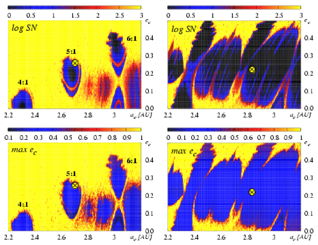
Figure 2.—

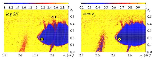
Figure 3.—

Figure 4.—

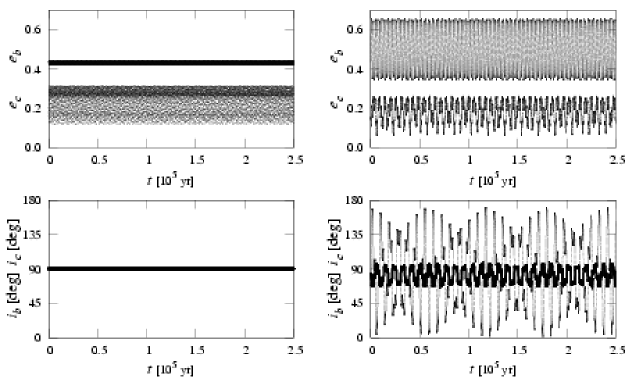
Figure 5.—

Figure 6.—

Figure 7.—

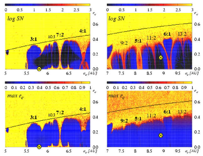
Figure 8.—

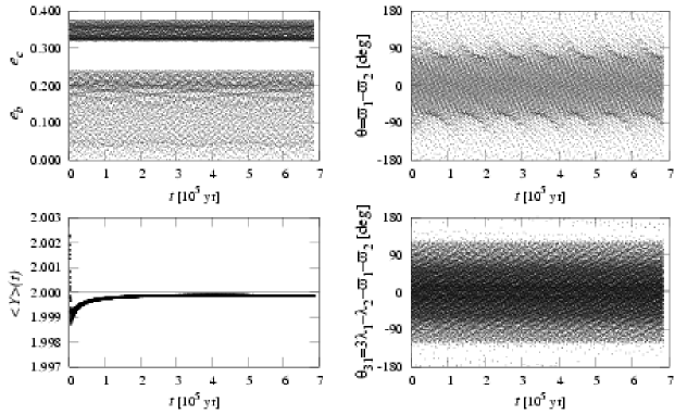
Figure 9.—

Figure 10.—

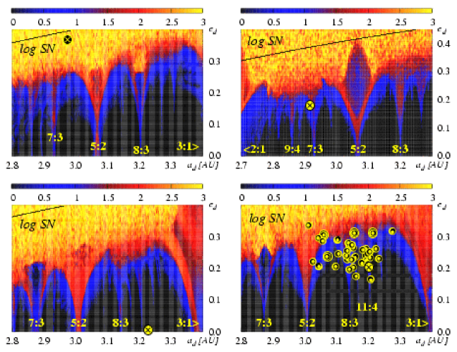
Figure 11.—

Figure 12.—

Figure 13.—

Figure 14.—

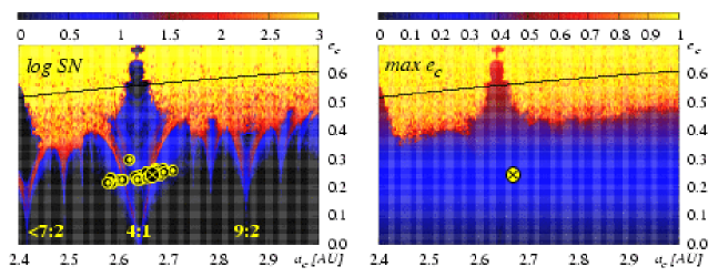
Figure 15.—

Figure 16.—

Figure 17.—

References

- Adams & Laughlin (2003) Adams, F. C. & Laughlin, G. 2003, Icarus, 163, 290
- Arnold (1978) Arnold, V. I. 1978, Mathematical methods of classical mechanics (Graduate texts in mathematics, New York: Springer, 1978)
- Butler et al. (1999) Butler, R. P., Marcy, G. W., Fischer, D. A., Brown, T. M., Contos, A. R., Korzennik, S. G., Nisenson, P., & Noyes, R. W. 1999, ApJ, 526, 916, 1999ApJ…526..916B
- Butler et al. (2003) Butler, R. P., Marcy, G. W., Vogt, S. S., Fischer, D. A., Henry, G. W., Laughlin, G., & Wright, J. T. 2003, ApJ, 582, 455
- Charbonneau (1995) Charbonneau, P. 1995, ApJS, 101, 309
- Cincotta et al. (2003) Cincotta, P. M., Giordano, C. M., & Simó, C. 2003, Physica D, 182, 151
- Cincotta & Simó (2000) Cincotta, P. M. & Simó, C. 2000, A&AS, 147, 205
- Correia et al. (2005) Correia, A. C. M., Udry, S., Mayor, M., Laskar, J., Naef, D., Pepe, F., Queloz, D., & Santos, N. C. 2005, A&A, 440, 751
- Ferraz-Mello et al. (2005) Ferraz-Mello, S., Michtchenko, T. A., & Beaugé, C. 2005, ApJ, 621, 473
- Fischer et al. (2003) Fischer, D. A., Marcy, G. W., Butler, R. P., Vogt, S. S., Henry, G. W., Pourbaix, D., Walp, B., Misch, A. A., & Wright, J. T. 2003, ApJ, 586, 1394
- Ford (2005) Ford, E. B. 2005, Protostars and Planets V, www.lpi.usra.edu/meetings/ppv2005/pdf/8358.pdf
- Giordano & Cincotta (2004) Giordano, C. M. & Cincotta, P. M. 2004, A&A, 423, 745
- Goździewski et al. (2003) Goździewski, K., Konacki, M., & Maciejewski, A. J. 2003, ApJ, 594
- Goździewski et al. (2005) —. 2005, ApJ, 622, 1136
- Goździewski & Maciejewski (2003) Goździewski, K. & Maciejewski, A. J. 2003, ApJ, 586, L153
- Goździewski (2003) Goździewski, K. 2003, A&A, 398, 315
- Gozdziewski & Konacki (2005) Gozdziewski, K. & Konacki, M. 2005, astro-ph/0510109
- Goździewski & Maciejewski (2001) Goździewski, K. & Maciejewski, A. 2001, ApJ, 563, L81
- Jones et al. (2002) Jones, H. R. A., Paul Butler, R., Marcy, G. W., Tinney, C. G., Penny, A. J., McCarthy, C., & Carter, B. D. 2002, MNRAS, 337, 1170
- Laskar (1993) Laskar, J. 1993, Celest. Mech. & Dyn. Astr., 56, 191
- Laughlin & Chambers (2001) Laughlin, G. & Chambers, J. E. 2001, ApJ, 551, L109
- Lecar et al. (2001) Lecar, M., Franklin, F. A., Holman, M. J., & Murray, N. J. 2001, ARA&A, 39, 581
- Lee & Peale (2003) Lee, M. H. & Peale, S. J. 2003, ApJ, 592, 1201
- Lissauer (1999) Lissauer, J. J. 1999, Rev. Mod. Phys., 71, 835
- Marcy et al. (2005) Marcy, G., Butler, R. P., Fischer, D., Vogt, S., Wright, J. T., Tinney, C. G., & Jones, H. R. A. 2005, Progress of Theoretical Physics Supplement, 158, 24
- Marcy et al. (2002) Marcy, G. W., Butler, R. P., , Fischer, D. A., Laughlin, G., Vogt, S. S., Henry, G. W., & Pourbaix, D. 2002, ApJ, submitted
- Mayor et al. (2004) Mayor, M., Udry, S., Naef, D., Pepe, F., Queloz, D., Santos, N. C., & Burnet, M. 2004, A&A, 415, 391
- McCarthy et al. (2004) McCarthy, C. et al. 2004, ApJ
- Michtchenko & Ferraz-Mello (2001) Michtchenko, T. & Ferraz-Mello, S. 2001, ApJ, 122, 474
- Michtchenko & Malhotra (2004) Michtchenko, T. A. & Malhotra, R. 2004, Icarus, 168, 237
- Murray & Dermott (2000) Murray, C. D. & Dermott, S. F. 2000, Solar System Dynamics (Cambridge Univ. Press)
- Naef et al. (2004) Naef, D., Mayor, M., Beuzit, J. L., Perrier, C., Queloz, D., Sivan, J. P., & Udry, S. 2004, A&A, 414, 351
- Pauwels (1983) Pauwels, T. 1983, Celestial Mechanics, 30, 229
- Press et al. (1992) Press, W. H., Teukolsky, S. A., Vetterling, W. T., & Flannery, B. P. 1992, Numerical Recipes in C. The Art of Scientific Computing (Cambridge Univ. Press)
- Thommes & Lissauer (2003) Thommes, E. W. & Lissauer, J. J. 2003, ApJ, 597, 566
- Udry et al. (2002) Udry, S., Mayor, M., Naef, D., Pepe, F., Queloz, D., Santos, N. C., & Burnet, M. 2002, A&A, 390, 267
- Vogt et al. (2005) Vogt, S. S., Butler, R. P. Marcy, G. W., Fischer, D. A., Henry, G. W., Laughlin, G., Wright, J. T., & Johnson, J. A. 2005, ApJ, 1, apJ preprint doi:10.1086/432901
- Wright (2005) Wright, J. T. 2005, PASP, 117, 657