The Tully–Fisher relation of distant field galaxies

Abstract

We examine the evolution of the Tully–Fisher relation (TFR) using a sample of $89$ field spirals for which we have measured confident rotation velocities ($V_{\mathrm{rot}}$). This sample covers the redshift range $0.1\la z\la 1$, with a median of $\left<z\right>=0.33$. The best-fitting TFR has a slope consistent with that measured locally, and we find no significant evidence for a change with redshift, although our sample is not large enough to well constrain this. By plotting the residuals from the local TFR versus redshift, we find evidence that these luminous ($M_{B}\la M^{\ast}_{B}$) spiral galaxies are increasingly offset from the local TFR with redshift, reaching a brightening of $-1.0\pm 0.5$ mag, for a given $V_{\mathrm{rot}}$, by $z\sim 1$. This is supported by fitting the TFR to our data in several redshift bins, suggesting a corresponding brightening of the TFR intercept. Since selection effects would generally increase the fraction of intrinsically-bright galaxies at higher redshifts, we argue that the observed evolution is probably an upper limit.

Previous studies have used an observed correlation between the TFR residuals and $V_{\mathrm{rot}}$ to argue that low mass galaxies have evolved significantly more than those with higher mass. However, we demonstrate that such a correlation may exist purely due to an intrinsic coupling between the $V_{\mathrm{rot}}$ scatter and TFR residuals, acting in combination with the TFR scatter and restrictions on the magnitude range of the data, and therefore it does not necessarily indicate a physical difference in the evolution of galaxies with different $V_{\mathrm{rot}}$.

Finally, if we interpret the luminosity evolution derived from the TFR as due to the evolution of the star formation rate (SFR) in these luminous spiral galaxies, we find that SFR$(z)\propto(1+z)^{1.7\pm 1.1}$. Notwithstanding the relatively large uncertainty, this evolution, which is probably overestimated due to selection effects, seems to be slower than the one derived for the overall field galaxy population. This suggests that the rapid evolution in the SFR density of the universe observed since $z\sim 1$ is not driven by the evolution of the SFR in individual bright spiral galaxies.

1 Introduction

The slope, intercept and scatter of the Tully–Fisher relation (TFR; Tully & Fisher 1977) are key parameters that any successful prescription for galaxy formation and evolution must reproduce. As a relation between the luminosity and rotational velocity of disc galaxies, it is a combination of a number of fundamental galaxy properties and relations. These include the relation between observed rotation velocity and total galaxy mass, that between the total and luminous mass distributions, and the mass-to-light ratio of the galaxy’s stellar population. The first of these is dependent upon the degree to which the stars in the galaxy are rotationally supported and, along with the second relation, is determined by the dynamical galaxy formation process. The third component, the mass-to-light ratio in a particular photometric band, is determined by the star formation history of the galaxy.

The TFR therefore provides a wealth of information about the astrophysical processes involved in forming and maintaining spiral galaxies. In the past decade significant progress has been made toward understanding the origins of the TFR. This involves determining how the parameters involved conspire to maintain the relation, through self-regulation of star-formation in the disk (Silk, 1997), while explaining the variations which lead to its intrinsic scatter. Modern simulations are able to reproduce the slope and scatter of the $I$-band TFR (e.g., Koda et al., 2000), respectively identifying these with the natural range of mass and spin parameters for dark matter haloes. However, reproducing the TFR intercept while matching other properties of the galaxy population is currently beyond the abilities of semi-analytic models (Cole et al., 2000).

As well as a goal to understand in its own right, the TFR is particularly useful as a benchmark with which to compare samples of galaxies, in order to examine the differences between them. Using this method, we can gain insight into the evolution of disc galaxies by considering the variation of the TFR with cosmic time. In this paper we present the $B$-band TFR of field spirals at redshifts $0.1\la z\la 1$, and examine its evolution over the past $8$ Gyr. We then assess the implications of these results for the evolution of the star formation rate (SFR) in spiral galaxies.

In Section 2 we briefly describe our observations, data reduction, and techniques for measuring the galaxy parameters. We present the TFR of our field galaxy sample in Section 3, along with an examination of its evolution with redshift, and a comparison with other studies. This is followed by a discussion of the implications for SFR evolution in Section 4, and finally we give our conclusions in Section 5. Throughout we assume the concordance cosmology, with $\Omega_{\Lambda}=0.7$, $\Omega_{m}=0.3$ and $H_{0}=70$ km s^-1 Mpc^-1. All magnitudes are in the Vega zero-point system.

2 Data

The target selection, photometry and spectroscopy are described thoroughly in Bamford et al. (2005, hereafter Paper I), and therefore only briefly summarized here. The primary motivation for our spectroscopic observations was the comparison of spiral galaxies in five clusters at $0.2\la z\la 0.8$ with field spirals at comparable redshifts. This has been examined in Paper I. In the process we have observed a large number of field galaxies, by themselves forming a useful sample for examining the evolution of the more general spiral galaxy population. This is the subject of the current paper.

2.1 Target selection

For each field, galaxies were identified and their magnitudes measured using SExtractor on our $R$-band imaging. The galaxies to be observed spectroscopically were then selected by assigning priorities based upon the likelihood of being able to measure a rotation curve. Higher priorities were assigned for each of the following: disky morphology, favourable inclination, known emission line spectrum, and available HST data. A priori knowledge of the galaxies’ approximate spectral type varied depending upon the availability of such data in the literature. The following sources were utilized for each field, labelled by the target cluster in that field: MS0440: Gioia et al. 1998; AC114: Couch & Sharples 1987; Couch et al. 1998; A370: Dressler et al. 1999; Smail et al. 1997; CL0054: Dressler et al. 1999; Smail et al. 1997; P-A Duc private comm.; MS1054: van Dokkum et al. 2000. This element of the selection is therefore highly heterogeneous, and certainly not ideal. However, while it makes an understanding of our selection function very difficult, this does reduce the possibility of any systematic effects.

For each spectroscopic mask, slits were added in order of priority, and within each priority level in order from brightest to faintest $R$-band magnitude. The only reason for a particular galaxy not being included is a geometric constraint caused by a galaxy of higher priority level, or a brighter galaxy in the same priority level. Often the vast majority of the mask was filled with slits on galaxies in the highest priority levels, with occasional recourse to lower priority objects in order to fill otherwise unoccupied gaps in the mask. The redshift distribution of our field sample is shown in Fig. 1.

Figure 1: The redshift distribution of our target galaxies. The hatched histogram shows the distribution of all field galaxies observed with identifiable emission lines, and the filled area only those in our final TFR field sample.

2.2 Photometry

The photometry for this study was principally measured on HST archive images, supplemented by our own FORS2 (Seifert et al., 2000) $R$-band imaging and additional ground-based data, kindly provided by Dr. Ian Smail. These latter images provide additional colour information, improving the $k$-correction by helping constrain the galaxy SED. The magnitudes used in this paper are measured within SExtractor AUTO (Kron-style) apertures (Bertin & Arnouts, 1996), and are corrected for Galactic extinction using the maps and conversions of Schlegel, Finkbeiner & Davis (1998).

The observed apparent magnitudes were converted to apparent rest-frame $B$-band magnitudes by a colour- and $k$-correction, determined using the observed colour information where available and the SEDs of Aragón-Salamanca et al. (1993). The absolute rest-frame $B$-band magnitudes were then obtained assuming the concordance cosmology. Finally the magnitudes were corrected for internal extinction (including face-on extinction of $0.27$ mag), following the prescription of Tully & Fouque (1985), to give the corrected absolute rest-frame $B$-band magnitudes, $M_{B}$, used in the following analysis. Note that both the cosmology and internal extinction correction prescription were chosen to allow straightforward comparison with other recent studies.

Figure 2: Absolute rest-frame $B$-band magnitude versus redshift for all our field galaxies with identifiable emission lines. Galaxies in our final field TFR sample are shown by filled points, while open points indicate those for which no emission lines pass our quality control criteria (see Section 2.3). The dashed line indicates $M^{\ast}_{B}$ as calculated in the text. The dotted line shows the absolute magnitude corresponding to an apparent rest-frame $B$-band magnitude of $22.5$ mag, as a function of redshift in our adopted cosmology.

A plot of $M_{B}$ versus redshift is shown in Fig. 2. Notice how our sample is limited to brighter brighter magnitudes with increasing redshift. We can assess how much of the typical galaxy population we sample by comparing with the $M^{\ast}$ luminosity function parameter. Norberg et al. (2002) use data from the 2dF Galaxy Redshift Survey to measure the $b_{J}$-band luminosity function, finding $M^{\ast}_{b_{J}}-5\log(h)=-19.66\pm 0.07$ mag. We can transform this into the $B$-band using the conversion suggested by Norberg et al. (2002), $b_{J}=B-0.28(B-V)$, and the colour of a typical galaxy in our sample (estimated from the best-fitting SEDs), $(B-V)=0.52$. With $H_{0}=70$ km s^-1 Mpc^-1, we therefore have $M^{\ast}_{B}\simeq-20.3$ mag. This is shown by the dashed line in Fig. 2. At $z\sim 0.2$ we sample a range $\sim\!2$ mag either side of $M^{\ast}_{B}$. By $z\sim 0.5$ this has reduced to $(M^{\ast}_{B}-2)\la M_{B}\la M^{\ast}_{B}$ mag, and at $z\sim 0.8$ we are limited to $M_{B}\la(M^{\ast}_{B}-1)$ mag. We therefore sample most of the giant spiral population below $z\sim 0.5$, but beyond this we are limited to only the brightest galaxies in this class. Note that this effect is less serious than in conventional magnitude limited studies as our galaxies at high redshifts have, on average, been observed with longer spectroscopic integrations. This is because the majority of our high-redshift galaxies are from masks targeting our more distant clusters, and thus with longer exposure times (see Section 2.3).

Inclinations ($i$) and photometric scalelengths ($r_{\mathrm{d,phot}}$) for the disk components of the observed galaxies were measured in bands close to $R$, preferentially in the HST images (bands F606W, F675W or F702W), and primarily using gim2d (Simard et al., 2002). Reliable HST inclination (scalelength) measurements were available for $47$ ($39$) per cent of the galaxies; for the remainder inclination (scalelength) was measured on the ground-based $R$-band imaging, again usually by gim2d. These measurements are therefore separated from the effect of the bulge component and corrected for the effect of seeing. For a small number of galaxies the gim2d fit was unreliable. In these cases the SExtractor axial ratio was used, assuming an infinitely thin disk (as does gim2d). These inclinations were corrected by a factor determined from an empirical comparison of SExtractor and gim2d based inclinations. One factor was used for all ground-based measurements, and another for the HST measurements.

In order to further evaluate our selection function, we measure effective radii, $r_{\mathrm{eff}}$, of circular apertures containing half the galaxy light. These were obtained from our FORS2 $R$-band imaging, the only band which is available for nearly all of our galaxies, using SExtractor’s FLUX_RADIUS output. Plots of $r_{\mathrm{d,phot}}$ and $r_{\mathrm{eff}}$ versus redshift are shown in Fig. 3. Both of these plots include a dotted curve indicating the physical size, in kpc, corresponding to an observed angle of $1$ arcsec, as a function of redshift. The seeing in the $R$-band imaging is roughly $1$ arcsec FWHM, but for comparison with $r_{\mathrm{eff}}$ one must convert this to a half-light radius. A Gaussian profile with $1$ arcsec FWHM has a half-light radius of $\sim\!0.6$ arcsec. The measured $r_{\mathrm{eff}}$ are thus all larger than the seeing, but from the correlation of the lower bound of the points $r_{\mathrm{eff}}$ distribution with redshift, the seeing is often dominating the measurement.

In order to compare the seeing scale with $r_{\mathrm{d,phot}}$ one can note that if the exponential scalelength of a point source, with a Gaussian seeing profile, were measured, the result would be close to the radius at which a Gaussian profile reaches $1/e$ of its peak value. This occurs at a radius of $0.6$ times the FWHM. However, this comparison is complicated by the inclusion of a bulge component in the fit surface brightness model. To some extent, though, the fact that the $r_{\mathrm{d,phot}}$ distribution extends below the seeing scale, and shows little variation in its lower limit with redshift, indicates that $r_{\mathrm{d,phot}}$ is rather more independent of the seeing.

However, due to the similarity of the galaxy sizes to the seeing scale, and in particular the impact of limited resolution on the bulge-disc decomposition, our disc scalelengths are potentially unreliable. This problem becomes significantly worse for both higher redshift and intrinsically smaller galaxies. We therefore choose not to base any inferences on our measurements of galaxy size, and only use them to give an indication of any biases in our sample selection.

Figure 3: Plots against redshift of (a) photometric disc scalelength, $r_{\mathrm{d,spec}}$ and (b) effective (half-light) radius, $r_{\mathrm{eff}}$, both in kpc, for all our field galaxies with identifiable emission lines (excluding the supplementary MS1054 field in panel (b)). Galaxies in our final field TFR sample are shown by filled points, while open points indicate those for which no emission lines pass our quality control criteria (see Section 2.3). The dotted line indicates the physical size subtended by an angle of $1$ arcsec, as a function of redshift in our adopted cosmology. The dashed line in panel (b) shows the same for an angle of $0.6$ arcsec, approximately equal to both the half-light radius and exponential scalelength of a Gaussian with $1$ arcsec FWHM.

Another tool to examine our sample selection is provided by the surface brightness of our galaxies. We calculate the apparent $R$-band average surface brightness within $r_{\mathrm{eff}}$, which we denote $\mu_{R,\mathrm{eff},\mathrm{app}}$, using $\mu_{R,\mathrm{eff},\mathrm{app}}=R_{\mathrm{eff}}+2.5\log{2\pi r_{\mathrm{eff}}^{2}}$, where $R_{\mathrm{eff}}=R+2.5\log{2}$ is the magnitude within $r_{\mathrm{eff}}$ by the definition of the half-light radius, with total magnitude, $R$. This, converted into an absolute observed-frame $R$-band surface brightness using the distance modulus for our adopted cosmology (denoted $\mu_{R,\mathrm{eff},\mathrm{abs}}$), is plotted in Fig. 4.

Figure 4: Plot against redshift of the absolute observed-frame $R$-band surface brightness within $r_{\mathrm{eff}}$, for all our field galaxies with identifiable emission lines (excluding the supplementary MS1054 field). Galaxies in our final field TFR sample are shown by filled points, while open points indicate those for which no emission lines pass our quality control criteria (see Section 2.3). The dotted line indicates the absolute surface brightness corresponding to an observed apparent surface brightness of $25$ mag arcsec^-1, according to our adopted cosmology.

A comparison of Figs. 2 and 4 reveals the two plots to show very similar behaviour. This, along with the apparent lack of any redshift-dependent selection on $r_{\mathrm{d,phot}}$ demonstrated by Fig. 3(a), and the simple explanation that the correlation in Fig. 3(b) is due to seeing affecting the $r_{\mathrm{eff}}$ measurement, rather than any selection effect, implies that the surface brightness distribution is largely a result of a magnitude-limited selection, rather than any selection on galaxy size.

The distributions in all these plots of the galaxies which make our final TFR sample, relative to those in the whole sample, are considered in the following section, after a description of the final TFR sample selection criteria.

2.3 Spectroscopy

The spectroscopy for this study was observed using FORS2 (Seifert et al., 2000), in MXU mode, on the VLT. In this mode, multiple slits are cut into a mask which is placed in the focal plane. The slits were individually tilted to align with the major axis of each galaxy, as determined from the $R$-band pre-imaging. Slits of 1 arcsec width in the dispersion direction were used, with lengths that varied in order to sample sky at the edge of each galaxy, while efficiently packing the masks with targets. Exposure times varied from $30$ to $210$ minutes per mask, depending on the redshift of the cluster that formed the primary target for each observation. The seeing was typically $\sim\!1$ arcsec and always below $1.2$ arcsec. These data and their reduction are described more completely in Paper I, and are therefore only briefly summarised here.

The data were reduced in the usual manner (Milvang-Jensen 2003; Bamford thesis in preparation) to produce straightened, flat-fielded, wavelength-calibrated and sky-subtracted 2d-spectra for each galaxy. From these, individual sky- and continuum-subtracted emission line ‘postage stamps’ were extracted. The main emission lines observed were [OII]$\lambda 3727$, H$\beta$ and [OIII]$\lambda\lambda 4959,5007$, with H$\alpha$ but no [OII]$\lambda 3727$ for nearby galaxies ($z\la 0.3$, depending upon the position of the slit in the mask). In order to measure the rotation velocity ($V_{\mathrm{rot}}$) and emission scale lengths ($r_{\mathrm{d,spec}}$) we fit each emission line independently using a synthetic rotation curve method based on elfit2d by Simard & Pritchet (1998, 1999), and dubbed elfit2py. In this technique a model emission line is created for particular sets of parameters, assuming a form for the intrinsic rotation curve, an exponential surface-brightness profile, and given the galaxy inclination, seeing and instrumental profile. The intrinsic rotation curve assumed here is the ‘universal rotation curve’ (URC) of Persic & Salucci (1991), with a slope weakly parametrized by the absolute $B$-band magnitude, $M_{B}$. From a comparison of the results from fits using both flat and ‘universal’ intrinsic rotation curves, adopting a flat rotation curve leads to values of $V_{\mathrm{rot}}$ $\sim\!10$ km s^-1 lower than found with the URC. The choice of rotation curve does not appear to affect the conclusions of this study. A Metropolis algorithm is used to search the parameter space to find those which best fit the data, and to determine confidence intervals on these parameters. Images of model lines with the best-fitting parameters are also produced for comparison with the data.

In order to produce a single value of $V_{\mathrm{rot}}$ and $r_{\mathrm{d,spec}}$ for each galaxy, the values for the individual lines are combined by a weighted mean, as described in Paper I.

A significant fraction of the emission lines identified display dominant nuclear emission, or asymmetries in intensity, spatial extent or kinematics. In severe cases these departures from the assumed surface brightness profile and intrinsic rotation curve mean that the best-fitting model is not a true good fit to the data. A similar situation can occur for very low signal-to-noise ($S\!\left/N\right.$) lines, where an artifact of the noise overly influences the fit. More concerning is the case of very compact lines, where the number of pixels is on the order of the number of degrees of freedom in the model, and hence an apparently good fit is obtained despite a potentially substantial departure from the assumed surface brightness profile.

In order to eliminate such ‘bad’ fits a number of quality tests are imposed, based on a measure of the median $S\!\left/N\right.$ and a robust $\chi^{2}$ goodness-of-fit estimate. In addition, the emission lines were ‘traced’ by fitting a Gaussian to each spatial column of pixels, and the region determined for which the trace is reliable. The distance from the continuum centre to where the line could no longer be reliably detected above the noise we term the extent. Additionally, quantities describing the asymmetry, in terms of extent and kinematics, and the flatness of the line at maximum extent were formulated. Unfortunately, a satisfactory set of quantitative criteria, to exclude ‘bad’ fits while efficiently retaining ‘good’ fits, could not be found. Therefore, we supplemented cuts on $S\!\left/N\right.$and $\chi^{2}$ with a visual inspection of every emission line, supported by the various quality tests just described. In the process galaxies with apparently dominant nuclear emission were excluded, as were lines producing zero $V_{\mathrm{rot}}$ estimates and those clearly inconsistent with a number of other lines for the same galaxy.

As in Paper I, we have supplemented our data with that from Milvang-Jensen et al. (2003). This is also FORS2 MXU data, reduced in a very similar way to that described above. In order to consistently combine the MS1054 data with this sample, the emission line postage stamps for the MS1054 galaxies have been re-fit using elfit2py and the same line quality criteria applied.

After all these quality checks, our full field galaxy TFR sample contains $89$ galaxies, with a mean of $\sim\!2.3$ emission lines contributing to the measurements for each galaxy. This sample covers the redshift range $0.1\la z\la 1$, with a median redshift of $\left<z\right>=0.33$, as show in Fig. 1.

Figures 2, 3 and 4 show the distributions of $M_{B}$, $r_{\mathrm{d,phot}}$, $r_{\mathrm{eff}}$ and $\mu_{R,\mathrm{eff},\mathrm{abs}}$ versus redshift for all field emission line galaxies observed. Those in our final TFR sample are marked by filled points, while those which are not, i.e., for which none of the emission line fits passed our quality criteria, are shown by open points. There is no noticeable difference between the distributions of selected and rejected galaxies in these plots. This indicates that our quality selection criteria are not biasing our sample from the point of view of the galaxies’ broadband photometric properties, beyond those baises inherent to our initial spectroscopy observational selection procedure.

3 The Tully–Fisher relation

3.1 Basic fit

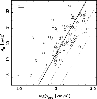
Figure 5: The Tully–Fisher relation for our full field TFR sample. The fiducial local relation of Pierce & Tully (1992) is marked by the dot-dashed line, with its $3\sigma$ intrinsic scatter delimited by dotted lines. A weighted least-squares fit to all the points is shown by the solid line, see the text for details. The error bars in the top left corner indicate the 10th-, 50th- and 90th-percentiles of the (broadly unimodal) distribution of uncertainties on the displayed points.

Our TFR for distant field galaxies is given in Fig. 5. The solid line is an ‘inverse’ fit to the data,

$$\log{V_{\mathrm{rot}}}=a+bM_{B}$$ (1)

found by minimising the weighted squared deviations in $\log{V_{\mathrm{rot}}}$. The weights applied to each point are

$$w_{i}=1\!\left/\sigma_{i}^{2}\right.\;,$$ (2)

where

$$\sigma_{i}^{2}=\sigma_{\log{V_{\mathrm{rot}}},i}^{2}+b^{2}\sigma_{M_{B},i}^{2}+\sigma_{\mathrm{int}}^{2}\;.$$ (3)

Here $\sigma_{\log{V_{\mathrm{rot}}},i}$ and $\sigma_{M_{B},i}$ are the errors on each point derived from the reduction process, and $\sigma_{\mathrm{int}}$ is the intrinsic scatter of the TFR, which is allowed to vary such that the reduced chi-squared statistic, $\chi_{\mathrm{r}}^{2}$, is unity. This was achieved by iteration, each time recalculating the weights using the new value of $b$, and $\sigma_{\mathrm{int}}$ determined via the recurrence relation

$$\sigma_{\mathrm{int},{j+1}}^{2}=\sigma_{\mathrm{int},{j}}^{2}\,\chi_{\mathrm{r}}^{2\alpha}\;;\quad\mathrm{with}\ \alpha>0\;,$$ (4)

where, as usual for two degrees of freedom, the reduced-chi-squared statistic is

$$\chi_{\mathrm{r}}^{2}=\frac{\chi^{2}}{n-2}\;,\quad\chi^{2}=\sum_{i}{\left(\frac{\log{V_{\mathrm{rot}}}_{i}-a-bM_{B,i}}{\sigma_{i}}\right)^{2}}\;.$$ (5)

The (weighted) total scatter, $\sigma_{\mathrm{total}}$, is calculated by

$$\sigma_{\mathrm{total}}^{2}=\sum_{i}{w_{i}\left(\log{V_{\mathrm{rot}}}_{i}-a-bM_{B,i}\right)^{2}}\left/\sum_{i}{w_{i}}\right.\;.$$ (6)

Notice that when $\chi_{\mathrm{r}}^{2}$ is at the desired value of unity, the $\sigma_{\mathrm{int}}^{2}$ recurrence relation (Eqn. 4) reduces to $\sigma_{\mathrm{int},{j+1}}^{2}=\sigma_{\mathrm{int},{j}}^{2}$, as we would want. When $\chi_{\mathrm{r}}^{2}>1$ this implies $\sigma_{\mathrm{int}}^{2}$ is too small, and thus it is increased for the next iteration. Alternatively, when $\chi_{\mathrm{r}}^{2}<1$ this implies $\sigma_{\mathrm{int}}^{2}$ is too large, and it is therefore decreased for the next iteration. The value of $\alpha$ may be tuned to minimise the number of iterations before convergence is achieved; $\alpha=\frac{2}{3}$ was found to work well.

The fit converges in $\sim\!4$ iterations to give the TFR (converted back into the ‘forward’ form):

$$M_{B}=(-8.1\pm 0.8)\cdot\log{V_{\mathrm{rot}}}\>+\>(-3.2\pm 2.0)$$ (7)

with $\sigma_{\mathrm{total}}=1.0$ mag and $\sigma_{\mathrm{int}}=0.9$ mag.

The ‘inverse’ fit is often used to avoid a potential bias because of the apparent magnitude limited nature of a TFR sample. At faint apparent magnitudes, points are preferentially selected above the real TFR. For samples over a narrow range of distance moduli, e.g., in local cluster studies, the nature of this bias is to cause an apparent flattening of the TFR slope. While the dependence of $V_{\mathrm{rot}}$ on $M_{B}$ still causes an effect, Willick (1994) has shown that using an ‘inverse’ fit reduces the bias by a factor of five compared with the conventional ‘forward’ fit. As this study covers a wide range of distance moduli, apparently faint galaxies are found over the whole range of absolute magnitude, depending on their redshift. Any bias on the best-fitting TFR should therefore be weakened, and take the form of an intercept shift rather than a flattening of the slope. This is particularly true given the more random priority-based, rather than magnitude-based, selection. However, to minimise any such effect, and allow us to confidently use the same fitting method to compare differently selected samples, we choose to work with the ‘inverse’ fit.

We weight our fit to make full use of the data, and avoid the influence of unreliable points, while the inclusion of an intrinsic scatter term prevents points with small errors from dominating the fit, and allows us to estimate this useful parameter.

The thin lines in Fig. 5 indicate a fiducial local field TFR. This is derived from the TFR of Pierce & Tully (1992, hereafter PT92), with a zero-point adjustment because PT92, while otherwise using the internal extinction correction of Tully & Fouque (1985), do not include the $0.27$ mag of face-on extinction that is applied to our data. The fiducial PT92 TFR, adapted to our internal extinction correction, is thus:

$$M_{B}^{\mathrm{PT92}}(V_{\mathrm{rot}})=-7.48\log{V_{\mathrm{rot}}}-3.37\;.$$ (8)

PT92 obtained this relation by an ‘inverse’ least-squares fit, minimising the residuals in rotation velocity. This is the same method we have used to fit our TFR, except that our fit is weighted and includes the intrinsic scatter in these weights. The weighting should not cause any bias, and hence our fitting method is comparable to that used to produce the fiducial TFR of PT92.

There is clearly a significant offset between the TFRs of PT92 and this study. This may not be entirely an evolutionary effect, and some part of it is likely due to the different manner in which we measure the rotation velocities and magnitudes compared with PT92. Note that in generating the fiducial relation we have assumed that $V_{\mathrm{rot}}=0.5W^{i}_{R}$, where $W^{i}_{R}$ is the fully-corrected HI velocity width measured by PT92.

A further issue is whether or not the absolute calibration of the PT92 TFR is correct. This is based upon Cepheid and RR Lyrae distances to six local calibrator galaxies, and hence dependent upon the calibration of the whole extra-galactic distance scale at the time. There is also the issue of how representative this small number of local calibrator galaxies are compared with the whole PT92 TFR sample. Pierce (1994, hereafter P94) uses the PT92 TFR to calibrate supernovae distances and derive $H_{0}=86\pm 7$ km s^-1 Mpc^-1. If, as is suggested, the primary cause of uncertainty in this value is the absolute TFR calibration, then we could potentially use the modern, significantly more accurate value of $H_{0}$ to correct this. We could therefore derive a more accurate TFR absolute calibration by using our cosmologically measured $H_{0}$, a reversal of the traditional method.

The current best estimate of $H_{0}$ is provided by a combination of data from WMAP and a number of other surveys: $H_{0}=71$$-3$$+$$-$$4$ km s^-1 Mpc^-1 (Spergel et al., 2003). The difference in distance modulus between this $H_{0}$ and that derived by P94 is $0.5\pm 0.1$ mag, in the sense of moving the TFR to brighter magnitudes. The errors given only include those on the WMAP $H_{0}$ measurement, as the P94 errors are dominated by the uncertainty on the distance scale, which we are replacing. It can therefore be argued that a correction of $-0.5$ mag should be applied to the intercept of the PT92 TFR.

Fortunately in this study the uncertainty on the intercept of the fiducial local TFR is of little concern. Our sample covers a wide range in redshift, selected and analysed in a homogeneous manner. We can therefore examine the TFR evolution using only this study’s data, without recourse to external work.

In future studies it may be wise to consider using the more recent $B$-band TFR of Tully & Pierce (2000) as a comparison. This relation has an absolute calibration based on Cepheid distances to $24$ galaxies and implies a value of $H_{0}=77\pm 8$, more consistent with the WMAP result. The work of Verheijen (2001) provides another more recent local comparison TFR, which has already been used by some groups. However, these studies use the internal extinction correction scheme of Tully et al. (1998), which has a strong dependency upon galaxy luminosity (or alternatively $V_{\mathrm{rot}}$). While this form of the internal extinction should be more accurate, it will require care as the dependency on luminosity (or $V_{\mathrm{rot}}$) is calibrated locally, and may not be valid for distant galaxies.

The internal scatter we measure, $\sigma_{\mathrm{int}}=0.90$ mag, is considerably larger than the $\sim 0.4$ mag generally found for local samples (e.g Pierce & Tully, 1992; Dale et al., 1999). However, most local studies are focused upon using the TFR as a distance indicator. They therefore impose very strict selection criteria, e.g., requiring undisturbed late-type spirals, in an effort to produce as strong a correlation as possible. At high redshift we do not have the luxury of abundant data, and so cannot impose such strict criteria. For example, it is harder to identify galaxies with slightly disturbed rotation curves and morphologies, making rejection of such objects impossible. In addition, corrections for known, locally-calibrated correlations, e.g., between TFR intercept and morphological type, are often applied to local samples. However, such corrections are not yet calibrated at high-redshift and so cannot be applied to our data. The variations caused by minor disturbances, differing sample selection, and varying corrections may be responsible for the entire increase in intrinsic scatter. However, physical effects, such as an increased stochasticity of star-formation, may also contribute.

3.2 TFR evolution with redshift

The slope of the TFR we measure for the whole field galaxy sample is very similar to that found locally by PT92, and consistent within our errors. Note that we have used a comparable fitting method to PT92, so this statement is valid. The precise slope measured is very much dependent on the fitting method employed, and may explain why some studies find apparently different slopes. Our fit suggests there is little change in the TFR slope with redshift. We can attempt to evaluate this further by fitting redshift sub-samples of our data.

As noted above, any difference in intercept between our sample and the local relation of PT92 may not be a real effect. However, by fitting redshift sub-samples we may investigate any evolution of this offset purely within our own sample.

Figure 6: Plots showing the evolution of the slope and intercept of the best-fitting TFR in several redshift bins, indicated by the horizontal error bars. Panel (a) gives the intercept (at the median $V_{\mathrm{rot}}$ of the full sample) for TFR fits to five redshift subsamples of the data. Each redshift bin contains $\sim\!18$ points. The line shows a weighted least-squares fit to the points. For these fits the slope was held fixed to the PT92 value. Panel (b) plots the slope for TFR fits to three redshift subsamples of the data. Each redshift bin contains $\sim\!30$ points. The horizontal lines show the local TFR slope of PT92 (dotted) and the slope from Eqn. 7, the fit to our whole field TFR sample (dashed).

In order to examine the intercept evolution we divide the sample in to five bins, each of $18$ points ($17$ for the highest redshift bin). The TFR is fit for each bin using the usual method, but with the slope constrained to the PT92 value (and hence very similar to the value for our whole sample) to isolate the changes in intercept. In panel (a) of Fig. 6 we plot these results, as the $M_{B}$ value of the best-fitting TFR at the median $V_{\mathrm{rot}}$ of the full sample. Also plotted is a conventional weighted least-squares fit to the points. There is reasonably clear evidence for a brightening of the TFR intercept with redshift of $\sim\!1$ mag by $z=1$, corresponding to a factor of $\sim\!2.5$ in luminosity at a fixed rotation velocity.

At high redshift, however, we only sample the bright end of the galaxy luminosity function, and hence preferentially select objects which have been brightened. In particular we require a certain emission line flux to measure $V_{\mathrm{rot}}$, and hence the limiting emission line luminosity of our sample will increase with redshift. As emission line luminosity increases with SFR, we will therefore sample galaxies with higher SFR at higher redshifts, which in turn implies brighter $B$-band magnitudes for the high-redshift galaxies. The evolution of the TFR intercept that we measure is therefore probably an upper limit on the true brightening, e.g., at a given galaxy mass.

To investigate any evolution in the TFR slope we divide the full sample into only three redshift bins, as the slope requires more points to constrain it. Each bin thus contains 30 points (29 for the highest redshift bin). A TFR was fit to each sub-sample in the same way as for the full sample, and the results are shown in panel (b) of Fig. 6. Due to the small numbers of points in each bin, the errors on the slope are quite large. Given these errors, and the restricted $M_{B}$ range of the data in the highest redshift bin, no strong constraints can be inferred. However, the slope in each bin is consistent with no evolution of this parameter with redshift.

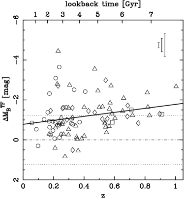
Figure 7: The residuals, $\Delta{M_{B}}^{\!\mathrm{TF}}$, from the fiducial PT92 TFR plotted against redshift and look-back time. Galaxies with $\mu_{R,\mathrm{eff},\mathrm{abs}}<-20.0$ are denoted by squares, those with $-20.0<\mu_{R,\mathrm{eff},\mathrm{abs}}<-18.0$ are shown by triangles, circles denote those with $\mu_{R,\mathrm{eff},\mathrm{abs}}>-18.0$, and galaxies with no $\mu_{R,\mathrm{eff},\mathrm{abs}}$ measurement (i.e., those from the supplementary MS1054 data) are indicated by diamonds. The fiducial local relation of PT92 is again marked by the thin dot-dashed and dotted lines. A weighted least-squares fit to all the points is shown by the solid line, see the text for details. The error bars in the top left corner indicate the 10th-, 50th- and 90th-percentiles of the (broadly unimodal) distribution of uncertainties on the displayed points.

In order to further investigate changes in the intercept of the TFR via the offsets of individual galaxies, it is helpful to work with the residuals from the fiducial TFR:

$$\Delta{M_{B}}^{\!\mathrm{TF}} = M_{B}-M_{B}^{\mathrm{PT92}}(V_{\mathrm{rot}})$$ (9)

$$= M_{B}-\left(-7.48\log{V_{\mathrm{rot}}}-3.37\right)\;.$$

We can evaluate an evolution of the TFR with redshift by looking at a plot of these residuals versus redshift, as shown in Fig. 7. A trend in $\Delta{M_{B}}^{\!\mathrm{TF}}$ with redshift, such that more distant galaxies are brighter for a given rotation velocity, is apparent. Fitting the data in a similar manner to that described for the TFR in Section 3.1 (minimising residuals in $\Delta{M_{B}}^{\!\mathrm{TF}}$) produces the relation

$$\Delta{M_{B}}^{\!\mathrm{TF}}=(-1.0\pm 0.5)\cdot z+(0.8\pm 0.2)\ \mathrm{mag}$$ (10)

with $\sigma_{\mathrm{total}}=0.9$ mag and $\sigma_{\mathrm{int}}=0.8$ mag. This is in good agreement with the more qualitative result from Fig. 6. Once again, however, this is most likely an upper limit on the true luminosity evolution experienced by giant spirals in the field, due to our preferential selection of the brightest objects at high redshift.

In Fig. 7 there is clearly some asymmetric scatter to brighter offsets, which decreases with redshift. This may be due, at least in part, to the fact that there is a larger scatter in the TFR around $V_{\mathrm{rot}}\sim 100$ km s^-1. Only brighter galaxies, and hence those with $V_{\mathrm{rot}}\ga 150$ km s^-1 and thus lower TFR scatter, are observed at high redshifts. However, this does not seem able to account for the whole effect, and there is a hint that this reduction in scatter with redshift is real.

The points in Fig. 7 are shown using different symbols depending upon absolute surface brightness, $\mu_{R,\mathrm{eff},\mathrm{abs}}$. There appears to be no obvious difference in the $\Delta{M_{B}}^{\!\mathrm{TF}}$ distribution of high and low surface brightness galaxies at a given redshift. This argues against the variation in scatter being simply a consequence of sampling different surface brightness ranges at different redshifts. It also implies that the varying surface brightness selection function has relatively small impact on the evolution we measure.

As mentioned in the previous section, there is a systematic offset between our TFR and that of PT92, even when the evolution with redshift is taken into account (as indicated by the zero-point of Eqn. 10 being inconsistent with zero). The earlier discussion of the uncertainties in the intercept of the PT92 TFR also applies here. Note that the ‘cosmological’ correction of $-0.5$ mag suggested in Section 3.1 would bring the zero-points into much closer agreement. In addition, there are a variety of other possible explanations for the offset. For example, the asymmetric scatter to brighter $M_{B}$ for a given $V_{\mathrm{rot}}$, seen particularly at lower redshifts, may influence the fit away from the PT92 relation. This scatter may be due to galaxies that would not have been included in the PT92 sample, for example due to interactions, or that are less prevalent locally. A more rapid evolution in the past $\sim\!2$ Gyr, which is not well constrained by our data, could also be responsible.

3.3 TFR residuals versus $\mn@boldsymbol{V_{\mathrm{rot}}}$

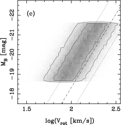
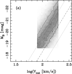
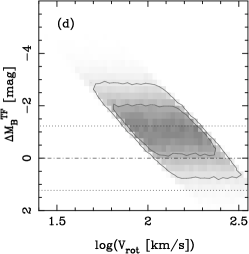
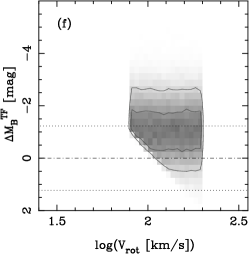
Figure 8: A simple demonstration of the intrinsic correlation between the TFR residuals from the fiducial PT92 TFR, ie., $\Delta{M_{B}}^{\!\mathrm{TF}}$, and $V_{\mathrm{rot}}$. The fiducial local relation of PT92 is again marked by the thin dot-dashed and dotted lines. Panels (a) and (b) show instructive diagrams of the TFR and $\Delta{M_{B}}^{\!\mathrm{TF}}$ versus $\log{V_{\mathrm{rot}}}$ plot, respectively. Each line in panel (b) corresponds to the same style of line in panel (a). Panels (c) and (d) show the distribution of points, as greyscale and contours, for simulated galaxies with true $\log(V_{\mathrm{rot}})$ uniformly distributed on the range $1.9$–$2.3$, true $M_{B}$ assigned to each galaxy corresponding to the PT92 TFR, with a constant offset to make it more easily comparable to our intermediate redshift data. Gaussian scatter with 0.133 dex standard deviation (corresponding to 1.0 mag in terms of $M_{B}$ assuming the PT92 TFR slope) has been added to generate the observed $\log{V_{\mathrm{rot}}}$. No scatter is added to the $M_{B}$ values. Panels (e) and (f) show the distribution of simulated galaxies with true properties created in the same manner as the previous panels. However, in generating the observed values in this case, no scatter has been added to $\log{V_{\mathrm{rot}}}$, while Gaussian scatter with 1.0 mag standard deviation is added to the $M_{B}$. In addition, to demonstrate the effect of a magnitude cut, points with observed $M_{B}>-18.64$ have been removed from the sample. See the text for a more detailed discussion.

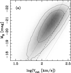
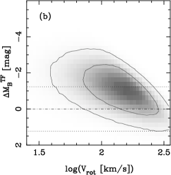
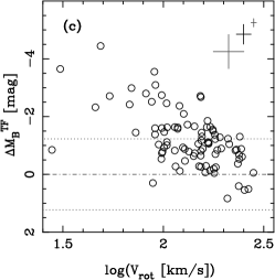
Figure 9: A more detailed demonstration of the intrinsic correlation between $\Delta{M_{B}}^{\!\mathrm{TF}}$ and $V_{\mathrm{rot}}$. The fiducial local relation of PT92 is again marked by the thin dot-dashed and dotted lines. Panels (a) and (b) show the distribution of points in the TFR and $\Delta{M_{B}}^{\!\mathrm{TF}}$ versus $\log{V_{\mathrm{rot}}}$ plot, respectively, for a realistic simulated sample of galaxies, as described in the text. This may be compared with panel (c), a plot of $\Delta{M_{B}}^{\!\mathrm{TF}}$ versus $\log{V_{\mathrm{rot}}}$ for our real field TFR sample. Note the clear correlation, which, as shown by the simulations, may be explained purely by the intrinsic correlation between $\Delta{M_{B}}^{\!\mathrm{TF}}$ and $\log{V_{\mathrm{rot}}}$, along with the effect of scatter in the TFR combined with a restriction on the magnitude range of the data. This correlation, therefore, does not necessarily imply that the data prefers a slope of the TFR different to that of the chosen fiducial TFR, and is thus not adequate evidence for such a real, physical effect.

It may be thought that plotting the TFR residuals, $\Delta{M_{B}}^{\!\mathrm{TF}}$, versus $V_{\mathrm{rot}}$ would provide a test for a change of slope. However, this must be treated very carefully, as the two variables are intrinsically correlated through the scatter in $V_{\mathrm{rot}}$. Böhm et al. (2004, hereafter B04) use this plot to argue that galaxies with lower $V_{\mathrm{rot}}$, and hence lower mass, are offset further from the local TFR than more massive galaxies. However, a correlation between $\Delta{M_{B}}^{\!\mathrm{TF}}$ and $V_{\mathrm{rot}}$ does not necessarily imply such a result. The fact that the two variables are not independent (cf. Eqn. 9), combined with scatter in the TFR and restrictions on the magnitude range of the data, causes an intrinsic correlation, even in the absence of any true difference in TFR slope.

In order to show this in more detail, Fig. 8 gives a pedagogical illustration of the effect of scatter and magnitude cuts on the distribution of points in the TFR and $\Delta{M_{B}}^{\!\mathrm{TF}}\!\!$ – $\log{V_{\mathrm{rot}}}$ plots. Panels (a) and (b) show three corresponding lines in the TFR and $\Delta{M_{B}}^{\!\mathrm{TF}}\!\!$ – $\log{V_{\mathrm{rot}}}$ plot, respectively. The thick solid line is an example ideal TFR, corresponding to the PT92 relation with a constant magnitude offset of $-1.06$ mag, the median $\Delta{M_{B}}^{\!\mathrm{TF}}$ of our data, in order to allow more direct comparison of the examples with our data. This example TFR is limited to the range $1.9<\log{V_{\mathrm{rot}}}<2.3$, and hence $-18.64>M_{B}>-21.63$. The thick dashed and dotted lines indicate loci of constant $M_{B}$ at the faint and bright limits of the example TFR, respectively. In panel (b), the plot of $\Delta{M_{B}}^{\!\mathrm{TF}}$ versus $\log{V_{\mathrm{rot}}}$, the example TFR becomes a (relatively short) horizontal line, while the loci of constant $M_{B}$ are lines with a slope negative that of the example TFR, as is obvious from consideration of Eqn. 9.

To show the transformation of distributions of points in the TFR plot to the $\Delta{M_{B}}^{\!\mathrm{TF}}\!\!$ – $\log{V_{\mathrm{rot}}}$ plane we construct samples of galaxies with simulated properties. These are designed to cover parameter ranges fairly similar to our data, but in order to keep our arguments straightforward, we initially keep these simulations highly simplified. More realistic simulations are considered later.

Each simulated galaxy is assigned a ‘true’ rotation velocity from a random uniform distribution in $\log{V_{\mathrm{rot}}}$ between $1.9$ and $2.3$, and a ‘true’ magnitude corresponding to this ‘true’ rotation velocity using the example TFR described above. The ‘true’ galaxy properties are thus uniformly randomly distributed on the solid line in panel (a) of Fig. 8. The distribution of ‘true’ properties is the same irrespective of whether the initial property assigned is $\log{V_{\mathrm{rot}}}$ or $M_{B}$. Scatter, in terms of measurement errors or intrinsic scatter in the TFR, may then be added to either the ‘true’ rotation velocities, magnitudes, or both, to produce simulated ‘observed’ values of the parameters.

The effects of measurement error and intrinsic scatter on the distribution of points are equivalent for these examples. Differences between the two can only arise as artifacts of the simulation method. Measurement error must always be applied after both parameters have been assigned, while intrinsic scatter may be applied between the production of the first parameter, e.g., $\log{V_{\mathrm{rot}}}$ and the assignment of the corresponding second parameter, e.g., $M_{B}$. If the intrinsic scatter is only applied to the value of the first-assigned parameter that is then used to generate the second parameter, then this is equivalent to a measurement scatter applied directly to the second parameter. If the intrinsic scatter is only applied to the first parameter after the second parameter has been generated, then this is equivalent to measurement error on the first parameter. Alternatively, if the intrinsic scatter is applied to the ‘true’ value of the first-assigned parameter, which is then used to generate the second parameter and also used as a basis for the ‘observed’ value of the first parameter, then this is effectively an alteration of the initial distribution from which the first parameter is derived, as well as the addition of a scatter in the second parameter which is indistinguishable from a measurement error. As we wish to be able to control the distribution of the ‘true’ parameters independently of the inclusion of scatter, we choose to implement intrinsic scatter as offsets applied following the generation of both ‘true’ parameters, in which case it is identical to a scatter due to measurement error. For the following simple examples we therefore do not distinguish between the two. All random scatters applied in these simulations are based on Gaussian distributions with the specified standard deviation.

In panel (c) of Fig. 8 we plot the distribution of $10^{5}$ simulated points, as greyscale and contours, generated by the procedure described above, and with the inclusion of 0.133 dex of scatter in $\log{V_{\mathrm{rot}}}$ (corresponding to 1.0 mag in terms of $M_{B}$ assuming the PT92 TFR slope). As no scatter has been added to the magnitude coordinates, the distribution is restricted to a sharply defined range of $M_{B}$. Panel (d) shows the corresponding distribution in the $\Delta{M_{B}}^{\!\mathrm{TF}}\!\!$ – $\log{V_{\mathrm{rot}}}$ plane. The extension of the points parallel to the fiducial TFR produces a horizontal extension in this plot. The scatter in $\log{V_{\mathrm{rot}}}$ spreads the distribution in both the horizontal and vertical direction, along lines with slope equal to minus the TFR slope. The restrictions in $M_{B}$, due to the initial choice of the ‘true’ TFR points’ distribution, translate into sharply defined sloping cut-offs in the $\Delta{M_{B}}^{\!\mathrm{TF}}\!\!$ – $\log{V_{\mathrm{rot}}}$ plot, corresponding to the dashed and dotted lines shown in panels (a) and (b) of the same figure.

Panel (e) of Fig. 8 shows, in the same manner as panel (c), the distribution of another $10^{5}$ simulated points. These points were generated by the same procedure, but this time with 1.0 mag of scatter in $M_{B}$, and none in $\log{V_{\mathrm{rot}}}$. In addition, in this panel we demonstrate the effect of a magnitude cut, by rejecting points with observed $M_{B}>-18.64$ (corresponding to the faint end of the simulated ‘true’ $M_{B}$ distribution) from the sample. Without a magnitude cut, the edges of the distribution are defined by sharp vertical lines of constant $\log{V_{\mathrm{rot}}}$, due to the initial range of the simulated distribution, and by softer drop-offs parallel to the example TFR, due to the introduced scatter.

In the $\Delta{M_{B}}^{\!\mathrm{TF}}\!\!$ – $\log{V_{\mathrm{rot}}}$ plot, shown in panel (f), this translates into a rectangle, the constant $\log{V_{\mathrm{rot}}}$ edges are obviously preserved, and the scatter is purely in the $\Delta{M_{B}}^{\!\mathrm{TF}}$ direction. However, the inclusion of a maganitude cut causes a slope at the corresponding edge of the $\Delta{M_{B}}^{\!\mathrm{TF}}\!\!$ – $\log{V_{\mathrm{rot}}}$ distribution. For a more realistic, magnitude-limited sample, the range in $\log{V_{\mathrm{rot}}}$ would not be restricted as it is in this example, and so the entire low $\log{V_{\mathrm{rot}}}$ side of the $\Delta{M_{B}}^{\!\mathrm{TF}}$ versus $\log{V_{\mathrm{rot}}}$ distribution would be sloped. In addition, a realistic magnitude distribution would show a cut-off at the bright end due to the observed nature of the luminosity function. Magnitude errors in studies like this one do not typically exceed $0.2$ mag, and so adopting $1.0$ mag of $M_{B}$ scatter would require intrinsic scatter in the TFR. However, assuming a uniform distribution of $\log{V_{\mathrm{rot}}}$ with this amount of intrinsic scatter is clearly at odds with the observed luminosity function.

With an unrestricted range of $\log{V_{\mathrm{rot}}}$ and magnitude cuts for $M_{B}>-18.64$ and $M_{B}<-21.63$ the distribution of points in the TFR and $\Delta{M_{B}}^{\!\mathrm{TF}}\!\!$ – $\log{V_{\mathrm{rot}}}$ planes would look nearly identical to those shown in panels (c) and (d). Therefore, scatter in either $M_{B}$ and/or $\log{V_{\mathrm{rot}}}$, in the form of intrinsic scatter or measurement errors, when combined with restrictions on the $M_{B}$ range, whether due to the underlying luminosity function, selection effects or directly imposed, produces a correlation in a plot of $\Delta{M_{B}}^{\!\mathrm{TF}}$ versus $\log{V_{\mathrm{rot}}}$. As these restrictions only affect the edges of the $\Delta{M_{B}}^{\!\mathrm{TF}}\!\!$ – $\log{V_{\mathrm{rot}}}$ distribution, the strength of the correlation, and its apparent slope, are related to the ratio of the total scatter to the $M_{B}$ range covered. The correlation is strongest, with slope equal to minus that of the TFR, when the $M_{B}$ range is smaller than the scatter, and weakens, with flatter slope, as the $M_{B}$ range grows relative to the scatter.

Finally, note that the combination of a scatter with restrictions on the magnitude range leads to the measured slope of the simulated/observed TFR appearing flatter than the real underlying TFR, as can be seen in panel (c) of Fig. 8. (Likewise, restrictions in the rotation velocity range lead to a steepening of the apparent TFR.) However, this well known problem is greatly reduced by choosing a method to fit the TFR which minimises the residuals in $\log{V_{\mathrm{rot}}}$, rather than $M_{B}$ (e.g., see Willick, 1994), as is done throughout this paper.

While we have made the reasonable assumption of Gaussian scatter on $\log{V_{\mathrm{rot}}}$ and $M_{B}$ in the above examples, the appearance of a correlation does not depend on the form of the scatter, merely that there is some broadening of the TFR. Clearly the detailed distribution in the $\Delta{M_{B}}^{\!\mathrm{TF}}\!\!$ – $\log{V_{\mathrm{rot}}}$ plane will vary with the choice of the scatter distribution, but the existence of a significant correlation is robust.

The examples in Fig. 8 are relatively simple, in order to avoid confusing the effects of different simulation parameters. However, to compare more fairly, though still qualitatively, with our real data, we require a more detailed and realistic set of simulated data. To generate this data we use the following method. We assign each simulated galaxy a redshift, randomly drawn from a uniform distribution on the range 0.0–1.0. Because of the varying volume elements enclosed by a given solid angle at different redshifts, we must preferentially include galaxies in our sample at a rate proportional to the comoving volume element at their redshift. To do this we calculate the ratio of the comoving volume element at the assigned galaxy redshift to that at redshift 1.0. If a random number between 0 and 1 is greater than this ratio, then we reject this galaxy from our sample and begin generating a new galaxy. This assumes that the comoving number density of galaxies is constant, which is true in the absence of mergers, and a reasonably good assumption at these redshifts. Changes in the number density at a given magnitude due to luminosity evolution are considered later.

If the galaxy is not rejected it is then assigned a true absolute magnitude, randomly drawn from a uniform distribution between $-12.0$ and $-24.0$. We model the effect of the luminosity function by calculating $\phi(M_{B})$, normalised to be less than unity on the magnitude range considered, and rejecting the galaxy from our sample if a random number between 0 and 1 is greater than $\phi(M_{B})$. The luminosity function assumed, $\phi(M_{B})$, is a Schecter function (Schechter, 1976) with parameters from the 2dF Galaxy Redshift Survey (2dFGRS) determined by Norberg et al. (2002), with $M^{\ast}$ converted from the $b_{J}$-band to the $B$-band as described in Section 2.2, i.e., $M^{\ast}=-20.3$ and $\alpha=-1.2$.

An added complication for comparing with the real data is evolution of the luminosity function. Without including any evolution, the bright end of the luminosity function of the simulated galaxies does not match that seen for our real sample. Although our data is not a complete sample, and is subject to complex selection effects, the bright magnitude cut-off should be reasonably close to that of the true underlying luminosity function. In Section 3.2 we find evidence for luminosity evolution, at a given rotation velocity, of upto around $-1$ mag per unit redshift. Loveday (2004) and Blanton et al. (2003) find evolution in the $r$-band luminosity function from SDSS data, although with only $z\la 0.3$, amounting to a change in $M^{\ast}$ between $-1$ and $-2$ mag per unit redshift. Evolution of the luminosity function with redshift is therefore certainly plausible, and would have most noticeable effect around the sharp cutoff at bright magnitudes. To account for this we apply an evolution of $M^{\ast}(z)=M^{\ast}(0)-1.0\,z$ when calculating $\phi(M)$ for each simulated galaxy. This brings the luminosity function of the simulated galaxies into much better agreement with that of our real data.

For the galaxies remaining, which now have the redshift distribution expected given the comoving volume of space sampled at each redshift, and an absolute magnitude distribution corresponding to a realistic, evolving luminosity function, we now generate apparent magnitudes, and apply a magnitude limit.

No intrinsic scatter is added to the magnitudes as we have already used a realistic observed luminosity function to generate the magnitudes. Adding intrinsic scatter to these values does not make sense, as it would change the assumed magnitude distribution to be less representative of that observed. Any intrinsic scatter in the TFR must therefore be added to the rotation velocities.

To apply a realistic magnitude limit we first calculate ‘true’ apparent magnitudes from the absolute magnitudes using the distance modulus at each galaxy’s redshift. We then reject any galaxy with a ‘true’ apparent magnitude fainter than a specified limit. We apply a magnitude limit similar to that seen in our data, from examination of the plot of $M_{B}$ versus $z$ in Fig. 2 and comparison of the faint end of the luminosity functions for our simulated and real data. An apparent magnitude limit of $22.5$ mag is thus adopted.

Next, simulated ‘observed’ $M_{B}$ are produced, by adding to the ‘true’ magnitudes values randomly drawn from a distribution with properties similar to the measurement uncertainties on our real data. Rather than overcomplicate the simulation by allowing the measurement uncertainites to vary from galaxy to galaxy, we model the magnitude measurement scatter by a Gaussian distribution with a constant standard deviation of 0.15 mag, equal to the median magnitude uncertainty in our real data. Simulations with scatter based on more realistic, variable measurement uncertainities, including using the distribution of uncertainties from the real data, produce very similar results, with a slight broadening of the TFR and corresponding extension of the $\Delta{M_{B}}^{\!\mathrm{TF}}$ versus $\log{V_{\mathrm{rot}}}$ correlation, due to the tail of points with large uncertainties.

We apply the scatter due to measurement errors after the magnitude cut, as the magnitude limit is approximately due to our inability to measure the properties of galaxies with real magnitudes fainter than the limit, rather than a direct cut based on our observed apparent magnitudes.

‘True’ $\log{V_{\mathrm{rot}}}$ are generated for the simulated galaxies, using the ‘true’ $M_{B}$ and the example TFR used throughout these simulations. These are converted into ‘observed’ $\log{V_{\mathrm{rot}}}$ by adding random offsets to mimic intrinsic scatter and measurement errors, both drawn from Gaussian distributions. The measurement error standard deviation used was the median $\log{V_{\mathrm{rot}}}$ uncertainty in our real data, $0.04$ dex. The intrinsic scatter standard deviation used was $0.12$ dex, corresponding to the 0.9 mag of intrinsic scatter determined in fitting our real field TFR (see Eqn. 7).

The above procedure has been repeated to generate $10^{6}$ simulated points. The resulting distribution of these simulated galaxies in the TFR plot is shown by panel (a) of Fig. 9. The distribution’s properties are broadly similar to those of the simpler examples in Fig. 8 (c) and (d), but with a much more realistic appearance. Note that the sharp cut-off at the bright end of the luminosity function produces a fairly well defined edge to the top of the TFR, while the apparent magnitude limit causes a gentler drop-off at the bottom of the TFR. This is because the wide redshift range of the sample smears out this limit in terms of absolute magnitude.

Residuals of the simulated data points from the fiducial TFR are calculated in the same manner as for the real data. Panel (b) of Fig. 9 shows the distribution of the simulated galaxies in the $\Delta{M_{B}}^{\!\mathrm{TF}}\!\!$ – $\log{V_{\mathrm{rot}}}$ plane. Note the clear correlation in this plot, despite the fact that the points were generated from a TFR parallel to the fiducial PT92 TFR, and with only symmetrical scatter in $M_{B}$ and $\log{V_{\mathrm{rot}}}$. The well defined sloping top-right edge of this $\Delta{M_{B}}^{\!\mathrm{TF}}\!\!$ – $\log{V_{\mathrm{rot}}}$ distribution is a consequence of the bright cut-off of the underlying luminosity function. Slightly less well-defined, but still clear, is the sloped edge defining the bottom-left limit of the distribution. This is due to the fairly gentle cut-off at the faint end of the TFR, itself a result of the apparent magnitude limit. As this cut-off is gentler than at the bright end of the TFR, the slope in the $\Delta{M_{B}}^{\!\mathrm{TF}}\!\!$ – $\log{V_{\mathrm{rot}}}$ plot is flatter, and thus the distribution broadens slightly towards low $\log{V_{\mathrm{rot}}}$.

The $\Delta{M_{B}}^{\!\mathrm{TF}}\!\!$ – $\log{V_{\mathrm{rot}}}$ plot of our real data is shown in panel (c) of Fig. 9. These points display a correlation very similar to that seen in the simulated data sets. Note the similarity with the detailed simulation in panel (b). The only significant difference could be argued to be the existence of a few points at lower $\log{V_{\mathrm{rot}}}$ and higher $\Delta{M_{B}}^{\!\mathrm{TF}}$ than the simulated distribution. However, remember that the error distribution in our simulation assumes a constant measurement uncertainty, whereas the real data shows a wide variation. Including a fraction of points with significantly larger measurement uncertainties causes the $\Delta{M_{B}}^{\!\mathrm{TF}}\!\!$ – $\log{V_{\mathrm{rot}}}$ distribution to extend futher, to lower $\log{V_{\mathrm{rot}}}$ and higher $\Delta{M_{B}}^{\!\mathrm{TF}}$.

The observed correlation of our data in the plot of $\Delta{M_{B}}^{\!\mathrm{TF}}$ versus $\log{V_{\mathrm{rot}}}$ can therefore be easily explained as a result of the intrinsic correlation between the two axes, combined with scatter in the TFR and restrictions on the magnitude range, particularly due to the underlying luminosity function. It is therefore clear that a correlation between $\Delta{M_{B}}^{\!\mathrm{TF}}$ and $V_{\mathrm{rot}}$ does not necessarily imply a physical effect, and in our case it appears to be entirely consistent with no $V_{\mathrm{rot}}$-dependent change in the TFR with redshift.

3.4 Comparison with other studies

The primary work with which we can compare is that of Böhm et al. (2004, B04). This is a similar study of field spirals between $0.1\la z\la 1$ with $36$ ‘high quality’ and $41$ ‘low quality’ rotation velocity measurements. The internal extinction correction applied is the same as in this paper. In Fig. 10 we plot our data together with those of B04. We also plot TFR fits to our data and their ‘high quality’ and full samples. Our fit to the B04 ‘high-quality’ data is

$$M_{B}=(-9.5\pm 2.3)\cdot\log{V_{\mathrm{rot}}}\>+\>(0.2\pm 5.1)$$ (11)

with $\sigma_{\mathrm{total}}=1.2$ mag and $\sigma_{\mathrm{int}}=1.0$ mag, while for their full sample we obtain

$$M_{B}=(-6.4\pm 0.7)\cdot\log{V_{\mathrm{rot}}}\>+\>(-6.7\pm 2.3)\;.$$ (12)

with $\sigma_{\mathrm{total}}=1.0$ mag and $\sigma_{\mathrm{int}}=0.8$ mag. Our Tully–Fisher relations are thus in reasonable agreement. This is surprising since we see no evidence for a flattening of the TFR slope, particularly when considering only the ‘high-quality’ data, while B04 claim to see a strikingly shallow slope. This may be in some part due to their interpretation of the correlation between $\Delta{M_{B}}^{\!\mathrm{TF}}$ and $V_{\mathrm{rot}}$, which we have shown is potentially entirely due to correlated errors, rather than any underlying physical effect. They also use a different method of fitting the TFR, a bisector fit. This may be more easily biased to flatter slopes, by the effect of TFR scatter combined with restrictions on the magnitude range, than our purely inverse fit (see discussion in Section 3.3).

Apart from the disagreement over the evolution of the TFR slope, our results are very much in accord with those of B04. In particular we find very similar modest evolutions in the TFR offset with redshift, of $\sim\!1$ mag by $z=1$, also supported by the study of Barden et al. (2003).

Several other earlier studies of the Tully–Fisher relation at intermediate redshifts (e.g., Rix et al. 1997; Simard & Pritchet 1998) found significant luminosity evolution with redshift, in agreement with our findings. However, Dalcanton, Spergel & Summers (1997) and Simard et al. (1999) argue that much, if not all, of the detected evolution is due to surface brightness selection effects. This is in agreement with the work of Vogt and her co-workers Vogt et al. (1996, 1997, 2002) who find little or, more recently, no significant evolution in the TFR out to $z=1.3$, once surface brightness selection effects have been accounted for. Further details of this latter study’s selection and analysis methods will hopefully shed light on the difference between our results and theirs.

We will not attempt a more detailed analysis of the surface brightness selection effects in our study given the complexity of our selection. Nevertheless, for the above reasons and the arguments presented in Section 3.2, we believe it is safe to take our measured luminosity evolution as an upper limit. In Section 4 we will use this limit to constrain the evolution of the star-formation rate of bright field spiral galaxies.

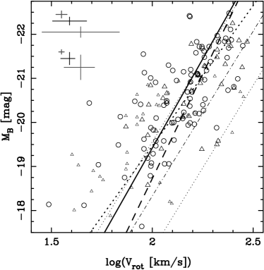
Figure 10: A comparison of our TFR with that of B04. The circular points and solid line are the same is in Fig. 5, as are the thin lines indicating the fiducial PT92 TFR. In addition the ‘high quality’ and ‘low quality’ points from B04 are marked by large and small triangles respectively. The dashed line is a fit to the ‘high quality’ points, and the dotted line is a fit to the full B04 sample. Both of these fits are performed using the same algorithm used to fit our data, as described in Section 3.1. The upper set of error bars in the top left corner indicate the 10th-, 50th- and 90th-percentile uncertainties on the B04 ‘high quality’ points, while the lower set give the same for our full TFR data set.

4 SFR evolution with redshift

We can consider what our best-fitting evolution in the TFR implies for the luminosity and star-formation evolution of field spirals. The implicit assumption in this section is that the $B$-band luminosity of a spiral galaxies with a given rotation velocity evolves due to its star formation history only. For simplicity, we shall parameterise the luminosity and star-formation rate evolution as simple power-laws.

Let us assume that the rest-frame $B$-band luminosity of field spirals evolves as a power law in $(1+z)$. Then,

$$L_{B}(z)=L_{B}(0)\cdot(1+z)^{\beta}$$ (13)

$$\Rightarrow\Delta M_{B}(z)\equiv M_{B}(z)-M_{B}(0)=-2.5\beta\log(1+z)$$ (14)

In Section 3.2 we find a best-fitting evolution with slope

$$\Delta M_{B}(z)\approx(-1.0\pm 0.5)\cdot z\ \mathrm{mag}\;,$$ (15)

which implies $\beta_{\mathrm{fit}}=1.3\pm 0.6$. Fitting directly with respect to $\log(1+z)$ gives the same value for $\beta$.

Before we proceed to compare with stellar evolution models, we need a way to relate $(1+z)$ to time. For the concordance cosmology,

$$(1+z)\approx\left(\frac{t}{t_{0}}\right)^{-0.813}$$ (16)

is an excellent approximation for $z<1$ and sufficiently accurate for our purposes up to $z\sim 5$. For a galaxy of age $t_{\mathrm{age}}$, which formed at $t_{\mathrm{f}}$ we thus have

$$(1+z)\approx\left(\frac{t_{\mathrm{f}}+t_{\mathrm{age}}}{t_{0}}\right)^{-0.813}$$ (17)

Using Eqn. 17 to convert $(1+z)$ to $t_{\mathrm{age}}$ for various $t_{\mathrm{f}}$ we can determine the expected value of $\beta$ for any star-formation history using the stellar evolution models of Bruzual & Charlot (2003). We model the SFR as

$$SFR\propto\left\{\begin{array}[]{ll}0&z>z_{\mathrm{f}}\\ (1+z)^{\alpha}\approx\left(\frac{t_{\mathrm{f}}+t_{\mathrm{age}}}{t_{0}}\right)^{-0.813\alpha}&z\leq z_{\mathrm{f}}\;.\end{array}\right.$$ (18)

For a galaxy with constant SFR ($\alpha=0$) and $z_{\mathrm{f}}=2$ we find $\beta_{\alpha=0}=-0.27$. This corresponds to a brightening of $0.2$ mag between $z=1$ and today. A galaxy with constant SFR is therefore fainter in the past, opposite to what we measure. We therefore require a model with a SFR which declines with time, i.e., $\alpha>0$

The difference in the power-law index between our best-fitting evolution and the constant SFR models is

$$\Delta\beta_{\alpha=0}\equiv\beta_{\mathrm{fit}}-\beta_{\alpha=0}=1.6\pm 0.6\;.$$ (19)

Choosing $z_{\mathrm{f}}=5$ only decreases this slightly to $\Delta\beta_{\alpha=0}=1.5\pm 0.6$. We therefore work with $z_{\mathrm{f}}=2$ hereafter.

In order to have some idea of of what value of $\alpha$ corresponds to what is observed, we can assume that $B$-band luminosity is proportional to the current SFR,

$$\frac{L_{B}}{L_{B,\alpha=0}}=\frac{SFR}{SFR_{\alpha=0}}$$ (20)

which implies $\alpha=\Delta\beta_{\alpha=0}=1.6\pm 0.6$. Putting this form of for the SFR (i.e., SFR $\propto(1+z)^{1.6}$) into the Bruzual & Charlot (2003) code gives

$$\beta_{\alpha=1.6}=1.2\ \Rightarrow\ \Delta\beta_{\alpha=1.6}=0.1\;,$$ (21)

nearly but not quite zero, as Eqn. 20 is not a perfect approximation. However, we can improve our estimate by a straightforward parameter search to determine the value of $\alpha$ which produces our observed $\beta_{\mathrm{fit}}$. We thus find $\alpha=1.7\pm 1.1$.

In summary, we find that SFR$(z)\propto(1+z)^{1.7\pm 1.1}$ in our sample of relatively bright ($M_{B}\ga M^{\ast}_{B}$) galaxies. As we argued earlier, the luminosity evolution determined from our TFR evolution is likely to be an overestimate. The corresponding SFR evolution is therefore probably also an upper limit, and the evolution of the average SFR in luminous spirals may be slower than that found here. In contrast, studies of the SFR density of the Universe at low redshift (e.g., Gallego et al., 1995) and as a function of look-back time (see, e.g., Heavens et al. 2004 for a recent summary) generally indicate a very strong evolution up to $z\sim 1$. The precise rate of this evolution is somewhat controversial, but most studies agree that, parameterizing as SFR $\propto(1+z)^{\alpha}$, $\alpha\simeq 3$–$4$ (see Hopkins 2004 for a compilation of SFR density evolution measurements).

This disparity suggests that the rapid evolution in the SFR density of the universe, observed since $z\sim 1$, is not driven by the evolution of the SFR in individual bright spiral galaxies, like those in our sample. However, it should be noted that, given the size of our sample and the intrinsic scatter in the TFR, the derived constraints on the evolution of SFR in the bright spiral galaxy population are relatively weak. Nevertheless, this kind of approach seems very promising for future studies with samples of several hundred or even thousands of galaxies to $z\sim 1$.

5 Conclusions

We have measured confident rotation velocities for $89$ field spirals with $0.1\la z\la 1$, and used these to examine the evolution of the TFR for these galaxies. The best-fitting TFR for the full sample has a slope which is entirely consistent with that found locally by PT92. There is an intercept offset of $\sim\!1$ mag, such that our galaxies are brighter for a given $V_{\mathrm{rot}}$, but it is likely that this is a least partly due to the differing methods employed to measure the magnitudes and rotation velocities. We therefore only evaluate evolution in the TFR by making internal comparisons of our data.

Fitting sub-samples binned by redshift indicates that the TFR intercept evolves by $\sim\!1$ mag between $z=1$ and today, in the sense that more distant galaxies are brighter for a given $V_{\mathrm{rot}}$. Plotting the residuals of our data from the local TFR against redshift confirms this trend in TFR intercept – higher-redshift galaxies are offset to brighter magnitudes. Fitting this correlation we find an evolution of $-1.0\pm 0.5$ mag by $z=1$, which we argue is an upper limit due to the selection effects present in our sample.

We find no significant evidence for a change in TFR slope. Previous studies have used an observed correlation between the TFR residuals and $V_{\mathrm{rot}}$ to argue that low mass galaxies have evolved significantly more than those with higher mass. However, we have demonstrated that such a correlation may be due solely to an intrinsic coupling between $V_{\mathrm{rot}}$ scatter and TFR residuals, and thus does not necessarily indicate a physical difference in the evolution of galaxies with different $V_{\mathrm{rot}}$.

Finally, we have used the stellar population models of Bruzual & Charlot (2003) to interpret our observed TFR luminosity evolution in terms of a star-formation rate evolution. If the SFR in spiral galaxies had remained constant since $z\sim 1$, their $B$-band luminosity should have increased with time. However, we find the opposite trend, indicating that the SFR in these galaxies was larger in the past. We estimate SFR$(z)\propto(1+z)^{1.7\pm 1.1}$ for our sample. We argue that, given the likely selection effects, this is an upper limit on the SFR increase with look-back time. Our results therefore suggest that the rapid evolution in the SFR density of the universe observed since $z\sim 1$ is not driven by evolution of the SFR in individual bright spiral galaxies.

Even though we cannot yet place strong constraints on the evolution of the SFR in the bright spiral galaxy population, due to our relatively small sample and the intrinsic scatter in the TFR, our approach could be successfully applied in ongoing and future surveys. A study with similar quality data for a sample of $\sim\!600$ galaxies would be needed to reduce the error in $\alpha$ to $\pm 0.4$, providing a clear ($\sim\!3\sigma$) rejection of the hypothesis that the SFR density of the universe and the SFR of the average spiral galaxy evolve at the same rate.

References

- Aragón-Salamanca et al. (1993) Aragón-Salamanca A., Ellis R. S., Couch W. J., Carter D., 1993, MNRAS, 262, 764
- Böhm et al. (2004) Böhm A., et al., 2004, A&A, 420, 97 [B04]
- Bamford et al. (2005) Bamford S. P., Milvang-Jensen B., Aragón-Salamanca A. & Simard L., 2005, MNRAS, 361, 109 [Paper I]
- Barden et al. (2003) Barden M., Lehnert M. D., Tacconi L., Genzel R., White S., Franceschini A., 2003, preprint (astro-ph/0302392)
- Bertin & Arnouts (1996) Bertin E., Arnouts S., 1996, A&AS, 117, 393
- Blanton et al. (2003) Blanton M. R., et al., 2003, ApJ, 592, 819
- Bruzual & Charlot (2003) Bruzual G., Charlot S., 2003, MNRAS, 344, 1000
- Cole et al. (2000) Cole S., Lacey C. G., Baugh C. M., Frenk C. S., 2000, MNRAS, 319, 168
- Couch & Sharples (1987) Couch W. J., Sharples R. M., 1987, MNRAS, 229, 423
- Couch et al. (1998) Couch W. J., Barger A. J., Smail I., Ellis R. S., Sharples R. M., 1998, ApJ, 497, 188
- Dale et al. (1997) Dalcanton J. J., Spergel D. N., Summers F. J., 1997, ApJ, 482, 659
- Dale et al. (1999) Dale D. A., Giovanelli R., Haynes M. P., Campusano L. E., Hardy E., 1999, AJ, 118, 1489
- Dressler et al. (1999) Dressler A., Smail I., Poggianti B. M., Butcher H., Couch W. J., Ellis R. S., Oemler A. J., 1999, ApJS, 122, 51
- Ferreras et al. (2004) Ferreras I., Silk J., Böhm A., Ziegler B., 2004, MNRAS, in press
- Gallego et al. (1995) Gallego J., Zamorano J., Aragón-Salamanca A., Rego M., 1995, ApJ, 455, L1
- Gioia et al. (1998) Gioia I. M., Shaya E. J., Le Fevre O., Falco E. E., Luppino G. A., Hammer F., 1998, ApJ, 497, 573
- Heavens et al. (2004) Heavens A., Panter B., Jimenez R., Dunlop J., 2004, Nature, 428, 625
- Hopkins (2004) Hopkins, A. M., ApJ. 615, 209
- Koda et al. (2000) Koda J., Sofue Y., Wada K., 2000, ApJ, 531, L17
- Loveday (2004) Loveday J., 2004, MNRAS, 347, 601
- Milvang-Jensen (2003) Milvang-Jensen B., 2003, PhD thesis, University of Nottingham
- Milvang-Jensen et al. (2003) Milvang-Jensen B., Aragón-Salamanca A., Hau G. K. T., Jørgensen I., Hjorth J., 2003, MNRAS, 339, L1
- Norberg et al. (2002) Norberg P., et al., 2002, MNRAS, 336, 907
- Persic & Salucci (1991) Persic M., Salucci P., 1991, ApJ, 368, 60
- Pierce (1994) Pierce M. J., 1994, ApJ, 430, 53 [P94]
- Pierce & Tully (1992) Pierce M. J., Tully R. B., 1992, ApJ, 387, 47 [PT92]
- Rix et al. (1997) Rix H.-W., Guhathakurta P., Colless M., Ing K., 1997, MNRAS, 285, 779
- Schechter (1976) Schechter, P. 1976, ApJ, 203, 297
- Schlegel et al. (1998) Schlegel D. J., Finkbeiner D. P., Davis M., 1998, ApJ, 500, 525
- Seifert et al. (2000) Seifert W., et al., 2000, in Masanori I., Moorwood A. F., eds, Proc. SPIE Vol. 4008, Optical and IR Telescope Instrumentation and Detectors, p. 96
- Silk (1997) Silk J., 1997, ApJ, 481, 703
- Simard & Pritchet (1998) Simard L., Pritchet C. J., 1998, ApJ, 505, 96
- Simard & Pritchet (1999) Simard L., Pritchet C. J., 1999, PASP, 111, 453
- Simard et al. (1999) Simard L., et al., 1999, ApJ, 519, 563
- Simard et al. (2002) Simard L., et al., 2002, ApJS, 142, 1
- Smail et al. (1997) Smail I., Dressler A., Couch W. J., Ellis R. S., Oemler A. J., Butcher H., Sharples R. M., 1997, ApJS, 110, 213
- Spergel et al. (2003) Spergel D. N., et al., 2003, ApJS, 148, 175
- Tully & Fisher (1977) Tully R. B., Fisher J. R., 1977, A&A 54, 661
- Tully & Fouque (1985) Tully R. B., Fouque P., 1985, ApJS, 58, 67
- Tully & Pierce (2000) Tully R. B., Pierce M. J., 2000, ApJ, 533, 744
- Tully et al. (1998) Tully R. B., Pierce M. J., Huang J., Saunders W., Verheijen M. A. W., Witchalls P. L., 1998, AJ, 115, 2264
- van Dokkum et al. (2000) van Dokkum P. G., Franx M., Fabricant D., Illingworth G. D., Kelson D. D., 2000, ApJ, 541, 95
- Verheijen (2001) Verheijen M. A. W., 2001, ApJ, 563, 694
- Vogt et al. (1996) Vogt N. P., Forbes D. A., Phillips A. C., Gronwall C., Faber S. M., Illingworth G. D., Koo D. C., 1996, ApJ, 465, L15
- Vogt et al. (1997) Vogt N. P., et al., 1997, ApJ, 479, L121
- Vogt et al. (2002) Vogt N. P., et al., 2002, Bulletin of the American Astronomical Society, 34, 703
- Willick (1994) Willick J. A., 1994, ApJS, 92, 1