New evolutionary calculations for the Born Again scenario

We present evolutionary calculations aimed at describing the born-again scenario for post-AGB remnant stars of 0.5842 and 0.5885 M_⊙. Results are based on a detailed treatment of the physical processes responsible for the chemical abundance changes. We considered two theories of convection: the standard mixing length theory (MLT) and the double-diffusive GNA convection developed by Grossman et al. The latter accounts for the effect of the chemical gradient ($\nabla\mu$) in the mixing processes and in the transport of energy. We also explore the dependence of the born-again evolution on some physical hypothesis, such as the effect of the existence of non-zero chemical gradients, the prescription for the velocity of the convective elements and the size of the overshooting zones. Attention is given to the behavior of the born-again times and to the chemical evolution during the ingestion of protons. We find that in our calculations born again times are dependent on time resolution. In particular when the minimum allowed time step is below $5\times 10^{-5}$ yr we obtain, with the standard mixing length theory, born again times of 5-10 yr. This is true without altering the prescription for the efficiency of convective mixing during the proton ingestion. On the other hand we find that the inclusion of the chemical gradients in the calculation of the mixing velocity tend to increase the born again times by about a factor of two. In addition we find that proton ingestion can be seriously altered if the occurrence of overshooting is modified by the $\nabla\mu$-barrier at the H-He interface, strongly altering born again times.

1 Introduction

The surface chemical composition that characterizes post-asymptotic giang branch (AGB) stars is diverse and poses a real challenge to the stellar evolution theory. In particular, about 20% of these objects exhibit hydrogen(H)-deficient surface compositions. The most widely accepted mechanism for the formation of H-deficient stars remains the born again scenario, which develops as a result of a last helium thermal pulse that occurs after the star has left the thermally pulsing AGB. If this pulse happens when H-burning has almost ceased on the early white-dwarf cooling branch, it is classified as a very late thermal pulse (VLTP). In a VLTP, the outward-growing convection zone powered by helium burning reaches the base of the H-rich envelope. As a result, most of H is transported downwards to the hot helium burning region, where it is completely burned.

Observational examples of stars that are believed to have experienced a born-again episode are the oxygen-rich, H-deficient PG-1159 stars and the Wolf Rayet type central stars of planetary nebulae having spectral type [WC] (Dreizler & Heber 1998 and Werner 2001). In particular, the high surface oxygen abundance detected in these stars has been successfully explained in terms of overshoot episodes below the helium-flash convection zone during the thermally pulsing AGB phase (Herwig et al. 1999, see also Althaus et al 2005).

Both theoretical and observational evidence (Dreizler & Werner 1996, Unglaub & Bues 2000 and Althaus et al. 2005) suggest an evolutionary connection between most of PG1159 stars and the helium-rich DO stars, the hot and immediate progenitors of the majority of DB white dwarfs. Thus, the born again process turns out to be a key phenomenon in explaining the existence of the majority of DB white dwarfs. In addition, the identification of the Sakurai’s object (V4334 Sgr) as a star just emerging from a born-again episode (Duerbeck & Benetti 1996) has led to a renewed interest in assessing the evolutionary stages corresponding to the VLTP and the ensuing born-again. V4334 Sgr has been observed to suffer from an extremely fast evolution. Indeed, it has evolved from the pre-white dwarf stage into a giant star in only about a few years (see Asplund et al. 1999, Duerbeck et al. 2000). Also recent observations (Hajduk et al. 2005) seem to indicate that Sakurai’s object is quickly reheating. Unfortunately, very few detailed numerical simulations through the born-again stage regime exist in the literature. Evolutionary calculations that incorporate appropriate time-dependent mixing procedures were carried out initially by Iben & MacDonald (1995), who found short born-again time scales of about 17 yr. By contrast, Herwig et al.(1999) and Lawlor & MacDonald (2003) derived too large born-again timescales, typically 350 yr, to be consistent with observations. This has prompted Herwig (2001) to suggest that, in order to reproduce the observed born again timescale, the convective mixing velocity ($v_{\rm MLT}$) in the helium burning shell should be substantially smaller than that given by the standard mixing length theory of convection (MLT). In fact, Herwig (2001) finds that a reduction in the MLT mixing diffusion coefficient $D$ ($D=\frac{1}{3}\,\alpha_{\rm MLT}\,v_{\rm MLT}$) by a factor 100 is required to arrive at an agreement with observations (see also Lawlor & MacDonald 2003 and Herwig 2002 for a similar conclusion). The reason for the discrepancy between the theoretical born again time scales is not clear.

In this paper we present new detailed evolutionary calculations for the born-again phase by using an independent stellar code that allows us to follow in detail the abundance changes that take place throughout all the VLTP phase. Specifically, we analyze the VLTP evolution of 0.5842 and 0.5885 M_⊙ remnant stars, the previous evolution of which has been carefully followed from initially 2.5 and 2.7 $M_{\odot}$ ZAMS star models to the thermally pulsing AGB stage and following mass loss episodes. The value of the stellar mass of our post-AGB remnant allows us to compare our predictions with the observations of the Sakurai’s object characterized by a stellar mass value between 0.535 and 0.7 $M_{\odot}$ (Herwig 2001). We examine the dependence of our evolutionary time scales and the phase of proton ingestion on some numerical and physical parameters. We extend the scope of the paper by exploring the role played by the molecular weight gradient ($\nabla\mu$) induced by proton burning by considering the double-diffusive MLT for fluids with composition gradients (Grossman & Taam 1996). To the best of our knowledge, this is the first time that this effect is incorporated in the calculation of a VLTP. The following section describes the main physical inputs of the evolutionary models, in particular the treatment of the chemical abundance changes in the convective regions of the star. Also a brief description of the evolution of the stars prior to the VLTP is given. In addition, we analyze how the physical hypotheses made in the modeling of the star set restrictions on the possible time-resolution during the VLTP, and then the effects of a bad time-resolution during the proton burning are described. In Sect. 3, we present our results, particularly regarding the born-again evolutionary time scales and proton burning.In Sect. 4 we explore the dependence of the born again time scale on numerical and physical details. In Sect. 5 we provide a comparison with observations. And finally, in Sect. 6 we close the paper by making some concluding remarks.

2 Input physics and numerical details

2.1 The stellar evolution code

The evolutionary calculations presented in this work have been carried out with the stellar evolution code LPCODE. A detailed description of the code, both in its numerical aspects as well as in its input physics, has been given in Althaus et al. (2003) and references therein.

Here, we only briefly review the treatment given to the chemical abundance changes, a key point in the computation of the short-lived VLTP phase and the ensuing born-again evolution. Indeed, such phases of evolution are extremely fast to such an extent that the time-scale of the nuclear reactions driving the evolution of the star becomes comparable to the convective mixing timescale. Accordingly, the instantaneous mixing approach usually assumed in stellar evolution breaks down and, instead, a more realistic treatment which consistently couples nuclear evolution with time-dependent mixing processes is required. Specifically, the abundance changes for all chemical elements are described by the set of equations

$$\left(\frac{d\@vec{Y}}{dt}\right)=\left(\frac{\partial\@vec{Y}}{\partial t}\right)_{\rm nuc}+\frac{\partial}{\partial M_{r}}\left[\left(4\pi r^{2}\rho\right)^{2}D\frac{\partial\@vec{Y}}{\partial M_{r}}\right],$$ (1)

with $\@vec{Y}$ being the vector containing the mole fraction of all considered nuclear species. Mixing is treated as a diffusion process which is described by the second term of Eq. (1) for a given appropriate diffusion coefficient (see below). The first term in Eq. (1) gives the abundance changes due to thermonuclear reactions. Changes both from nuclear burning and mixing are solved simultaneously and numerical details can be found in Althaus et al. (2003). The present version of LPCODE accounts for the evolution of 16 isotopes and the chemical changes are computed after the convergence of each stellar model. A more accurate integration of the chemical changes is achieved by dividing each evolutionary time step into several chemical time steps.

The treatment of convection deserves some attention because not only does it determine how heat is transported in non-radiative regions, but also because it determines the efficiency of the different mixing process that can occur in the star. In the present investigation, we have considered two different local theories of convection. On one hand, the traditional Mixing Length Theory (MLT) assuming that the boundaries of the convective regions are given by the Schwarzschild criterion. In this case, mixing is restricted only to convective unstable regions (and the adyacent overshooting layers, as mentioned below). On the other hand, we have also considered the double diffusive mixing length theory of convection for fluids with composition gradients developed by Grossman et al. (1993) in its local approximation as given by Grossman & Taam (1996) (hereafter GT96). The advantage of this formulation is that it applies consistently to convective, semiconvective and salt finger instability regimes. In particular, it accounts for the presence of a non-null molecular weight gradient $\nabla\mu$. This will allow us to explore the consequences of the chemical inhomogeneities that develop in the convection zone resulting from the fast ingestion of protons during the born-again evolution. As mentioned, the GNA theory describes mixing episodes not only at dynamically unstable regions (Schwarzschild-Ledoux criterion), but also accounts for “saltfinger” and “semiconvective” regimes. Both of these regimes are consequence of a non zero thermal diffusion rate. In particular saltfinger mixing takes place in those layers with negative chemical gradient ($\nabla\mu<0$, i.e. heavier elements are above lighter ones) and it is a process far less efficient than the ordinary convective instability (dynamical instability).

Overshooting has been adopted by following the formulation of Herwig et al. (1997) and applied to all convective boundaries in all our evolutionary calculations. The adopted overshooting parameter $f$ is 0.016 unless otherwise stated, because this value accounts for the observed width of the main sequence and abundances in H-deficient, post-AGB objects (Herwig et al. 1997, Herwig et al. 1999, Althaus et al. 2005). It should be noted, however, that there is no physical basis so far supporting a unique choice of $f$ for so different situations in which convection is present in stars.

Before presenting our evolutionary calculations, let us discuss a few numerical issues. Their importance will be made clearer in Sect. 4, where results are presented.

2.2 Time Resolution during the ingestion of protons

Evolution during the VLTP is characterized by extremely fast changes in the structure of the star. This is particularly true regarding the development of the H burning flash when protons from the stellar envelope are mixed into the hot helium-burning shell. As was noted by Herwig (2001) the minimum time step (MTS) used during the proton burning has to be kept consistent with the hypotheses made in the modeling of the star. In particular this means that the MTS must remain larger than the hydrodynamical time scale, that is of the order of

$$\tau_{\rm hydr}\sim\sqrt{\frac{R^{3}}{GM}}.$$ (2)

At the onset of the VLTP and during the ingestion of protons ($R=2.36\times 10^{9}$cm) $\tau_{\rm hydr}$ is about 12.9s. In addition, we have checked that the hydrostatic approximation is fulfilled to a high degree, as

$$\frac{1}{4\pi r^{2}}\frac{\partial^{2}r}{\partial t^{2}}\mathrel{\hbox{\hbox to0.0pt{\hbox{\lower 4.0pt\hbox{$\sim$}}\hss}\hbox{$<$}}}10^{-4}\frac{Gm}{4\pi r^{4}}.$$ (3)

in every mesh point during the H flash and the first years after it. Also, the MTS has to be kept larger than the convective turn-over time (i.e. the time for the temperature gradient to reach the values predicted by the mixing length theory, or any other time-independent convection theory). This time scale can be estimated as the inverse of the Brünt-Väisälä frequency, which yields the time it takes a bubble to change its temperature in a convectively unstable zone (Hansen & Kawaler 1994), that is

$$\tau_{\rm conv}\sim\frac{1}{|N|}=\sqrt{\frac{kT}{\mu m_{H}g^{2}|\nabla-\nabla_{\rm ad}|}}.$$ (4)

At the conditions of proton burning during the VLTP ( $T\sim 10^{8}K$, $g\sim 1.5\times 10^{7}cm/s^{2}$ and $(\nabla-\nabla_{\rm ad})\sim 10^{-3}$), $\tau_{\rm conv}\sim 4.6$ minutes. This value depends somewhat on the exact position of the proton burning zone, but it is always of only a few minutes.

In order to be consitent with the assumed hypotheses we should use MTS greater than $10^{-5}$yr (i.e. greater than 5 minutes). This could be problematic if the results for the born again time-scale would present a dependence on the election of MTS during the proton burning phase, (to be described in the following section) even for smaller values of the MTS. Fortunately, as will be clear later, all our theoretical sequences computed with ${\rm MTS}<5\times 10^{-5}$yr yield born-again time-scales that are, for practical purposes, independent of the MTS value, while being consistent with the fundamental hypothesis.

2.3 Errors due to bad time-resolution during the peak of proton burning

We have computed various VLTP sequences with different time resolutions (i.e. by setting different values of MTS) during the vigorous proton burning episode. In order to get an error estimation in the evaluation of $L_{\rm H}$, the proton-burning luminosity (Herwig 2001 and also Schlattl et al. 2001), we have calculated its value at each time step from the H mass burned in that time interval (let us denote it $L{\rm{}^{X}_{H}}$), and compared it to the value integrated in the structure equations ($L{\rm{}^{S}_{H}}$).

Chemical changes are followed with a smaller time step than the one used for the structure equations (typically 3-5 times smaller). As a result, $L{\rm{}^{X}_{H}}$ would be expected to be closer to the actual value of proton-burning luminosity than $L{\rm{}^{S}_{H}}$. However, it should be noted that due to the fact that the chemical changes are calculated using a fixed stellar structure, during the onset of H burning, when the outer border of the convective zone penetrates into more H-rich layers, the value of $L{\rm{}^{X}_{H}}$ will be lower than it should be if the advance of the convective zone $during$ the calculation of the chemical changes were taken into account . Thus, the actual value of $L_{H}$ may be, for small MTS, slightly greater than that estimated from $L{\rm{}^{X}_{H}}$ (see Schlattl et al. 2001 for a similar consideration).

Figure 1: Estimation of the errors involved in $L_{H}$ (for different MTS) during the peak of proton burning for the different models calculated with the MLT. Thick lines correspond to models previous to the maximum of proton burning, while thin lines show the errors after the maximum of $L_{H}$

We find that for MTS smaller than $5\times 10^{-5}$yr ($3\times 10^{-5}$,$10^{-5}$ and $3\times 10^{-6}$yr) the porcentual error in $L_{H}$ is always below $10\%$ during the onset of proton burning. Note that by using a MTS of $1\times 10^{-5}$yr the error is kept lower than $3\%$ during the onset of proton burning. On the other hand, when we use values of MTS greater than $10^{-4}$yr the error grows to $50\%$ and even up to $100\%$ for an MTS of $10^{-3}$yr. In Fig. 1 the estimated error of $L_{\rm H}$ during proton burning is shown for sequences with different MTS values.

As it will be shown in Sect. 3.2.1, the value of $L{\rm{}_{H}}$ and the size of the convective zone powered by proton burning (proton-burning convection zone, PBCZ) are expected to be closely related because an increase in the energy flux tends to promote instability against convection even further out in the H-rich envelope, while an increase in the PBCZ extension into the H-rich envelope will increase the value of $L_{H}$ as more protons will become available for being burned at the bottom of the convection zone (Iben et al. 1983, Schlattl et al.2001). Thus, we expect this process to be particularly sensitive to errors in the value of $L{\rm{}^{S}_{H}}$ at each time step.

Figure 2: Evolutionary track for the complete evolution of an initially 2.5 M_⊙ star model from the ZAMS through the AGB, a very late thermal pulse (VLTP) to the start of the cooling branch as a 0.5842 M_⊙ hot white dwarf. Note the occurrence of the VLTP at high effective temperature when the post-AGB remnant has almost reached the cooling branch. Relevant episodes during and after the VLTP are pointed out.

3 Evolutionary results

3.1 Prior evolution

For consistency purposes, the initial VLTP stellar configurations employed in this study are the result of the complete evolution of progenitor stars, starting originally from the ZAMS and going through the thermally pulsing AGB phase. Unfortunately, the considerable amount of computing time demanded by our self-consistent solution of nuclear evolution and time-dependent mixing, has restricted ourserlves to examining only two cases for the complete evolution for the progenitor star. Specifically, the evolution of an initially 2.5 M_⊙ stellar model was computed from the zero-age main sequence all the way from the stages of H and helium burning in the core up to the tip of the AGB where helium thermal pulses occur. In addition we compute the full evolution of an initially 2.7 M_⊙ stellar model (see Althaus et al. 2005 for details) which experiences a VLTP somewhat earlier than the 2.5 M_⊙ sequence. The stellar masses of the post AGB remnants are 0.5842 and 0.5885 M_⊙ for the 2.5 and 2.7 M_⊙ respectively. A total of 10 and 12 thermal pulses on the AGB have been calculated. At the moment of the born again the total H-mass of the models is $8.5\times 10^{-5}$ and $6.3\times 10^{-5}$ M_⊙.

For both sequences overshoot episodes taking place during central burning stages as well as during the thermally pulsing AGB phase have been considered. A solar-like initial composition $(Y,Z)=(0.275,0.02)$ has been adopted. The complete Hertzsprung-Russell diagram for the 2.5 $M_{\sun}$ sequence is illustrated in Fig.2. The evolutionary stages for the progenitor star (on the cool side of effective temperatures) starting from the ZAMS as well as the VLTP-induced born again episode and the post born again evolution towards the white dwarf regime are clearly visible. Relevant episodes during the VLTP and the ingestion of protons are indicated as well. As a result of mass losses the stellar mass is reduced to 0.5842 M_⊙. After the born again episode and before the domain of the central stars of planetary nebulae at high effective temperatures is reached, the now H-deficient remnant evolves through a double loop path. Mass loss episodes during and after the VLTP were not considered.

3.2 Evolution through the VLTP

In the rest of this section, we restrict the presentation of evolutionary results to the 2.5 M_⊙ (0.5842 M_⊙ remnant) sequence, computed with MTS= $1\times 10^{-5}$yr and with the MLT.

3.2.1 Evolution during the ingestion of protons

Figure 3: Evolution of the outer convective border of the PBCZ and the inner chemical abundances as a function of mass coordinate during the ingestion of protons through the VLTP. Grey bars denote convective regions, and dotted bars mark overshoot regions. Panel A shows the interior abundances at the moment the He-driven convective zone reaches the region where H has been partially burned through CNO reactions before the VLTP. Panel B displays the interior compositions at the moment of the splitting of the convective region, when convection has reached layers with $X\sim 0.08$. Finally, panel C corresponds to the moment of maximum H-burning energy release.

During the VLTP, the convection zone powered by the helium shell burning grows in mass until its outer edge reaches the H-rich envelope, at variance with the situation encountered in AGB models where the presence of a high entropy barrier due to H burning prevents this from occurring. This is shown in panel A in Fig. 3. It must be noted that the composition at the base of the H envelope is not homogenous because it is the result of previous H burning (keep in mind that stars experiencing a VLTP must have left the AGB during the phase of H-shell burning). As this shell (whose width is of 0.00015 ${\rm M_{\odot}}$) has a H abundance with a marked depth dependence (see Fig. 3), proton burning rises as layers with a larger amount of H are reached by convection. When the outer border of the convection zone reaches layers where $X_{H}\sim 0.035$, $\log{\left(L{\rm{}_{H}/L_{\odot}}\right)}$ becomes as high as 3. About 2.8 days later, the convective shell has reached regions with $X_{H}\sim 0.08$ and $\log{\left(L{\rm{}_{H}/L_{\odot}}\right)}$ has risen to $\sim 6.5$ (panel B). Temporal evolution of $L_{\rm H}$ can be followed in Fig. 4, where also models corresponding to A, B and C panels of Fig. 3 are marked in the upper inset. At this point, two important things take place. First, as a consequence of the large amount of energy generated in the H burning shell, the original convective region splits into two distinct convective zones connected by an overshooting intershell region (see lower inset of Fig. 4). The upper convection zone is the proton-burning convection zone (PBCZ), while the lower one is powered by helium burning. Second, a sudden outwards excursion of the PBCZ causes an enhanced transport of material from the unprocessed H-rich envelope downwards to hotter layers where protons are vigorously burnt, with the consequence that the PBCZ is pushed even further out. This second stage of proton burning is extremely violent and short-lived. In fact, in only 15.4 hours $\log{\left(L{\rm{}_{H}/L_{\odot}}\right)}$ increases from 6.5 to more than 11. The sudden increase in the convective region can be seen by comparing the location of the outer border of the PBCZ in panels B and C of Fig. 3, where the last one corresponds to the maximum in $L_{H}$, as shown in Fig. 4. According to this description proton burning during the VLTP can be separated into two stages (a similar situation has been reported by Schlattl et al. 2001 during the ingestion of protons in the core He flash of low metallicity stars) The first one lasts for about 25 days while $\log{\left(L{\rm{}_{H}/L_{\odot}}\right)}\mathrel{\hbox{\hbox to0.0pt{\hbox{\lower 4.0pt\hbox{$\sim$}}\hss}\hbox{$<$}}}6.5$ and the outer convective border is pushed forward mostly by He-burning. The second stage occurs when the energy liberated by H-burning becomes comparable to the He-burning energy release, the convective zone splits into two and the newly formed PBCZ is pushed outwards by proton burning (and lasts for only a few hours). As will be shown in Table 1, this feedback between the increase in the size of the PBCZ and the value of $L_{H}$ is expected to make that moderate initial errors in the calculation of $L_{H}$ will enhance and produce very different integrated values of $L_{H}$ during the born-again evolution, yielding different maximum values for $L_{H}$ as well. Indeed, it is this stage of proton burning which is seriously altered when we use large MTS, see discussion in Sect. 4.

Finally, let us say that the violent proton burning occurs initially mainly through the chain ¹²C$+p\rightarrow^{13}{\rm N}+\gamma\rightarrow^{13}{\rm C}+e^{+}+\nu_{e}$ due to the extremely high ${}^{12}{\rm C}$ abundance in the He-shell. This changes as more ${}^{12}{\rm C}$ is processed into ${}^{13}{\rm C}$ and the reaction ${}^{13}{\rm C}+p\rightarrow^{14}{\rm N}+\gamma$ becomes more important. At the end of the ingestion of protons both reactions are generating energy at comparable rates.

Figure 4: Evolution of $L_{\rm H}$ during the born-again phase (black dots in the upper inset mark the position of panels A, B, and C in Fig. 3). The lower inset shows the diffusion coefficient ($\log{D}$ in cm²s^-1) and the energy release ($\log{\epsilon}$ in erg g^-1 s^-1), at the moment just before (continuous lines) and after (broken lines) the splitting of the original convective region (which causes the drop in $D$ at M/M_⊙$\sim$ 0.577) into a He-burning-driven convective zone and an overlying H-burning-driven convective zone.

Figure 5: Evolution of the surface temperature for the sequence described in section 3 (continuous lines). The zero point of the x-axis of the observations has been arbitrarily fixed in order to allow for comparison with the theoretical cooling rate. Triangles mark the data derived by Duerbeck et al. (1997) (empty triangles correspond to less reliable data), while crosses correspond to Asplund et al. (1999). Note the short born again timescale (about 5 years) displayed by the model. Also the evolution of the effective temperature for a model which suffers from an “early” VLTP (section 4.1, dash dotted line) and for a model with a slight reduction of the mixing efficiency ($D$/3, section 4.5, dotted line) are shown. Inset shows the evolution of the lightcurves for the previous models.

3.3 Further Evolution

After the occurrence of the He-flash and the subsequent violent proton burning the model expands and returns to the giant region of the HR diagram in only about 5 yr, which is of the order of the observed timescale of the Sakurai’s object and V605 Aql. Fig. 5 shows the evolution of $T_{\rm eff}$. It is important to note here that the short evolutionary time-scales are obtained without invoking a reduction in the mixing efficiency, as claimed necessary in some previous works (Herwig 2001 and Lawlor & MacDonald 2003). The star remains in the red giant domain without changing its effective temperature significantly ( log$T_{\rm eff}\mathrel{\hbox{\hbox to0.0pt{\hbox{\lower 4.0pt\hbox{$\sim$}}\hss}\hbox{$<$}}}3.7$) for the next 26 yrs. Although this is at variance with the reported quick reheating of Sakurai’s object (Hajduk 2005), for log$T_{\rm eff}$ below 3.8 we do not expect our models to be a good description of what is really happening. This could be because modeling hypothesis, in particular the hydrostatical approximation, are not fulfilled in the outer shells of the model . During this stage the surface luminosity rises and the layers at the bottom of the convective envelope attain the conditions where the value of the radiation pressure becomes high enough to balance the effect of gravity (Eddington limit, see figure 6). When this happens gas pressure tends to zero, and hydrostatic equilibrium hypothesis is broken there. This causes our calculations to become unstable (see also Lawlor & MacDonald 2003 in one of their sequences). The Eddington limit provides a natural mechanism to separate the envelope from the rest of the star (see Faulkner & Wood 1985). To proceed with the calculations, we artificially force the outermost envelope to be in thermal equilibrium (i.e. $dS/dt=0$), this was done by extending the envelope integration downwards to shells where the Eddington limit was reached (this happened 15 yr after the H flash). We note that by doing this we do not alter the surface abundances of the star (nor its total mass), as the chemical profile has been previously homogeinized by convection throughout the envelope. In the next five years the remnant star increases its surface temperature from $\sim 3.8$ to $\sim 4.35$, and in only 20 $yr$ its temperature increases up to $\sim 4.6$ (Fig. 5). However these times appear to be dependent on the detailed treatment of the outer shell of the envelope. About 100 $yr$ after the H flash the star reaches temperatures above log$T_{\rm eff}=4.8$ and starts the He driven expansion which ends at log$T_{\rm eff}\sim 3.7$ and lasts for about 250 $yr$ (this is 350 $yr$ after the H flash). Finally after reaching the giant region for the second time the remnant contracts again and moves to the PG1159 domain. These comings and goings in $T_{\rm eff}$ caused by H and He-burning driven expansions produce the typical double loop in the HR diagram (see Fig. 6 and also Lawlor & MacDonald 2003 and Herwig 2003).

Figure 6: HR diagram for the evolution after the VLTP. Here we see the typical double loop pattern due to sucesive H and He driven expansions. Also the location where our model reaches the Eddington limit is shown.

4 Born-again time-scales: dependence on numerical and physical details

In this section we discuss a variety of issues, both on numerics and physics, that may affect the computed evolutionary time-scales of born-again episodes. The reader not interested in these details can refer directly to Sect. 5 where discussion of the results and comparison with observations are presented.

As mentioned early in the introduction, theoretical models of the born again phenomena do not agree on the predicted born again times for a $\sim 0.6\rm M_{\odot}$ star. These times range from about $\sim$17 yr in Iben & MacDonald (1995) to 350 yr as in Herwig (1999) and Lawlor & MacDonald (2003). In addition the extremely fast evolution of Sakurai’s object has posed a challenge to stellar evolutionary calculations, which have been unable to reproduce the observed short timescale unless a high reduction in the mixing efficiency (of about a factor of 100-1000, Herwig 2001 and Lawlor & MacDonald 2003) is assumed. On the contrary, our evolutionary calculations are able to reproduce born again times of about 5 yr (closer to the observed ones) $without$ changing the mixing efficiency of the models (see Fig.  5). In fact we are able to reproduce born again times as short as 3 yr by invoking a reduction in the mixing efficiency by only a factor of 3. We note that our stellar masses are somewhat smaller than the 0.604 M_⊙ used in Herwig (2001). Although this mass difference is expected to reduce the born again times (Herwig 2001), it cannot account for the whole difference in the timescales. In this connection note that the low mass model (0.535 M_⊙) presented by Herwig (2001) displays ages still larger than those derived from our models.

In view of the different results obtained by different research groups, we think it is worth investigating how the born-again time-scale depends on different details entering the calculations, i.e. numerics and input physics. In this section we try to address some of these issues.

4.1 Results for an early-VLTP sequence

Figure 7: Same as Fig. 2 but for a model which suffers from an “early” VLTP (this is at luminosities about one order of magnitude larger than in the model shown in Fig. 2).The inset shows the temporal evolution of $L_{H}$ for this model. Note that the evolution is less violent than in the previous case (compare upper inset of Fig. 4) and that the two stages of proton burning are more easily differentiated.

Here we explore the expectations for the 0.5885 M_⊙ model that experiences a VLTP earlier (i.e. at higher luminosities, log$(L/L_{\odot})\sim 3$) than the 2.5 M_⊙ sequence . At the moment of the VLTP the object is less compact and the flash takes place in a less degenerate environment, as compared with the 2.5 M_⊙ sequence. Also note that the total H-mass in the model (which is almost completely burned during the VLTP) is lower in this case. Therefore, the proton ingestion described in section 3.2.1 is less violent. As can be seen in the inset of Fig. 7 the two stages of proton burning are more distinguishable than in the previous case. Longer times are needed for the H-flash to develope. In this case the first stage of proton burning (the one before the splitting of the convective regions, when the outer convective border is driven mainly by He-burning) lasts for about 0.3 yr, while the second more violent stage takes about 2.5 days. Also note that the magnitude of $L_{H}$ at the maximum is lower than in the previous model, reaching a value of log$(L_{H}/L_{\odot})\sim 9.8$. Consequently we find that born again times are longer in this case, taking about 8.7 yr (see Fig. 5 and 8) when a standard MTS of $10^{-5}$ yr is adopted during the H-flash (Table 1).

4.2 Time resolution

In this, and in the following sections, the results correspond to the 2.7 M_⊙ sequence.

MTS	$\int{L{\rm{}_{H}dt}}$ [erg]	$\Delta t$ [days]	Born-again
		$L_{H}>(e^{-1}\times{L_{H}}_{\rm max})$	time-scale [yr]
$1\times 10^{-5}$	$4.5\times 10^{47}$	0.113	8.7
$3\times 10^{-5}$	$4.31\times 10^{47}$	0.133	10.3
$1\times 10^{-4}$	$3.75\times 10^{47}$	0.209	21
$5\times 10^{-4}$	$2.59\times 10^{47}$	0.777	280

Table 1: Characteristic values for the VLTP, for various MTS values. Note the dispersion in born again times according to the adopted MTS value. Third column shows a characteristic time for the duration of the peak of proton burning. The born-again times correspond to the time interval from the moment of maximum $T_{\rm eff}$ after the H burning (and at high luminosity) until $\log{T_{\rm eff}}=3.8$ is reached for the first time.

In Sect. 2.2 we discussed the constraints imposed on the MTS choice by basic assumptions implicit in stellar evolutionary calculations, namely those of hydrostatic equilibrium and the use of time-independent theory of convection. Then in Sect 2.3 it was noted that the chemical integration scheme used in this work was sensitive to the adopted time resolution. Now we analyze how a poor time resolution affects the energy liberation and, consequently, the born again times.

In Table 1 we show some characteristic values of the violent proton burning for different calculations of the process according to the MTS employed. Note from Fig. 1 that a poor time resolution yields $L{\rm{}^{S}_{H}}$ values that are underestimated with respect to $L{\rm{}^{X}_{H}}$ by more than an order of magnitude (for the definition of $L{\rm{}^{S}_{H}}$ and $L{\rm{}^{X}_{H}}$ see Section 2.3). Also note that when evolution is calculated using a MTS of $5\times 10^{-4}$ yr, the energy is liberated over a period $\sim 7$ times larger, and the total energy liberated by proton burning is $40\%$ smaller than in the standard case with MTS $=10^{-5}$yr. As a result the born again timescale strongly depends on the election of the MTS, as shown in Fig. 8 (see also Fig. 9 where the rate of energy generation per unit gram, at the peak of proton burning, changes one order of magnitude) . A large value of the MTS leads to born-again time-scales of the order of 300 yr, which are typical values corresponding to born-again episodes driven by helium-burning (Iben et al., 1983). When time resolution is improved and the MTS is chosen to be lower that $5\times 10^{-5}$ yr much shorter evolutionary times for the born-again event are obtained. As can be seen in Fig. 8, it takes only 10 yr for the remnant to evolve from the white dwarf configuration to giant dimensions. This dependence can be understood in terms of the large errors (between 30% and 100%) that lead to an underestimation of $L{\rm{}^{S}_{H}}$ when large MTS are used; while taking MTS shorter than $5\times 10^{-5}$ yr keeps these errors below the 10% level (Fig. 1 and Table 1). It is interesting to note that these changes in the born-again time-scales are not related with the position of the maximum proton-burning zone in the models, which is the same irrespective of the MTS used, as illustrated in Fig. 9. A final important point to be remarked is the convergence we find for the evolutionary times, i.e. using MTS values smaller than $5\times 10^{-5}$ yr do not lead to shorter timescales. This seems to indicate that errors in the evaluation of $L{\rm{}^{S}_{H}}$ are under control and that results for the time-scales are robust, at least regarding the time-step choice.

Figure 8: Evolution of the surface temperature for models calculated with different MTS. Note the high dependence of the born again times with the chosen time resolution during the H-flash when the MTS is above $5\times 10^{-5}$ yr. In particular note that for a very poor time resolution (MTS$\sim 5\times 10^{-4}$ yr) the H-driven expansion is almost totally suppressed.

Figure 9: Nuclear energy generation due to helium and proton burning as a function of the mass coordinate for various MTS values. The most external peak shown corresponds to the energy released by proton burning. Note the change in the energy release resulting from different time resolution. This is because a good time resolution leads to a more violent proton ingestion, and thus to a higher H-burning rate. Indeed, this caused both a change in the total energy generated and a change in the interval of time in which it is liberated (see table 1). Note also that the location of the main H burning energy release is the same irrespective of the election for the MTS

4.3 Convection theory: Effect of the $\mu$-gradient ($\nabla\mu$)

In order to investigate the effect of the chemical gradients ($\nabla\mu$) on the mixing efficiency we carried out additional calculations with the GNA theory. As was mentioned, this theory accounts for the presence of non-null molecular weight gradients (see Sect. 2). Firstly, we compare the GNA with the standard MLT theory. To avoid differences in the born again times coming from a different prescription for the relation between the diffusion coefficient and the convective mixing velocity we adopted for both theories the same relation $D=\frac{1}{3}\times l\times v$ . The convective velocity for the MLT ($v_{\rm MLT}$) is taken from Langer et al. (1985) ), while $v_{\rm GNA}$ is taken from Grossman & Taam (1996). The mixing length ($l$) is taken to be 1.7 and 1.5 times the pressure scale height for the MLT and GNA respectively. In order to dissentangle the effect of $\nabla\mu$ in the value of $D_{\rm GNA}$, we calculated two different sequences: one considering the standard GNA and the other by setting to zero the value of $\nabla\mu$. We find, as we expected, that GNA yields similar born again times as those given by the MLT when $\nabla\mu$ is set to zero.

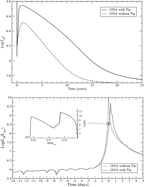
Figure 10: Evolutionary time-scales during the born-again event for sequences computed with the GNA convection theory with and without the effects of $\nabla\mu$ included in the calculation of the mixing coefficient $D$ (top panel). Evolution of $L_{\rm H}$ during the development of the H-flash (bottom panel). The influence of $\nabla\mu$ becomes noticeable only when the second stage of proton burning sets in. The effects of $\nabla\mu$ become important as material with lower $\mu$ is rapidly injected into the burning shell, slightly delaying the violent increase of $L_{\rm H}$. The inset shows the small effect of the molecular weight gradient in the energy release distribution.

Next, we analyze the effect of chemical inhomogeinities in the convective shell during proton burning. To this end we compare the two sequences calculated with the GNA theory (one including the effect of $\nabla\mu$, and the other by setting $\nabla\mu=0$ in the calculation of $D$). A comparison of these sequences is shown in Fig. 10. During the first stage of the onset of proton burning, the amount of protons ingested in the convection zone is relatively small and $\nabla\mu$ is not significant to alter the value of $D$. Thus, the presence of $\nabla\mu$ does not change the evolution of this stage of proton burning. However, during the second stage of proton burning, larger quantities of H are rapidly transported downwards, causing $\nabla\mu$ to be larger. A positive $\nabla\mu$ tends to favour convective stability, resulting in a lower value of $D$ than if $\nabla\mu$ is assumed to be zero. In addition, a smaller value of $D$ implies lower rates of proton burning, leading to a lower value of ($\nabla_{\rm rad}-\nabla_{\rm ad}$) which in turn increases the difference between $D$ and $D(\nabla\mu=0)$. As a result of this slight reduction in $D$ at the PBCZ, proton burning becomes somewhat less violent and lower values of $L_{H}$ are attained (bottom panel of Fig. 10), with the consequence that the born again times are larger (upper panel of Fig. 10). Note that this is not related to the location of the peak of proton burning, which is not affected by the inclusion of $\nabla\mu$ (because $\nabla\mu$ is not important until the start of the second stage of proton burning).

4.4 Effect of the overshooting parameter $f$

To explore the role of the overshoot parameter $f$, we have calculated an additional MLT-sequence with $f=0.03$ . It may be argued that changing $f$ only at the VLTP stage is not consistent with the prior evolution. We do not expect, however, this inconsistency to alter the main aspects of the following discussion. In fact, there is no reason to believe that the overshooting efficiency during the extreme conditions characterizing the VLTP should remain the same as that prevailing during prior evolutionary stages. Interestingly enough, we find that born-again evolution is sensitive to the adopted $f$.

Figure 11: Location of the peak of the energy liberated by proton burning at selected stages during the ingestion of protons for different values of the overshooting parameter $f$. Solid lines show the diffusion coefficient and the energy liberated (per unit time and mass) for the model with $f=0.016$ while dashed lines show the situation for $f=0.03$ (thin lines correspond to log$D$ and thick lines log$\epsilon$). Upper left: just before the splitting of helium flash convection zone as a consecuence of the energy generated by proton burning. Upper right: when the convective region has just splitted into two. Bottom left: the situation at the maximum of $L_{H}$. Bottom right: after the maximum of proton burning.

The sequence with increased overshooting efficiency takes about 20 yr to reach $\log{T_{\rm eff}}\sim 3.8$, as compared to the 10 yr employed by the $f=0.016$ sequence. The reason for the slower evolution in the $f=0.03$ case can be understood by examining the evolution of the locus of maximum proton burning during the ingestion of protons as shown in Fig. 11. Note that, while in both sequences the peak of proton burning (and the moment of the splitting of the convective zones) starts to develop at about the same position (in mass) at $m\sim 0.58$ M_⊙, the situation changes soon. In fact, for the sequence with $f=0.016$ the peak of proton burning moves downwards only to $m\sim 0.579$ M_⊙ as the energy released by proton burning increases, but for the case with $f=0.03$ it progressively sinks into deeper regions of the star, reaching a mass depth of 0.577 M_⊙ by the time $L_{H}$ has reached its maximum value. A larger overshooting efficiency allows protons to reach deeper layers, below the inner boundary of the PBCZ. This has the effect of shifting the maximum nuclear energy release to inner regions that become unstable to convection because of the high luminosity. The net effect, as mentioned above, is a final displacement in the peak of proton burning to deeper regions of the star by more than 0.003 M_⊙ in mass. Correspondingly, evolutionary time-scales are longer.

An issue raised by the referee is concerning the possibility that the overshooting mixing at the H-He interface could be attenuated by the stabilizing effect of the chemical gradient. To analyze this possibility we have calculated two more GNA-sequences under the $extreme$ situation in which no overshooting is present at the outer border of the He-driven convection zone (OBHeCZ). Under this assumption our two sequences display a very different behavior. In the 2.7 M_⊙ sequence, which suffers from an early-VLTP and in which some entropy barrier is still present, the presence of $\nabla\mu$ prevents the He-driven convection zone from reaching the H-rich envelope. Thus in this sequence H-burning was inhibited. On the other hand in the 2.5 M_⊙ sequence (in which proton burning is almost completely extinguished at the moment of the He-flash) the $\nabla\mu$-barrier is not enough to prevent proton burning. However evolution proceeds differently from the case in which overshooting mixing was present. First the starting of proton ingestion was delayed for about 10 days. Then, once the ingestion of protons has started, as consequence of $\nabla\mu$ some semiconvective regions develop that split the OBHeCZ into separate convective regions. Then H is premixed in the more external convective regions before being ingested and burned. As a result, log$(L_{H}/L_{\odot})$ remains below 7 for about half year delaying the start of the second (runaway) stage of proton burning. Only when $L_{H}$ has became high enough and the H-abundance in the pre-mixed convective regions has been lowered are these convective regions reconnected. Then, due to this change in the way protons are burned the born again times change, being much larger (about 100 yr) than in the case in which overshooting was considered.

4.5 Miscellanea

Our evolutionary results do not indicate the need of a strong reduction in mixing coefficient $D$ to achieve born-again time-scales comparable to the rapid evolution showed by the Sakurai’s object. However, a reduction in $D$ certainly leads to faster born-again evolution. As it is show in Fig. 5 a $slight$ reduction in the mixing efficiency by a factor of 3 shortens the born again time to about 3 years.

We have perfomed additional VLTP computations to assess the possibility that our conclusions could be affected by other numerical resolution issues. We find no dependence of our born-again time-scales on the chemical time step used in the integration of the chemical evolution. Nor do we find any significant dependence on the adopted mesh resolution. Also as explained in Appendix A, two different approaches for the linearization of the structure equations were used in the calculations, and no significant difference in the born again times was found. Additionally, we explored the effect of possible uncertainties (of about 10% to 20%) in the rate of the ${}^{12}{\rm C}+p\rightarrow^{13}{\rm N}+\gamma$. Again, we find no relevant effect on the born again times.

5 Comparison with observations and chemical evolution of the models

5.1 Pre-Outburst parameters

Figure 12: Comparison of our standard model (section 3) with the preoutburst properties derived from observations. Grey dashed line corresponds to the possible detection at m_j=21 in 1976 (taken from Herwig 2001), if a distance of 4 Kpc is assumed. Crosses mark the location of Sakurai’s object and V605 Aql previous to the helium flash as derived from photoionization models (Pollaco 1999 and Kerber et al. 1999 for Sakurai’s object and Lechner & Kimeswegner 2004 for V605 Aql. Inset: Evolution of surface abundances. Note the change in the surface H while the other elements remain unchanged. A similar behavior in the surface abundances has been reported in Sakurai’s object during 1996 (Asplund et al. 1999). Black dots mark the location in the HR before and after the second change in the H-abundance.

In Fig. 12 we compare the HR-locus of the model at the moment of the He-Flash with that derived from photoionization models for Sakurai’s object and V605 Aql (Pollaco 1999, Kerber et al. 1999 and Lechner & Kimeswenger 2004), and with the possible detection of Sakurai’s object as a faint object of $m_{J}\sim 21$ on the J plate of the ESO/SERC sky survey taken in 1976 (Duerbeck & Benetti 1996, Herwig 2001). As it is shown in Fig. 12 our model shows a good agreement with the possible detection at $m_{J}\sim 21$ when a distance of 4 Kpc is assumed. Comparison with photoinoization models shows a relatively good agreement, in particular when a distance scale (which determines the zero point of the y-axis of the observations) between 5 Kpc and 1.5 Kpc is chosen.

5.2 Evolution of effective temperature and luminosity

In Fig. 5 we show the temporal evolution of the luminosity and the temperature for both the theoretical models and the observed parameters of Sakurai’s Object (Duerbeck et al. 1997, Asplund et al. 1999). Although important quantitative disagreement exists with observations, some of the observed features of Sakurai’s object are predicted by the models. Indeed note that the cooling rate of the models is similar to the observed one. When comparing the timescales of V4334 Sgr with those of the models, we have to keep in mind that the observed born again times are measured from the moment the object has become bright enough (and not from the moment of the flash itself). The light curve of our models during the first years after the violent proton burning is roughly similar to the observed one, that is, the object increases its luminosity by more than 2 orders of magnitude in less than a year (Fig.5), in agreement with the observed one (Duerbeck et al. 1997, Duerbeck et al. 2002).In addition the log($L/L_{\odot})$ value of 3.5-3.7 predicted by our models after the outburst is similar to the luminosity derived for V4334 Sgr (by Duerbeck and Bennetti 1996) when a conservative distance scale of 5.5 kpc is adopted (log$(L/L_{\odot})\sim 3.49$, $T_{\rm eff}\sim 3100$). On the other hand our models are incompatible with the luminosity of 10000 $L_{\odot}$ derived when adopting the long distance scale (8 kpc, Duerbeck et al 1997).

On the other hand our models fail to reproduce the quick reheating (less than 6 years after reaching log$T_{\rm eff}\sim 3.8$) shown by Sakurai’s object as reported by Hajduk et al. (2005). This could be probably related to the fact that the hydrostatical hypothesis assumed in our modeling is explicitly broken in the outer regions of the star. In this connection let us note that although Hajduk et al. (2005) claim that this feature can be reproduced by means of models with a high supression of the mixing efficiency, we think that this has to be taken with a pinch of salt. The lowest log$(T_{\rm eff})$ reached by the model presented in that work is 3.95 and thus can not reproduce the observed evolution of the Sakurai’s Object effective temperature, that has reached values as low as log$(T_{\rm eff})\sim$3.8. Also notice that it is below log$(T_{\rm eff})=3.8$ that we find that hydrodynamical effects in the envelope become important, and ejection of envelope material is likely to occur. In connection with this, it is worth mentioning that the Sakurai’s Object has been observed to go through a massive dust shell phase when its effective temperature was below log$(T_{\rm eff})=3.8$ (Duerbeck et al. 2000).

Figure 13: Inner Chemical evolution. Panel A shows the chemical profile before the onset of proton ingestion (He burning is located at about log$(q)$=-1.37). Note that almost all the previously created ¹⁴N has been destroyed. Panel B shows the interior of the models at the maximum of proton burning, which has its maximum intensity near log$(q)$=-1.88. Note especially the inhomogenous distribution of H at the PBCZ (which at that moment ranges from -1.88 to -4.9). Also see the creation of ¹³C and ¹⁴N due to the ingestion of protons. Finally last panel shows the chemical abundances somewhat later when the model start to cool as consequence of the expansion of its outer layers. At that moment the envelope is almost homogenous as a consequence of convection, but the H-abundance left by proton burning displays a marked depth dependence.

5.3 Chemical evolution of the models

In Fig. 13 the evolution of the abundance distribution within the star during the VLTP is shown. Until the ingestion of protons, the chemical abundance distribution is essentially that of its AGB predecesor. During the VLTP, the outwards growing helium flash convection zone penetrates into the helium buffer, and as a result the ¹⁴N left behind by CNO reactions in the helium buffer is burned into ²²Ne. This leads to an almost total depletion of ¹⁴N in the He convective zone. The course of events up to this point is similar to that occurring during the thermally pulsing AGB phase, but things change as soon as protons are ingested into the convective region. Initially the ingestion of protons causes only an increase in ¹³C. This continues until the convection region splits into two and unstable proton burning develops. A few hours after the splitting of the convective region, when enough quantities of ¹³C have been produced, the reaction ¹³C(p,$\gamma$)¹⁴N takes over and the amount of ¹⁴N in the PBCZ increases. Also after proton burning has reached its maximum extent, ¹⁴N and ¹³C, which had initially a maximum abundance at the place of major proton burning are soon homogenized by convection in the whole PBCZ (last panel of Fig. 13). This process leads to an important ¹⁴N abundance in contrast with what would be expected in a Late Thermal Pulse (LTP), where most ¹⁴N abundance is destroyed during the He flash and never recovered.

	H	He	C	N	O	$M^{total}_{H}/M_{\odot}$
MLT (early VLTP)	$3.7\times 10^{-4}$	0.324	0.371	0.0145	0.217	$3.19\times 10^{-6}$
MLT ($f=0.03$)	$5\times 10^{-6}$	0.307	0.378	0.0129	0.229	$7.24\times 10^{-9}$
GNA ($\nabla\mu=0$)	$3.2\times 10^{-5}$	0.316	0.378	0.0129	0.221	$2.19\times 10^{-7}$
GNA	$3.3\times 10^{-5}$	0.316	0.378	0.0127	0.221	$6.76\times 10^{-9}$
Lawlor $D/10^{-4}\dagger$	0.06	0.57	0.26	-	0.07	$2\times 10^{-6}$
Lawlor $D/10^{-3}\dagger$	0.02	0.55	0.28	-	0.08	$3\times 10^{-7}$
Lawlor $D/10^{-2}\ddagger$	0.04	0.54	0.28	-	0.08	-
Herwig(1999)	-	0.388	0.362	-	0.219	$4\times 10^{-11}$
Most PG1159 pulsators	-	0.397	0.357	0.0139	0.159	-
PG1159-035	-	0.287	0.516	0.0100	0.115	-

Table 2: Surface abundances of the models presented in Sect. 4. Abundances are taken at the moment the models reach the giant region for the first time after the VLTP. Abundances from Lawlor & Macdonald (2003) are taken from models of similar metallicity (z=0.02) $\dagger$ Abundances correspond to the moment at which the star reaches the WD cooling track. $\ddagger$ Abundances correspond to the first return to the giant region, where the envelope was homogeinized by mixing. In the last column the values of the total amount of H in the star after the VLTP are presented. Relative abundances of PG1159 stars are taken from Dreizler & Heber (1998) and normalized to the total amount of C+O+N+He given by the models.

5.3.1 Surface Abundances

In all of our calculations the internal solutions (of the Henyey iteration) were calculated up to a fitting mass fraction $\xi_{1}=$ln$(1-{m_{r}}/{M_{\star}})=-20$ during the proton burning and the first years after it (with the exception of the sequence shown in Fig. 8 and 10, where $\xi_{1}=-12$ ). This means that approximately $2\times 10^{-9}\,M_{\star}$ are left out of chemical integration. Even though this is enough to account for the gravothermal energy generated in the outer layers of the star, it may be still not small enough to follow in detail the chemical evolution that takes place in the outermost surface of the star. This prevents us from making a detailed comparison with the observed abundances of Sakurai’s object. Indeed, convective dilution as well as modest mass loss rates in the giant state are expected to erode the last vestiges of H left in the star after the born-again chemical processing, exposing the underlying H-deficient layers. Nonetheless, we can still try to compare the abundances characterizing the envelope of our models with those of the PG 1159 stars and V4334. The values of the surface abundances (i.e. the mass fraction at the outermost shell of the interior) of our models is presented in Table 2 (for those calculated with a MTS of $10^{-5}$ yr). Note that our surface abundances are [He/C/O]=[0.38/0.36/0.22], in agreement with those obtained by Herwig (1999). Also the abundances presented in Table 2 are similar to surface abundance patterns observed in PG1159 stars ([He/C/O]=0.33/0.50/0.17]) Dreizler & Heber (1998), but with a lower abundance of He and C, and a larger amount of oxygen. These differences in the abundances of He and O may be taken as a signal that the overshoot parameter $f$ is a bit smaller than the one used here. In fact, lower overshoot efficiency yields lower oxygen abundances in the intershell region during the thermally pulsing AGB phase (Herwig 2000). Also it is expected that intershell abundances may depend on the mass of the remnant. It is worth noting the remarkably good agreement between the ¹⁴N abundances of our models and those observed in pulsating PG1159 stars (Dreizler & Heber 1998). This makes these objects more likely to be produced by a VLTP, in contrast with the situation for nonpulsators PG1159 which do not show ¹⁴N features at their surface. As it is shown in Table 2 in all of the calculations (with different numerical and physical parameters) we obtain stellar models that display a surface ¹⁴N mass abundance of 0.01. This is exactly what it is observed in PG1159 pulsators (and also on V4334 Sgr). This reinforces the idea that PG1159 pulsators would have experienced a VLTP in the past. On the other hand PG1159 nonpulsators could have followed a different evolutionary channel, for instance a LTP (in which hydrogen is only diluted as a consequence of the He flash, and no ¹⁴N is produced). It is worth noting in view of the discussion presented by Vauclair et al. (2005), that in no one of the sequences we performed here an He-enriched surface composition with no detectable nitrogen was obtained (typical composition of PG1159 nonpulsators). One may be tempted to think that if stellar winds were stronger during the pre-PG1159 evolution models with no trace of ¹⁴N could be obtained, but this mechanism would not lead to a He-enriched surface.

In Fig. 12 we show that our models predict a second change in the surface abundance of H (the first happened during violent proton burning), while the other elements remain almost unchanged. This takes place when the star reaches the giant region and a convective envelope starts to develop (see Fig. 2). As a result of the non instantaneous mixing at the (short lived) PBCZ, H abundance varies with depth (with higher amounts of H at the top). Thus when the envelope starts to mix due to convection the surface abundance of H is diluted and its value drops by more than an order of magnitude. This is qualitatively similar to the observed behavior of the surface abundances in Sakurai’s object during 1996 (Asplund et al. 1999), before it dissapeared as consequence of dust episodes in 1998.

We note that lower values of $D$ increase the amount of He and lower the surface oxygen. This is expected because mixing of material becomes less eficient with a lower $D$. As was noted by Lawlor & MacDonald (2003), we also find that when the value of $D$ is reduced by a factor of 100, the H abundance remaining at the surface of the star is not consistent with the ones observed at the Sakurai’s object. Although, this inconsistency may be due to the fact that we are not taking into account mass loss. Finally, we note that models with small convective efficiency are characterized by surface ¹⁴N abundances somewhat smaller than observed.

6 Final remarks and conclusions

In this paper we have studied the born again scenario for 0.5842 and 0.5885 M_⊙ model star, under several numerical and physical assumptions. For consistency purposes the VLTP initial stellar models have been obtained following the complete evolution of initially 2.5 and 2.7 $M_{\odot}$ stellar models, from the ZAMS through the thermally pulsing AGB phase. We incorporate an exponentially decaying diffusive overshoot above and below any formally convective border during the whole evolution. The inclusion of a time-dependent scheme for the simultaneous treatment of nuclear burning and mixing processes due to convection, salt finger and overshoot has allowed us a detailed study of the abundance changes over all the evolutionary stages. Also we incorporate in our study the double diffusive GNA convection theory for fluids with composition gradients, which allows us to study the role of the chemical gradients.

In the present work we have found that, according to our treatment of mixing and burning, born again times are very sensitive to the adopted time resolution during the proton ingestion, and that these times converge to a given value when we keep the minimum allowed time step (MTS) below $\sim 5\times 10^{-5}$ For the sequences calculated with MTS $\mathrel{\hbox{\hbox to0.0pt{\hbox{\lower 4.0pt\hbox{$\sim$}}\hss}\hbox{$<$}}}5\times 10^{-5}$ we find that:

• The inclusion of $\nabla\mu$ in the calculation of the mixing velocity during the violent proton burning leads to an increase in the born again times by about a factor of 2. This leads to born again times of 10-20 yr which are not consistent with the observed born again time of Sakurai’s Object.

• One interesting point of the present work is that we find, with the standard mixing length theory (i.e. not considering $\nabla\mu$ in the calculation of mixing velocities), very short born again times of 5-10 years (that is of the order of magnitude of those observed in V605 Aql and V4334 Sgr) even in the case that no reduction in the mixing efficiency is invoked. Our born again times are then closer (although shorter) to the ones originally found by Iben & MacDonald (1995).

Also other important results of the present work are:

• We find that proton ingestion can be seriously altered if the occurence of overshooting is modified by the $\nabla\mu$-barrier at the H-He interface, and thus changing the born again times.

• Also we find that saltfinger instability regions develop below the proton burning convective zone. The occurrence of such instability regions bears no consequences for the further evolution of the star, particularly the evolutionary timescales.

• A detailed description of the development of proton burning has been provided. In particular we identify two different stages of the proton ingestion.

• We have compared the evolution of the surface parameters of the models with those observed in Sakurai’s Object and we find that, although born again times are larger than the observed, both luminosity curve and the surface cooling rate show a qualitative agreement with those observed in Sakurai’s Object. Also the drop in the H abundance (with no significant change in the other chemical species) observed during 1996 in Sakurai’s object is qualitatively predicted by our models.

We close the paper by mentioning some of the work that need to be done before we can finally understand the VLTP scenario. In particular an assessment of the influence of the AGB progenitor evolution (particularly regarding the number of thermal pulses experienced by the progenitor star) on the born again times would be valuable. Also calculations of VLTPs including a simultaneous resolution of both structural and composition equations are needed. But more importantly a more detailed treatment of convection than the local and one dimensional approach attempted here is necessary. In this connection two items should be studied. First a detailed study of the interaction of chemical gradients and overshooting mixing is in order. Second, as the timescale during H-ingestion is of the order of magnitude of the convective turn over timescale, it would be necessary to explore the H-flash on timescales at and below the convective turn over timescale and to study convection away from the diffusion limit.

Appendix A Two Linearization Schemes for Stellar Structure Equations

An appropriate choice of the linearization scheme of the equations of stellar structure can be of crucial importance in certain evolutionary stages. In order to determine the importance of such a choice in the case of the born-again scenario, two intrinsically different schemes were used.

Following the notation of Sugimoto (1970), we write the four evolution equations as

$${\partial y_{i}}/{\partial x}=\phi(x,\@vec{y}),$$ (5)

where we denote by $y_{i},\,i=1,2,3,4$ the dependent variables $\ln{p}$, $\ln{T}$, $\ln{r}$ and $L$ (here $p$, $T$, $r$ and $L$ have their usual meaning) and by $x$ the independent variable related to the fractional mass.

The first aproach is the one proposed by Sugimoto (1970) for rapid evolutionary phases, generally characterized by negative temperature gradients like those developed during shell flashes below the point of maximum energy release. Here, the finite difference equations are written as:

$${y_{i}}^{k+1}-{y_{i}}^{k}=\Delta x^{k}\left[\beta_{i}\phi_{i}(y^{k},x^{k})+(1-\beta_{i})\phi_{i}(y^{k+1},x^{k+1})\right]$$ (6)

where $\beta_{1}=\beta_{3}=1/2$, $\beta_{2}=1$ and $\beta_{4}=0$. This means that the derivatives of $\ln{T}$ and $L$ between the mesh points $k+1$ and $k$ are approximated by their values at these points. As shown by Sugimoto (1970) this representation leads to a more stable scheme during rapid evolutionary phases (as it is the case for the born again scenario). The gain in stability is at the expense of a loss in accuracy, which can be troublesome when long evolutionary steps are used. However, as shown by Sugimoto (1970), when the time-step is small enough, the accuracy of the usual implicit scheme ($\beta_{i}=1/2$ for all $i$) is recovered. The time-scale associated with the born-again phase, ensure that the evolutionary time-step always remain small, and the accuracy of the method is then granted.

The second linearization scheme is based on the representation of the finite-difference equations in two grids of mesh points in a de-centered way. Specifically, on the first grid $x_{j}$ ($j=1,...,N$), we evaluate $L$ and $\ln{r}$, while $\ln{p}$ and $\ln{T}$ are specified on a pseudo-grid ($j^{\prime}=1,...,N$), defined by $x_{j^{\prime}}=(x_{j}+x_{j-1})/2$ for $j^{\prime}=2,...,N-1$ and by $x_{1^{\prime}}=x_{1}$ and $x_{N^{\prime}}=x_{N}$ (surface and center respectively). Accordingly, the equations are written as:

$${y_{i}}^{k^{\prime}}-{y_{i}}^{k^{\prime}-1}=\Delta x^{k^{\prime}}\phi_{i}(\frac{{y_{1}}^{k^{\prime}}+{y_{1}}^{k^{\prime}-1}}{2} \frac{{y_{2}}^{k^{\prime}}+{y_{2}}^{k^{\prime}-1}}{2}$$ ,

$$,{y_{3}}^{k-1} {y_{4}}^{k-1},x^{k-1})$$ , (7)

for $i=1,2$, and

$${y_{i}}^{k}-{y_{i}}^{k-1}=\Delta x^{k}\phi_{i}({y_{1}}^{k^{\prime}} {y_{2}}^{k^{\prime}},\frac{{y_{3}}^{k}+{y_{3}}^{k-1}}{2}$$ ,

, $$\frac{{y_{4}}^{k}+{y_{4}}^{k-1}}{2},\frac{x^{k}+x^{k-1}}{2})$$

for $i=3,4$. This method has the advantage that all the derivatives have information from two mesh points while at the same time it is very robust and does not give rise to unphysical solutions as those found with the usual implicit scheme in certain evolutionary phases as mentioned above. This is our preferred choice for linearizing the stellar structure equations.

In practice, born-again calculations were carried out using both schemes just described. The time-scales found with both schemes, while keeping the physical inputs and other numerical issues (see Sect. 2.2) the same, were in all our tests very similar, the differences being smaller than 10%, and the absolute time-scale being determined solely by the choice of the minimum time-step.