Non-linear axisymmetric pulsations of rotating relativistic stars in the conformal flatness approximation

Abstract

We study non-linear axisymmetric pulsations of rotating relativistic stars using a general relativistic hydrodynamics code under the assumption of a conformally flat three-metric. We compare the results of our simulations, in which the spacetime dynamics is coupled to the evolution of the fluid, to previous results performed in the Cowling approximation in which the spacetime dynamics was neglected. We show that the conformal flatness condition has only a small effect on the dynamics of pulsating relativistic stars and the obtained pulsation frequencies are very close to those expected in full general relativity. The pulsations are studied along various sequences of both uniformly and differentially rotating relativistic polytropes with index $N=1$. For small pulsation amplitudes we identify several modes, including the lowest-order $l=0$, 2, and 4 axisymmetric modes, as well as several axisymmetric inertial modes. Differential rotation significantly shifts mode frequencies to smaller values, increasing the likelihood of detection by current gravitational wave interferometric detectors. We observe an extended avoided crossing between the $l=0$ and $l=4$ first overtones (previously known to exist from perturbative studies), which is important for correctly identifying mode frequencies in case of detection. For uniformly rotating stars near the mass-shedding limit, we confirm the existence of the mass-shedding-induced damping of pulsations and argue that it is still relevant for secularly unstable modes, even though the effect is not as strong as was previously found in the Cowling approximation. We also investigate non-linear harmonics of the linear modes and notice that rotation changes the pulsation frequencies in a way that would allow for various parametric instabilities between two or three modes to take place. Although this scenario has been explored before for slowly-rotating collapse, it could become very interesting in the case of rapidly rotating collapse, where the quasi-radial mode could be in resonance with inertial modes. We assess the detectability of each obtained mode by current gravitational wave detectors and outline how the empirical relations that have been constructed for gravitational wave asteroseismology could be extended to include the effects of rotation.

1 Introduction

Axisymmetric pulsations of rotating neutron stars could be excited in a number of astrophysical scenarios, such as rotating core collapse, accretion-induced collapse, core quakes due to a large phase-transition in the equation of state (EOS), or hypermassive neutron star formation in a binary neutron star merger (see Stergioulas, Apostolatos & Font, 2004; Kokkotas & Stergioulas, 2005, for extensive discussions). These pulsations are a potential source of detectable high-frequency gravitational waves. While for nonrotating stars the frequencies of normal modes can be computed with perturbative methods and a theory of gravitational wave asteroseismology has already been formulated (Andersson & Kokkotas, 1998; Kokkotas, Apostolatos & Andersson, 2001; Benhar, Ferrari & Gualtieri, 2004), there exist no accurate frequency determinations for rapidly rotating stars to date, nor has the theory of gravitational wave asteroseismology been extended to include the effects of rotation on the oscillation frequencies. Most existing computations of oscillation modes in rapidly rotating relativistic stars use the Cowling approximation (Yoshida et al., 2002; Stergioulas, Apostolatos & Font, 2004; Yoshida, Yoshida & Eriguchi, 2005), with the only exception being the computation of the two lowest-order quasi-radial modes in Font et al. (2002) (see also Shibata, 2003; Shibata & Sekiguchi, 2003).

In this paper we present an accurate determination of several axisymmetric pulsation modes of rotating stars in general relativity. The accurate knowledge of the frequencies of different modes excited in the astrophysical events mentioned above is necessary both for narrow-banding of the detectors, as well as for solving the inverse problem, i.e. identifying the EOS of high-density matter.

The traditional approach for computing mode frequencies uses perturbation theory for either solving a time-independent eigenvalue problem or for obtaining the time evolution of the linearised equations governing the dynamics of matter and spacetime (see Kokkotas & Schmidt, 1999; Kokkotas & Ruoff, 2003, for comprehensive reviews of these approaches). The advantage of the perturbative approach is that the equations can be expanded in terms of spherical harmonics. However, for rapidly rotating relativistic stars this approach has only worked in the Cowling approximation so far (Yoshida & Eriguchi, 1999, 2001; Yoshida et al., 2002; Yoshida, Yoshida & Eriguchi, 2005), except for zero-frequency $f$-modes, which were computed in full general relativity (Stergioulas & Friedman, 1998; Morsink, Stergioulas & Blattnig, 1999). The main problem for applying the perturbative approach in full general relativity is the absence of analytic boundary conditions at infinity, which would allow to apply the outgoing-wave boundary conditions defining the quasi-normal modes (see Stergioulas, 2003, for a review). Only if one assumes the slow-rotation approximation the problem is still tractable (see, e.g., Hartle & Friedman, 1975; Kojima, 1997; Datta et al., 1998; Ruoff & Kokkotas, 2002; Pons et al., 2005).

In recent years, the time evolution of the non-linear equations governing the dynamics of matter and spacetime has been introduced as a promising new approach for computing mode frequencies (Font, Stergioulas & Kokkotas, 2000; Font et al., 2001, 2002; Stergioulas & Font, 2001; Stergioulas, Apostolatos & Font, 2004). For small amplitudes, the obtained frequencies are in excellent agreement with those expected by linear perturbation theory, while two-dimensional eigenfunctions can be obtained through a Fourier transform technique (see Stergioulas, Apostolatos & Font, 2004, SAF hereafter). The advantages of this method are that one does not need precise outer boundary conditions and that one can also study non-linear pulsations.

This study extends the results presented in SAF (which were obtained in the Cowling approximation) by incorporating the spacetime dynamics in the evolutions. This is done by using the Isenberg–Wilson–Mathews approximation of general relativity (also known as the conformal flatness condition; hereafter CFC) where the 3 + 1 Einstein equations reduce to a non-linear set of five coupled elliptic equations for the lapse function, the shift vector, and the conformal factor (Isenberg, 1978; Wilson, Mathews & Marronetti, 1996). The approximation essentially ignores gravitational radiation and is thus appropriate for equilibrium, quasi-equilibrium, but also for highly dynamical situations (see, e.g., Cook, Shapiro & Teukolsky, 1996; Dimmelmeier, Font & Müller, 2002a; Oechslin, Rosswog & Thielemann, 2002; Faber, Grandclément & Rasio, 2004; Saijo, 2004).

For small pulsation amplitudes we identify several modes, including the lowest-order $l=0$, 2, and 4 axisymmetric modes as well as several axisymmetric inertial modes. The pulsations are studied along the same sequences of uniformly and differentially rotating relativistic polytropes with index $N=1$ as in SAF. Differential rotation significantly shifts mode frequencies to smaller values, increasing the likelihood of detection by current gravitational wave interferometric detectors. An important feature of the frequency spectrum, induced by rotation, is the existence of avoided crossings between different mode sequences (see Clement, 1986; Yoshida & Eriguchi, 2001). We observe an extended avoided crossing between the $l=0$ and $l=4$ first overtones. This is important for correctly identifying mode frequencies in case of detection.

Our non-linear approach allows us to identify non-linear harmonics in addition to the well known linear modes. These harmonics arise due to couplings between various modes or due to non-linear self-couplings (see also Sperhake, Papadopoulos & Andersson, 2001; Sperhake, 2002); for similar results obtained for the non-linear oscillations of a torus orbiting a black hole, see Zanotti et al. (2005). It has been suggested (Clark, 1979; Eardley, 1983) that nonradial oscillations after core bounce could be enhanced through a parametric instability with the quasi-radial mode (see also Passamonti et al., 2005, for recent related work). In nonrotating or slowly rotating collapse, such a parametric instability can only take place under special conditions that would allow the two modes to be in resonance. In our work we find that rotational shifting of the frequency of different modes broadens the range of parameters for which interesting resonances could take place. In particular we notice that the quasi-radial mode will be in resonance with some inertial mode(s) for all rotation rates above a critical value. It is thus interesting to further study the possible energy transfer between different modes excited after, e.g., a core collapse or an accretion-induced collapse event, either on secular time-scales or as a possible parametric instability.

The paper is organized as follows. In Section 2 we introduce the mathematical and numerical framework and specify the initial fluid perturbations, while in Section 3 we present the sequences of equilibrium initial models. In Section 4 we discuss the effects of linear pulsations, focusing on the role of rotation and avoided crossings of modes, and present a detailed comparison to results in the Cowling approximation. Section 5 is devoted to the technique of mode recycling, and in Section 6 we examine non-linear effects of the pulsations like mode coupling or mass-shedding-induced damping. Gravitational wave emission and asteroseismology are discussed in Section 7. A summary of our results in Section 8 concludes this work.

Unless otherwise noted, we choose dimensionless units for all physical quantities by setting the speed of light, the gravitational constant, and the solar mass to one, $c=G=M_{\odot}=1$. Latin indices run from 1 to 3, Greek indices from 1 to 4.

2 Mathematical and numerical framework

We study axisymmetric pulsations of rapidly rotating relativistic stars by first constructing several sequences of uniformly and differentially rotating equilibrium models. In SAF the equilibrium models were constructed using the numerical code rns (Stergioulas & Friedman, 1995). In the present work we build the stellar equilibrium models using the self-consistent field method described in Komatsu, Eriguchi & Hachisu (1989a, b) (KEH hereafter), which solves the general relativistic hydrostatic equations for rotating matter distributions whose pressure obeys an EOS given by a polytropic relation (see Eq. (9) below). Comparisons of the accuracy of both approaches in the case of uniform rotation can be found in Nozawa et al. (1998) and in Stergioulas (2003). Specific details of the equilibrium models are deferred to Section 3 below, where a quantitative comparison of the equilibrium properties of a particular highly differentially rotating model built either using rns or the KEH solver is made.

These equilibrium models are taken as initial data for the evolution code after a suitable perturbation has been added in order to excite specific modes of oscillation (see Section 2.4). The time dependent numerical simulations are performed with the code CoCoNuT, developed by Dimmelmeier, Font & Müller (2002a, b) with a metric solver based on spectral methods as described in Dimmelmeier et al. (2005). The code uses the general relativistic field equations for a curved spacetime in the 3 + 1-split under the assumption of conformal flatness for the three-metric. The hydrodynamics equations are consistently formulated in conservation form, and are solved by high-resolution shock-capturing schemes.

In the code used by SAF, the spacetime dynamics was neglected, and the attention was focused on the oscillations of the stars on a fixed background metric given by the solution of the Einstein equations on the initial time slice. Keeping the spacetime fixed to the initial equilibrium state during the evolution corresponds to the Cowling approximation in perturbation theory. In the simulations presented in this work, however, such a simplification is not made and the spacetime fields are also allowed to evolve in time.

In the following, we present the mathematical formulation of the metric and hydrodynamics equations, and then summarise the numerical methods used for solving them.

2.1 Metric equations

We adopt the ADM 3 + 1 formalism by Arnowitt, Deser & Misner (1962) to foliate a spacetime endowed with a metric $g_{\mu\nu}$ into a set of non-intersecting spacelike hypersurfaces. The line element then reads

$$ds^{2}=g_{\mu\nu}\,dx^{\mu}\!dx^{\nu}=-\alpha^{2}dt^{2}+\gamma_{ij}(dx^{i}+\beta^{i}dt)(dx^{j}+\beta^{j}dt),~{}$$ (1)

where $\alpha$ is the lapse function, $\beta^{i}$ is the spacelike shift three-vector, and $\gamma_{ij}$ is the spatial three-metric.

In the 3 + 1 formalism, the Einstein equations are split into evolution equations for the three-metric $\gamma_{ij}$ and the extrinsic curvature $K_{ij}$, and constraint equations (the Hamiltonian and momentum constraints) which must be fulfilled at every spacelike hypersurface:

$$\begin{array}[]{rcl}\partial_{t}\gamma_{ij}&=&-2\alpha K_{ij}+\nabla_{\!i}\beta_{j}+\nabla_{\!j}\beta_{i},\\[8.00003pt] \partial_{t}K_{ij}&=&-\nabla_{\!i}\nabla_{\!j}\alpha+\alpha(R_{ij}\!-\!2K_{ik}K_{j}^{k})+\beta^{k}\nabla_{\!k}K_{ij}+K_{ik}\!\nabla_{\!j}\beta^{k}\\[5.0pt] &&\displaystyle+K_{jk}\nabla_{\!i}\beta^{k}-8\pi\alpha\!\left(\!S_{ij}-\frac{\gamma_{ij}}{2}(S_{k}^{k}-\rho_{\mathrm{H}})\right),\\[8.00003pt] 0&=&R-K_{ij}K^{ij}-16\pi\rho_{\mathrm{H}},\\[8.00003pt] 0&=&\nabla_{\!i}K^{ij}-8\pi S^{j},\end{array}$$ (2)

where the maximal slicing condition, $K^{i}_{i}=0$, is imposed. In these equations $\nabla_{\!i}$ is the covariant derivative with respect to the three-metric $\gamma_{ij}$, $R_{ij}$ is the corresponding Ricci tensor, and $R$ is the scalar curvature.

The matter fields of the general relativistic fluid appearing in the above equations are the spatial components $S_{ij}$ of the (perfect fluid) stress-energy tensor $T^{\mu\nu}=\rho hu^{\mu}u^{\nu}+Pg^{\mu\nu}$, the three momenta $S^{i}=\rho hW^{2}v^{i}$, and the total energy $\rho_{\mathrm{H}}=\alpha^{2}T^{00}$. The fluid is specified by the rest-mass density $\rho$, the four-velocity $u^{\mu}$, and the pressure $P$, with the specific enthalpy defined as $h=1+\epsilon+P/\rho$, where $\epsilon$ is the specific internal energy. The three-velocity of the fluid as measured by an Eulerian observer is given by $v^{i}=u^{i}/(\alpha u^{0})+\beta^{i}/\alpha$, and the Lorentz factor $W=\alpha u^{0}$ satisfies the relation $W=1/\sqrt{1-v_{i}v^{i}}$.

The equations of the original ADM formulation, when implemented numerically with standard finite-difference methods, suffer from several numerical instabilities. For many years there have been numerous attempts to reformulate these equations into forms better suited for numerical work (see, e.g., Alcubierre et al., 2004, and references therein). One recent approach is based on a constrained evolution scheme (Bonazzola et al., 2004), which exploits the observation that the more constraints are used in the formulation of the equations the more numerically stable the evolution appears to be. We refer the interested reader to the discussion in Dimmelmeier et al. (2005) and references therein.

Based on the ideas of Isenberg (1978) and Wilson, Mathews & Marronetti (1996), and as it was done in the work of Dimmelmeier, Font & Müller (2002a, b), we follow a similar strategy. We approximate the general metric $g_{\mu\nu}$ by replacing the spatial three-metric $\gamma_{ij}$ with the conformally flat three-metric

$$\gamma_{ij}=\phi^{4}\hat{\gamma}_{ij},$$ (3)

where $\hat{\gamma}_{ij}$ is the flat metric and $\phi$ is the conformal factor. Therefore, at all times during a numerical simulation we assume that all off-diagonal components of the three-metric are zero, and the diagonal elements have the common factor $\phi^{4}$.

In this CFC approximation the expression for the extrinsic curvature becomes time-independent and reads

$$K_{ij}=\frac{1}{2\alpha}\left(\nabla_{\!i}\beta_{j}+\nabla_{\!j}\beta_{i}-\frac{2}{3}\gamma_{ij}\nabla_{\!k}\beta^{k}\right).$$ (4)

With this the ADM equations (2) reduce to a set of five coupled elliptic non-linear equations for the metric components,

$$\begin{array}[]{rcl}\hat{\Delta}\phi&=&\displaystyle-2\pi\phi^{5}\left(\rho hW^{2}-P+\frac{K_{ij}K^{ij}}{16\pi}\right),\\[10.00002pt] \hat{\Delta}(\alpha\phi)&=&\displaystyle 2\pi\alpha\phi^{5}\!\left(\!\rho h(3W^{2}-2)\!+\!5P\!+\!\frac{7K_{ij}K^{ij}}{16\pi}\!\right),\!\!\!\!\!\!\!\!\!\!\!\!\\[10.00002pt] \hat{\Delta}\beta^{i}&=&\displaystyle 16\pi\alpha\phi^{4}S^{i}+2\phi^{10}K^{ij}\hat{\nabla}_{\!j}\left(\frac{\alpha}{\phi^{6}}\right)-\frac{1}{3}\hat{\nabla}^{i}\hat{\nabla}_{\!k}\beta^{k},\end{array}$$ (5)

where $\hat{\nabla}_{\!i}$ and $\hat{\Delta}$ are the flat space Nabla and Laplace operators, respectively. They do not contain explicit time derivatives, and thus the metric is calculated by a fully constrained approach, at the cost of neglecting some evolutionary degrees of freedom in the spacetime metric (e.g., dynamical gravitational wave degrees of freedom). On each time slice the metric is hence solely determined by the instantaneous hydrodynamic state, i.e. the distribution of matter in space.

The accuracy of the CFC approximation has been tested in various works, both in the context of stellar core collapse and for equilibrium models of neutron stars (Cook, Shapiro & Teukolsky, 1996; Dimmelmeier, Font & Müller, 2002a; Shibata & Sekiguchi, 2004; Dimmelmeier et al., 2005; Saijo, 2005; Cerdá-Durán et al., 2005). The spacetime of rapidly (uniformly or differentially) rotating neutron star models is still very well approximated by the CFC metric (3). The accuracy of the approximation is expected to degrade only in extreme cases, such as a rapidly rotating black hole.

Recently, Cerdá-Durán et al. (2005) have extended the CFC system of equations by incorporating additional degrees of freedom in the approximation, which render the spacetime metric exact up to the second post-Newtonian order (CFC+ approach). Results for uniformly rotating pulsating neutron stars show only minute differences with respect to the CFC approximation for the computed frequencies of the quasi-radial fundamental $F$-mode and its first two overtones. Moreover, a direct comparison of the CFC approach with fully general relativistic simulations of the quasi-radial modes of a rotating star, obtained in Font et al. (2002) have also yielded excellent agreement in the oscillation frequencies.

2.2 General relativistic hydrodynamics

The hydrodynamic evolution of a relativistic perfect fluid is determined by a system of local conservation equations, which read

$$\nabla_{\!\mu}J^{\mu}=0,\qquad\nabla_{\!\mu}T^{\mu\nu}=0,$$ (6)

where $J^{\mu}=\rho u^{\mu}$ is the rest-mass current, and $\nabla_{\!\mu}$ denotes the covariant derivative with respect to the four-metric $g_{\mu\nu}$. Following Banyuls et al. (1997) we introduce a set of conserved variables in terms of the primitive (physical) variables $(\rho,v_{i},\epsilon)$:

$$D=\rho W,\qquad S_{i}=\rho hW^{2}v_{i}\qquad\tau=\rho hW^{2}-P-D.$$

Using the above variables, the local conservation laws (6) can be written as a first-order, flux-conservative hyperbolic system of equations,

$$\frac{1}{\sqrt{-g}}\left[\frac{\partial\sqrt{\gamma}\mbox{\boldmath$U$}}{\partial t}+\frac{\partial\sqrt{-g}\mbox{\boldmath$F$}^{i}}{\partial x^{i}}\right]=\mbox{\boldmath$S$},$$ (7)

with the state vector, flux vector, and source vector

$$\begin{array}[]{rcl}\mbox{\boldmath$U$}&=&[D,S_{j},\tau],\\[10.00002pt] \mbox{\boldmath$F$}^{i}&=&\displaystyle\left[D\hat{v}^{i},S_{j}\hat{v}^{i}+\delta^{i}_{j}P,\tau\hat{v}^{i}+Pv^{i}\right],\\[10.00002pt] \mbox{\boldmath$S$}&=&\displaystyle\left[0,T^{\mu\nu}\left(\frac{\partial g_{\nu j}}{\partial x^{\mu}}-{\it\Gamma}^{\lambda}_{\mu\nu}g_{\lambda j}\!\right),\alpha\left(T^{\mu 0}\frac{\partial\ln\alpha}{\partial x^{\mu}}-T^{\mu\nu}{\it\Gamma}^{0}_{\mu\nu}\!\right)\right]\!,\end{array}$$ (8)

respectively. Here $\hat{v}^{i}=v^{i}-\beta^{i}/\alpha$, and $\sqrt{-g}=\alpha\sqrt{\gamma}$, with $g=\det(g_{\mu\nu})$ and $\gamma=\det(\gamma_{ij})$. In addition, ${\it\Gamma}^{\lambda}_{\mu\nu}$ are the Christoffel symbols associated with $g_{\mu\nu}$.

The system of hydrodynamics equations (7) is closed by an EOS, which relates the pressure to some thermodynamically independent quantities, e.g., $P=P(\rho,\epsilon)$. For rotating neutron star models below the mass-shedding limit (see Friedman, Ipser & Parker, 1986, for the precise definition of the mass-shedding limit in the case of rapidly rotating relativistic stars) we assume that the star remains isentropic. We can thus demand that the pressure obeys an EOS given by the polytropic relation

$$P=K\rho^{\gamma},$$ (9)

where $K$ is the polytropic constant and $\gamma=1+1/N$ is the adiabatic index. Note that the evolution equation for the generalised energy $\tau$ can be discarded if an EOS of the form $P=P(\rho)$ as in Eq. (9) is used. In this particular case the internal specific energy can be obtained from the ideal fluid EOS as $\epsilon=P/[\rho(\gamma-1)]$.

Near the mass-shedding limit, even small amplitude oscillations can result in significant shedding of matter from the stellar surface in the form of shocks (see Section 6.3). In this case the polytropic relation (9) does not hold anymore. Therefore, as in the work by SAF, we then employ the adiabatic ideal fluid EOS instead,

$$P=\rho\epsilon(\gamma-1).$$ (10)

We point out that at the initial time the isentropic equilibrium models constructed with the polytropic EOS (9) are consistent with the ideal fluid EOS (10).

2.3 Numerical methods for solving the metric and hydrodynamics equations

The hydrodynamics solver performs the numerical time integration of the system of conservation equations (7) using a high-resolution shock-capturing (HRSC) scheme on a finite difference grid (for a review of such methods in numerical general relativity, see Font, 2003). This method ensures numerical conservation of physically conserved quantities and a correct treatment of discontinuities such as shocks (which may be present in hydrodynamic quantities). In (upwind) HRSC methods a Riemann problem has to be solved at each cell interface, which requires the reconstruction of the primitive variables $(\rho,v^{i},\epsilon)$ at these interfaces. We use the PPM method for the reconstruction, which yields third order accuracy in space. The solution of the Riemann problems then provides the numerical fluxes at cell interfaces. To obtain this solution, the characteristic structure of the hydrodynamics equations is explicitly needed (Banyuls et al., 1997). In our code the numerical fluxes are computed by means of Marquina’s approximate flux formula (Donat et al., 1998). The time update of the conserved vector $U$ is done using the method of lines in combination with a Runge–Kutta scheme with second order accuracy in time. Once the state vector is updated in time, the primitive variables are recovered through an iterative Newton–Raphson method.

Although the most common approach to numerically solve the Einstein equations is by means of finite differences, such methods are not particularly well suited if the metric equations are formulated as non-linear coupled elliptic equations like in the CFC approach. For multidimensional simulations, the necessary grid resolutions typically require to solve computationally very expensive numerical problems. If iterative solvers in combination with spherical polar coordinates are used, an additional obstacle may manifest itself in slow or failed convergence due to problems at the coordinate origin or axis (see discussion in Dimmelmeier et al., 2005). A possible remedy to these shortcomings can be the use of non-linear multigrid solvers.

As an alternative strategy to reduce the complexity associated with solving elliptic equations by reducing the number of grid points required for a given numerical accuracy, we utilise an iterative non-linear solver based on spectral methods in our code. This metric solver, which is described in detail in Dimmelmeier et al. (2005), uses routines from the publicly available object-oriented Lorene library (www.lorene.obspm.fr), which supplies routines that implement spectral methods in spherical polar coordinates. In contrast to the hydrodynamic quantities, the metric components are always smooth, and thus spectral methods are ideally suited for numerically representing the spacetime metric. The practical implementation of the combination of HRSC methods for the hydrodynamics and spectral methods for the metric equations (the Mariage des Maillages or ‘grid wedding’ approach) in a multidimensional numerical code has been presented in Dimmelmeier et al. (2005).

The CoCoNuT code utilises Eulerian spherical polar coordinates $\{r,\theta,\varphi\}$, and thus axially or spherically symmetric configurations can be easily simulated. For the rotating neutron star models discussed in this work, we choose an axisymmetric grid setup (no dependence of quantities on the coordinate $\varphi$), and assume symmetry with respect to the equatorial plane. The finite difference grid consists of 160 radial and 60 angular grid points, which are equidistantly spaced. A small part of the grid covers an artificial low-density atmosphere extending beyond the stellar surface, whose rest-mass density is $10^{-17}$ of the initial central rest-mass density of the star. The spectral grid of the metric solver is split into 3 radial domains with 33 radial and 17 angular collocation points each. The innermost radial domain (or nucleus) stretches from the coordinate origin to half the stellar equatorial radius, followed by the second radial domain which extends out to the outer boundary of the finite difference grid. The third domain uses a compactified radial coordinate and reaches out to spatial infinity. The metric equations (5) can therefore be numerically integrated out to spacelike infinity, and all noncompact support source terms in these equations can be consistently handled in a non-approximative way. For further details about the grid setup and particularly the relevance of a compactified radial spectral grid for an accurate evolution of rotating equilibrium models, we refer to Dimmelmeier et al. (2005).

Even when using spectral methods the calculation of the spacetime metric is computationally expensive. Hence, in our simulations the metric is updated only once every 50 hydrodynamic time steps during evolution (which corresponds to a time interval of $10^{-3}\mathrm{\ ms}$) and extrapolated in between. The suitability of this procedure is tested and discussed in detail in Dimmelmeier, Font & Müller (2002a). We also note that convergence tests with different grid resolution have been performed to ascertain that the regular grid resolution specified above is appropriate for our simulations.

2.4 Fluid perturbations for exciting the pulsations

To excite specific eigenmodes of oscillation in the stellar models we perturb selected equilibrium variables before starting the evolution. In the absence of the true eigenfunction of a given mode, each perturbation is selected so as to mimic the angular dependence of the eigenfunction of the corresponding mode of a slowly rotating Newtonian star. Usually, this ensures that the chosen mode will dominate the time evolution at least for the slower rotating models. However, since the perturbation is not exact, additional pulsation modes will be excited, especially for rapidly rotating models (see Section 5).

For the $l=0$ modes we use as trial eigenfunction a perturbation of the radial component of the covariant three-velocity in the form

$$v_{r}=a\sin\left(\pi\frac{r}{r_{\mathrm{s}}(\theta)}\right),$$ (11)

where $r_{\mathrm{s}}(\theta)$ is the coordinate radius of the surface of the star. The constant $a$ is the amplitude of the perturbation, for which we choose the value $-0.005$ (in units of $c$).

The $l=2$ modes are excited by perturbing the $\theta$-component of the covariant three-velocity as follows:

$$v_{\theta}=a\sin\left(\pi\frac{r}{r_{\mathrm{s}}(\theta)}\right)\sin\theta\,\cos\theta,$$ (12)

where we set $a$ to 0.01 (see Font et al., 2001, for more details about perturbations of this form).

Correspondingly, the $l=4$ perturbations are excited using the following perturbation:

$$v_{\theta}=a\sin\left(\pi\frac{r}{r_{\mathrm{s}}(\theta)}\right)\sin\theta\,\cos\theta\left(3-7\cos^{2}\theta\right).$$ (13)

The time series of the evolved perturbations are Fourier analysed after an evolution time of $20\mathrm{\ ms}$, which corresponds to a nominal frequency resolution of $0.05\mathrm{\ kHz}$. Due to the finite evolution time and the numerical viscosity which is damping the oscillations, the frequency peaks are not $\delta$-functions, but correspond to a nearly symmetric bell shape, spreading over several frequency bins. As in SAF, we use a second-order accurate numerical derivative formula in order to find the location of the maximum of a frequency peak, when the peaks are well separated. In practice, this method gives agreement with expected frequencies which is significantly better than the nominal frequency resolution due to the finite evolution time.

The peaks in the Fourier spectra are identified with specific pulsation modes, starting from the nonrotating member of the sequence, where the pulsation frequencies are known from perturbation theory. As the rotation rate increases, it becomes gradually more difficult to identify specific modes in the Fourier spectrum. For this reason, we also extract the two-dimensional eigenfunction for each peak in the Fourier spectrum and use it as an additional criterion to identify specific modes (see Section 5).

We also emphasize that in contrast to previous work (as, e.g., in Font et al., 2001, and SAF), which assumed the Cowling approximation of a fixed spacetime metric, we do not use a perturbation of the rest-mass density for the $l=0$ mode,

$$\delta\rho=a\rho_{\mathrm{c}}\sin\left(\pi\frac{r}{r_{\mathrm{s}}(\theta)}\right),$$ (14)

where $\rho_{\mathrm{c}}$ is the central rest-mass density of the star. In the Cowling approximation, the oscillation amplitude $a_{\mathrm{evol}}$ of the density at a particular location in the star during the evolution not only scales linearly with the initial perturbation amplitude $a$ (as expected for small $a$), but its value is also typically close to $a$. In contrast to this, if the spacetime is allowed to evolve, i.e. it is coupled to the evolution of the fluid, we find that the oscillation amplitude $a_{\mathrm{evol}}$ during the evolution is significantly larger than $a$, usually by a factor $\sim 5\mbox{--}8$. Thus even a small initial perturbation with an amplitude of a few per cent can excite an oscillation with a large amplitude $a_{\mathrm{evol}}$, which can possibly violate the assumption of linearity.

We attribute this effect to the fact that the perturbation enters the hydrodynamic evolution equations (7) not only through the state vector $U$, but also via the metric in the form $\sqrt{\gamma}$, which is proportional to $\phi^{6}$. If $U$ and (via the metric equations 5) also $\phi^{6}$ are affected by the initial perturbation with amplitude $a$, the combination $\sqrt{\gamma}\,\mbox{\boldmath$U$}$ exhibits a much larger oscillation amplitude than $a$, namely $a_{\mathrm{evol}}\sim(1+a)^{6}\cdot(1+a)-1=(1+a)^{7}-1$, which is roughly $7a$ for $a\ll 1$. This is also reflected by an increase of the total mass of the star by $(1+a)^{7}$, when applying this artificial perturbation by adding rest-mass density to the equilibrium model, as the rest mass integral also contains a term $\sqrt{\gamma}\,\rho$. As the spacetime metric adapts to a new quasi-equilibrium state with this higher rest mass, the oscillation frequencies are systematically shifted towards higher values than those obtained if the approximately ‘mass neutral’ perturbation (11) is applied. Note that this effect of frequency shift is negligible in the Cowling approximation when $\delta\rho$ is small, as there $\sqrt{\gamma}$ is constant in time, and thus the total rest mass of the star is affected by the density perturbation only through $\rho$, i.e. like $(1+a)$.

3 Equilibrium models

Table 1: Properties of the four sequences of equilibrium models. A is a sequence of fixed rest mass $M_{0}=1.506\,M_{\odot}$ with $\hat{A}=1$, AU is the corresponding sequence of uniformly rotating models, B is a sequence of fixed central rest-mass density $\rho_{\mathrm{c}}=1.28\times 10^{-3}$ with $\hat{A}=1$, and BU is the corresponding sequence of uniformly rotating models. All models are relativistic polytropes with $N=1$ and $K=100$. $\varepsilon_{\mathrm{c}}$ is the central energy density with $\varepsilon=\rho(1+\epsilon)$, $M$ is the gravitational mass, $R$ is the circumferential stellar radius, and $\Omega_{\mathrm{c/e}}$ are the central/equatorial angular velocity. All other quantities are defined in the main text.

Model	$\varepsilon_{\mathrm{c}}$	$M$	$R$	$r_{\mathrm{e}}$	$r_{\mathrm{p}}/r_{\mathrm{e}}$	$\Omega_{\mathrm{c}}$	$\Omega_{\mathrm{e}}$	$T/|W|$
	$(\times 10^{-3})$					$(\times 10^{-2})$	$(\times 10^{-2})$
A0	1.444	1.400	9.59	8.13	1.000	0.000	0.000	0.000
A1	1.300	1.405	10.01	8.54	0.930	2.019	0.759	0.018
A2	1.187	1.408	10.40	8.92	0.875	2.580	0.977	0.033
A3	1.074	1.410	10.84	9.35	0.820	2.944	1.125	0.049
A4	0.961	1.413	11.37	9.87	0.762	3.192	1.232	0.066
A5	0.848	1.418	12.01	10.49	0.703	3.340	1.303	0.086
A6	0.735	1.422	12.78	11.25	0.643	3.383	1.336	0.107
A7	0.622	1.427	13.75	12.21	0.579	3.339	1.337	0.131
A8	0.509	1.433	15.01	13.45	0.513	3.197	1.300	0.158
A9	0.396	1.439	16.70	15.13	0.444	2.953	1.223	0.189
A10	0.283	1.447	19.03	17.44	0.370	2.604	1.101	0.223
AU0	1.444	1.400	9.59	8.13	1.000	0.000	0.000	0.000
AU1	1.300	1.404	10.19	8.71	0.919	1.293	1.293	0.020
AU2	1.187	1.407	10.79	9.30	0.852	1.656	1.656	0.037
AU3	1.074	1.411	11.56	10.06	0.780	1.888	1.888	0.055
AU4	0.961	1.415	12.65	11.14	0.698	2.029	2.029	0.076
AU5	0.863	1.420	14.94	13.43	0.575	2.084	2.084	0.095
B0	1.444	1.400	9.59	8.13	1.000	0.000	0.000	0.000
B1	1.444	1.437	9.75	8.24	0.950	1.801	0.666	0.013
B2	1.444	1.478	9.92	8.36	0.900	2.574	0.944	0.026
B3	1.444	1.525	10.11	8.49	0.850	3.189	1.160	0.040
B4	1.444	1.578	10.31	8.63	0.800	3.728	1.342	0.055
B5	1.444	1.640	10.53	8.77	0.750	4.227	1.504	0.071
B6	1.444	1.713	10.76	8.91	0.700	4.707	1.651	0.087
B7	1.444	1.798	11.01	9.05	0.650	5.185	1.789	0.105
B8	1.444	1.899	11.26	9.17	0.600	5.683	1.921	0.124
B9	1.444	2.020	11.50	9.26	0.550	6.232	2.052	0.144
BU0	1.444	1.400	9.59	8.13	1.000	0.000	0.000	0.000
BU1	1.444	1.432	9.83	8.33	0.950	1.075	1.075	0.012
BU2	1.444	1.466	10.11	8.58	0.900	1.509	1.509	0.024
BU3	1.444	1.503	10.42	8.82	0.850	1.829	1.829	0.037
BU4	1.444	1.543	10.78	9.13	0.800	2.084	2.084	0.050
BU5	1.444	1.585	11.20	9.50	0.750	2.290	2.290	0.062
BU6	1.444	1.627	11.69	9.95	0.700	2.452	2.452	0.074
BU7	1.444	1.666	12.30	10.51	0.650	2.569	2.569	0.084
BU8	1.444	1.692	13.07	11.26	0.600	2.633	2.633	0.091
BU9	1.444	1.695	13.44	11.63	0.580	2.642	2.642	0.092

Since our focus is on the effects of rotation on pulsation modes, we do not survey here a broad range of high-density EOSs, but choose instead a single polytropic EOS (9) with $N=1$ and $K=100$. For the sake of comparison we use the same equilibrium model sequences as SAF to which we refer the reader for more details. Here we only give a brief overview of the basic properties of the various sequences.

We restrict our attention to two different sequences of differentially rotating models (sequences A and B) and their uniformly rotating counterparts (sequences AU and BU). The equilibrium properties of all models are summarised in Table 1. In the nonrotating limit all sequences end in the same nonrotating model (thus, models A0, AU0, B0, and BU0 all coincide). Notice that in Table 1 the numerical values of different equilibrium properties are displayed as computed by SAF, using the numerical code rns (Stergioulas & Friedman, 1995). In contrast, the equilibrium initial data used in the actual time evolutions presented here are obtained by a similar, but different, initial data solver, based on the original KEH method (Komatsu, Eriguchi & Hachisu, 1989a). An extensive comparison between the two initial data solvers shows very good agreement with differences being much less than the 1 per cent level in all computed equilibrium quantities (the differences arise solely due to the truncated computational domain of the original KEH method). We also note that for a few of the most rapidly differentially rotating equilibrium models used by SAF, the elliptic solver for the spacetime evolution used here did not converge. These models are therefore omitted in Table 1.

The differentially rotating sequence A and its corresponding uniformly rotating sequence AU are characterised by a fixed rest mass $M_{0}=1.506\,M_{\odot}$. Along sequence A, the degree of differential rotation is held fixed at $\hat{A}=1$, where $\hat{A}=A/r_{\mathrm{e}}$ with $r_{\mathrm{e}}$ being the equatorial coordinate radius of the star and $A$ being the rotation parameter as defined in Komatsu, Eriguchi & Hachisu (1989a). The values of $M_{0}$ and $\hat{A}$ are chosen in order to represent a newly-born, differentially rotating neutron star. The angular velocity at the equator is roughly 1/3 to 1/2 of the central angular velocity, which is similar to the degree of differential rotation obtained in typical core collapse simulations (see, e.g., Villain et al., 2004). The fastest rotating model in sequence A has a ratio of polar to equatorial coordinate axis of only $r_{\mathrm{p}}/r_{\mathrm{e}}=0.370$, which translates into a rotation rate $T/|W|=0.223$. (Here $T$ is the rotational kinetic energy and $|W|$ is the gravitational potential energy.) The central rest-mass density is nearly an order of magnitude smaller than the one of the corresponding nonrotating model, while the circumferential radius is nearly twice as large. The uniformly rotating sequence AU only reaches an axis ratio of 0.575 at a rotation rate $T/|W|=0.095$, half the central rest-mass density, and a 50 per cent larger radius than the corresponding nonrotating model. Model AU5 is at the mass-shedding limit.

On the other hand, the differentially rotating sequence B and its corresponding uniformly rotating sequence BU are characterised by a fixed central rest-mass density $\rho_{\mathrm{c}}=1.28\times 10^{-3}$. In sequence B the differential rotation parameter is also set to $\hat{A}=1$. Its fastest rotating member has a gravitational mass $M=2.02\,M_{\odot}$ and an axis ratio of 0.55. Since all models in the sequence are compact, the radius $R$ is much smaller than along sequence A. The corresponding uniformly rotating sequence BU only reaches an axis ratio of 0.58 at the mass-shedding limit (model BU9) with an increase in radius $R$ by 40 per cent. Thus, we see that when considering a sequence of fixed central rest-mass density, the uniformly rotating models attain a larger equatorial radius than differentially rotating models, with the latter expanding out of the equatorial plane, becoming torus-like.

4 Linear pulsation modes

When the pulsation amplitude is small (so that, e.g., density variations are at the level of $\delta\rho/\rho\sim 10^{-2}$), the dynamics is close to linear and one can identify the eigenfrequencies and eigenfunctions of linear quasi-normal modes from a time evolution. In order to compute the real part of the eigenfrequency of a pulsation mode, we Fourier-transform the time series of the evolution of a suitable physical variable (the density for the $l=0$ modes and $v_{\theta}$ for the $l=2$ modes). Instead of examining the Fourier spectra at a few specific points inside the star, we integrate the amplitude of the Fourier transform along a coordinate line. For instance, in the case of $l=0$ modes we examine the integrated Fourier amplitude along $\theta=\pi/2$ (equatorial plane), while for the $l=2$ modes the integrated Fourier amplitude along a line of $\theta=\pi/4$ is used. We also verify that each identified discrete mode has the same frequency at any point inside the star in the coordinate frame.

As discussed in SAF, the trial eigenfunction used for exciting the pulsations does not correspond exactly to a particular mode. Therefore, additional modes apart from the main mode one wishes to study are excited, particularly for rapidly rotating models where rotational coupling effects are significant and higher-order coupling terms in the mode-eigenfunctions become comparable to the dominant term. We begin the identification of specific modes along a sequence of equilibrium models using the known pulsation frequencies of the nonrotating star in the sequence and by comparing the Fourier transforms of evolved variables between subsequent models. Erroneous mode identification could happen close to the mass-shedding limit due to the appearance of avoided crossings between different modes (see Section 4.2). To avoid this we do not rely on Fourier transforms at only a few points inside the star, but in many cases reconstruct the whole two-dimensional eigenfunction of each mode, using Fourier transforms at every point inside the star. At the eigenfrequency of a specific mode, the amplitude of the Fourier transform correlates with its eigenfunction. A change in sign in the eigenfunction corresponds to both the real and imaginary part of the Fourier transform going through zero. Comparing the eigenfunctions corresponding to different peaks in the Fourier transforms allows for an unambiguous identification of specific mode sequences.

Tables 2 to 6 summarise our main results, showing the frequencies of the two lowest-order $l=0$ modes ($F$ and $H_{1}$) and $l=2$ modes (${}^{2\!}f$ and ${}^{2}p_{1}$) for all four sequences as well as the two lowest order $l=4$ modes (${}^{4}f$ and ${}^{4}p_{1}$) for sequence A. In addition, frequencies of several axisymmetric inertial modes are displayed. All of the above frequency data (except for the ${}^{4}f$-mode, which is omitted for reasons of clarity) are shown as a function of $T/|W|$ in Figs. 1 and 2. Next, we first discuss some general trends due to rotation and then present our results for each mode sequence in more detail.

Table 2: Frequencies of the fundamental quasi-radial ($l=0$) mode, $F$, its first overtone, $H_{1}$, the fundamental quadrupole ($l=2$) mode, ${}^{2\!}f$, its first overtone, ${}^{2}p_{1}$, and three inertial modes, $i_{-2}$, $i_{1}$, and $i_{2}$ for the sequence of differentially rotating models A. All frequencies are given in kHz.

Model	$F$	$H_{1}$	${}^{2\!}f$	${}^{2}p_{1}$	$i_{-2}$	$i_{1}$	$i_{2}$
A0	1.458	3.971	1.586	3.726	0.000	0.000	0.000
A1	1.400	3.816	1.577	3.580	0.302	0.460	0.596
A2	1.358	3.733	1.567	3.424	0.399	0.603	0.779
A3	1.307	3.664	1.550	3.237	0.477	0.711	0.917
A4	1.248	3.583	1.535	3.013	0.543	0.794	1.022
A5	1.184	3.494	1.513	2.780	0.603	0.863	1.108
A6	1.105	3.352	1.482	2.557	0.646	0.914	1.163
A7	1.018	3.360	1.432	2.315	0.683	0.946	1.198
A8	0.915	3.114	1.360	2.068	0.711	0.965	1.204
A9	0.809	2.985	1.264	1.827	0.723	0.958	1.180
A10	0.685	2.830	1.098	1.610	0.712	0.911	1.104

Table 3: Same as Table 2, but for the sequence of uniformly rotating models AU.

Model	$F$	$H_{1}$	${}^{2\!}f$	${}^{2}p_{1}$	$i_{-2}$	$i_{1}$	$i_{2}$
AU0	1.458	3.971	1.586	3.726	0.000	0.000	0.000
AU1	1.398	3.785	1.562	3.455	0.280	0.354	0.468
AU2	1.345	3.716	1.554	3.192	0.384	0.478	0.611
AU3	1.283	3.635	1.537	2.885	0.468	0.575	0.736
AU4	1.196	3.552	1.516	2.520	0.545	0.660	0.810
AU5	1.107	3.457	1.459	2.090	0.639	0.747	0.858

Table 4: Same as Table 2, but for the sequence of differentially rotating models B.

Model	$F$	$H_{1}$	${}^{2\!}f$	${}^{2}p_{1}$	$i_{-2}$	$i_{1}$	$i_{2}$
B0	1.458	3.971	1.586	3.726	0.000	0.000	0.000
B1	1.407	3.927	1.628	3.713	0.258	0.399	0.518
B2	1.373	3.927	1.670	3.666	0.370	0.567	0.739
B3	1.332	3.964	1.709	3.584	0.463	0.702	0.912
B4	1.287	4.014	1.747	3.490	0.544	0.819	1.061
B5	1.237	4.072	1.789	3.390	0.622	0.921	1.208
B6	1.178	4.118	1.819	3.280	0.681	1.015	1.318
B7	1.077	4.179	1.854	3.187	0.750	1.090	1.439
B8	1.080	4.212	1.900	3.103	0.827	1.213	1.562
B9	0.945	4.469	1.917	3.028	0.890	1.294	1.670

Table 5: Same as Table 2, but for the sequence of uniformly rotating models BU.

Model	$F$	$H_{1}$	${}^{2\!}f$	${}^{2}p_{1}$	$i_{-2}$	$i_{1}$	$i_{2}$
BU0	1.458	3.971	1.586	3.726	0.000	0.000	0.000
BU1	1.413	3.915	1.611	3.634	0.224	0.288	0.385
BU2	1.380	3.907	1.635	3.516	0.326	0.413	0.541
BU3	1.343	3.921	1.669	3.345	0.408	0.511	0.658
BU4	1.304	3.950	1.698	3.200	0.486	0.601	0.762
BU5	1.281	3.964	1.714	3.018	0.552	0.675	0.847
BU6	1.219	4.010	1.729	2.859	0.617	0.743	0.912
BU7	1.207	4.018	1.720	2.677	0.680	0.809	0.969
BU8	1.168	4.030	1.685	2.512	0.723	0.868	1.004
BU9	1.169	4.029	1.679	2.483	0.737	0.878	1.004

Table 6: Frequencies of the fundamental hexadecapole ($l=4$) mode, ${}^{4}f$, and its first overtone, ${}^{4}p_{1}$, for the sequence of differentially rotating models A (left) and B (right). All frequencies are given in kHz.

Model	${}^{4}f$	${}^{4}p_{1}$		Model	${}^{4}f$	${}^{4}p_{1}$
A0	2.440	4.896		B0	2.440	4.896
A1	2.370	4.727		B1	2.453	4.877
A2	2.300	4.600		B2	2.468	4.855
A3	2.223	4.372		B3	2.486	4.827
A4	2.130	4.130		B4	2.500	4.781
A5	2.028	3.864		B5	2.504	4.740
A6	1.910	3.617		B6	2.491	4.643
A7	1.780	3.116		B7	2.499	4.556
A8	1.630	2.790		B8	2.501	4.506
A9	1.480	2.430		B9	2.493	4.164
A10	1.330	2.028

4.1 General trends of rotational effects

It is well known that the frequencies of the fundamental $l=0$ and $l=2$ polar modes of oscillation depend mainly on the central density of a star, or, equivalently, on the compactness $M/R$ (see, e.g., Hartle & Friedman, 1975). The sequences A and AU of fixed rest mass $M_{0}=1.506\,M_{\odot}$ start with a nonrotating model with compactness $M/R=0.15$ and terminate at models with much smaller compactness ($M/R=0.076$ for sequence A and $M/R=0.095$ for sequence AU). Based on this significant decrease of the compactness along the fixed-rest-mass sequences, one expects a corresponding decrease in the frequencies of the fundamental modes (and a similar tendency for the first overtones). In contrast, along sequences B and BU, where the central density is fixed, the compactness varies much less than for sequences A and AU. In fact, for sequence B, the compactness even somewhat increases. One therefore expects a weaker dependence of the pulsation frequencies on rotation for the sequences of fixed central density. The above expectations have already been verified qualitatively in the Cowling approximation by SAF.

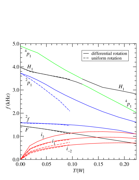
Figure 1: Frequencies of various modes for sequences A (solid lines) and AU (dashed lines). Note the avoided crossing between the $H_{1}$ and the ${}^{4}p_{1}$-mode.

In slowly rotating stars, the frequencies of all inertial modes increase linearly with increasing $T/|W|$ (see Friedman & Lockitch, 2001; Lockitch, Friedman & Andersson, 2003). At higher rotation rates, higher-order rotational terms can modify this behavior. For uniformly rotating stars, the expectation is that the inertial mode frequency still increases up to the mass-shedding limit. As clearly visible for the rapidly rotating models of sequence A in Fig. 1, this general expectation is no longer valid for differentially rotating stars (for a more detailed discussion, see Section 4.4).

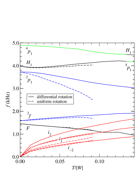
Figure 2: Same as Fig. 1, but for the sequences B and BU.

Due to differential rotation, the outer layers of the star rotate slower and the equatorial radius is smaller compared to a uniformly rotating model of same $T/|W|$. This leads to a smaller sound-crossing time and correspondingly higher fundamental mode frequencies for the differentially rotating models. This explains why the curves for the fundamental mode frequencies of the $F$ and ${}^{2\!}f$-mode of sequence A in Fig. 1 have smaller slopes than those corresponding to sequence AU. This behavior was already found for the same model sequence in the Cowling approximation in the work of SAF.

In general, higher order or large $l$ modes are affected more strongly by rotation than lower order or smaller $l$ modes. At large rotation rates this can lead to avoided crossings between mode sequences, where modes can exchange the character of their eigenfunctions. These avoided crossings are already known to exist from perturbative studies of axisymmetric modes in rotating Newtonian stars (Clement, 1986) and for relativistic quasi-radial modes (Yoshida & Eriguchi, 2001). It is not trivial to decide how to label the mode sequences after an avoided crossing. The decisive criterion for labeling a pulsation mode is not the continuity of the eigenfrequency along a mode sequence. More important is the character of the oscillation, i.e. the eigenfunction. One must therefore examine the eigenfunctions of two pulsations before and after an avoided crossing. Then the character of the modes after the crossing can be determined according to which modes (of those before the crossing) they resemble. Thus, continuity of eigenfunctions is preferred over continuity of eigenfrequencies in labeling modes.

4.2 Quasi-radial ($l=0$) modes and avoided crossings

The computed frequencies for the fundamental quasi-radial $l=0$ mode $F$ and its first overtone $H_{1}$ for the fixed rest mass sequences A and AU are displayed in Tables 2 and 3 and plotted in Fig. 1. Along the uniformly rotating sequence AU, there is a decrease in the frequency of the fundamental quasi-radial mode, since the central density of the star decreases with increasing rotation rate. For Newtonian nonrotating polytropic models the frequency of the fundamental quasi-radial mode is proportional to the square root of the average density. Even though we do not compute an average density for the rapidly rotating models of sequences A and AU, we notice that the decrease in the frequency of the $F$-mode from $1.458\mathrm{\ kHz}$ to $1.107\mathrm{\ kHz}$ along sequence AU follows closely the decrease in central energy density $\varepsilon_{\mathrm{c}}$. Along the differentially rotating sequence A, the frequency of the $F$-mode is further decreasing, reaching a very low value of $685\mathrm{\ Hz}$ for the most rapidly rotating model. Remarkably, when one compares models of same $T/|W|$ along the two sequences A and AU, the frequency of the $F$-mode is insensitive to the degree of differential rotation.

The first overtone $H_{1}$ also decreases along the uniformly rotating sequence AU, but by less than the near $\sqrt{\varepsilon_{\mathrm{c}}}$-dependence of the $F$-mode. Along the differentially rotating sequence A, the $H_{1}$-mode shows a similar insensitivity to the degree of differential rotation as the $F$-mode, when comparing models of same $T/|W|$, up to rotation rates of $T/|W|\sim 0.1$. For larger rotation rates, however, an extended avoided crossing with the ${}^{4}p_{1}$-mode takes place. Such avoided crossings exist, because the various mode sequences are affected to a different degree by rotation. In particular, the frequencies of higher $l$ modes tend to decrease faster with increasing $T/|W|$ than the frequencies of lower $l$ modes, leading to approaching mode-sequences. However, mode-sequences that contain similar terms in their eigenfunction expansions are not allowed to cross, even in the linear approximation (Clement, 1986; Yoshida & Eriguchi, 2001). Instead, two continuous sequences of pulsation frequencies avoid to cross, as shown in Fig. 1.

The character of the eigenfunctions along these continuous sequences is exchanged at an avoided crossing. As a result, the lower-frequency part of the continuous sequence starting as the $H_{1}$-mode in the nonrotating limit becomes the ${}^{4}p_{1}$-mode at large $T/|W|$. Correspondingly, the lower-frequency part of the continuous sequence which starts as the ${}^{4}p_{1}$-mode in the nonrotating limit, becomes the $H_{1}$-mode at large $T/|W|$. At the avoided crossing, the character of the eigenfunctions of both modes is a mixture of the eigenfunctions of the two modes before the avoided crossing. We have determined the correct labeling of the sequences after the avoided crossing by carefully comparing their two-dimensional eigenfunctions (see Section 5 for a discussion of how the eigenfunctions are obtained from our time-evolutions). The particular avoided crossing between the $H_{1}$ and ${}^{4}p_{1}$-modes was also observed along a sequence of rotating models in the relativistic Cowling approximation (Yoshida & Eriguchi, 2001).

Along the fixed central density sequences B and BU (see Tables 4 and 5 and Fig. 2), the frequency of the $F$-mode decreases, because, even though the central density stays fixed, rotational effects still increase the radius of the star, so that the sound crossing time in the equatorial region increases. This seems to have a monotonous influence on the frequency of the $F$-mode, which is again insensitive to the degree of differential rotation. The frequency of the $H_{1}$-overtone, on the other hand, first decreases somewhat with rotation, but then increases again, eventually surpassing its value of $3.971\mathrm{\ kHz}$ in the nonrotating limit. Since the $H_{1}$-mode has a node in its eigenfunction in the nonrotating limit, it is more sensitive to rotational effects (in comparison to the fundamental $F$-mode). These rotational effects have a different influence near the symmetry axis than near the equator. The changing dependence of the $H_{1}$-mode frequency as the star becomes more flattened reflects this sensitivity. In the case of sequence B, the avoided crossing between the $H_{1}$-mode and the ${}^{4}p_{1}$-mode happens at the largest rotation rates along this sequence. Consequently, the fastest rotating model B9 is in the avoided crossing region, where the mode eigenfunctions are mixed.

4.3 Quadrupole ($l=2$) modes

The computed frequencies for the fundamental quadrupole $l=2$ mode ${}^{2\!}f$ and its first overtone ${}^{2}p_{1}$ for the fixed rest mass sequences AU and A are displayed in Tables 3 and 2 and plotted in Fig. 1. Along the uniformly rotating sequence AU, there is only a small decrease in the frequency of the fundamental ${}^{2\!}f$-mode, from $1.586\mathrm{\ kHz}$ to $1.459\mathrm{\ kHz}$ at the mass-shedding limit. However, for the differentially rotating sequence A, the rate of decrease gets stronger for models with very high $T/|W|$, and the frequency of the fundamental ${}^{2\!}f$-mode becomes as small as $1.098\mathrm{\ kHz}$.

The first overtone ${}^{2}p_{1}$ shows a much stronger decrease in frequency with increasing rotation rates. Starting from $3.726\mathrm{\ kHz}$ at the nonrotating limit, along sequence AU its frequency becomes $2.090\mathrm{\ kHz}$ at mass-shedding, while it has a value of only $1.610\mathrm{\ kHz}$ for the fastest differentially rotating model along sequence A. A striking difference compared to all other modes studied here is that the frequency of the ${}^{2}p_{1}$-mode is indeed sensitive to the degree of differential rotation, as is evident from Figs. 1 and 2.

Along the fixed central density sequences B and BU the ${}^{2\!}f$-mode shows the opposite tendency compared to its behavior along the sequences A and AU, with its frequency increasing to $1.679\mathrm{\ kHz}$ and $1.917\mathrm{\ kHz}$, respectively (see Tables 4 and 5 and Fig. 2). In contrast, the frequency of the ${}^{2}p_{1}$-mode is still decreasing (although not as drastically as for sequences A and AU) with increasing rotation rates, reaching frequencies of $3.028\mathrm{\ kHz}$ at mass-shedding along sequence B and $2.483\mathrm{\ kHz}$ along sequence BU. The ${}^{2}p_{1}$-mode appears to be even more sensitive to the degree of differential rotation along the fixed central density sequence B than along the fixed rest mass sequence A.

4.4 Inertial modes

In our simulations we observe a large number of inertial modes, which are supported by the Coriolis force and become degenerate at zero frequency in nonrotating stars. From linear perturbation theory we expect that there exists an infinite number of inertial modes in a finite frequency range, which corresponds to 0 to $2\,\Omega$ for uniformly rotating Newtonian stars (see, e.g., Lockitch & Friedman, 1999). In spite of this, we do not find evidence for the excitation of an arbitrary number of inertial modes, but only a few specific inertial modes are predominantly excited. Since we do not make use of the eigenfunction recycling method to excite inertial modes (see Section 5), they are excited as by-products of the excitation of other modes. Hence, inertial modes can be excited either due to the non-exact nature of the initial trial eigenfunctions used to perturb the initial model (as described in Section 2.4) or due to non-linear couplings with linear polar modes (see discussion in Section 6.2). The fact that the amplitude of the observed inertial modes, with our choice of trial eigenfunctions, scales non-linearly with increasing amplitude, points to non-linear couplings as a possible origin, at least for most of the inertial modes we observe.

Examining the eigenfunctions of the excited inertial modes we notice that the mode with the usually highest PSD in a Fourier transform has only one node in the eigenfunction for $v_{\theta}$, while other modes at larger or smaller frequency than this ‘fundamental’ inertial mode have a larger number of nodes (increasing as the absolute frequency difference from the ‘fundamental’ inertial mode increases). Out of the many excited inertial modes, we choose to display in Tables 2 to 5 and Figs. 1 and 2 the ‘fundamental’ inertial mode with only one node in $v_{\theta}$, which we call $i_{1}$-mode, and the two modes with two nodes in the eigenfunction of $v_{\theta}$ on both sides of the $i_{1}$-mode in the frequency domain, which we denote the $i_{-2}$-mode and $i_{2}$-mode, respectively.

Figure 3: Comparison of the frequencies for the ${}^{2\!}f$ and ${}^{2}p_{1}$-mode (upper panel) and for the $F$ and $H_{1}$-mode (lower panel) in CFC (solid lines) and in the Cowling approximation (dashed lines) for the sequence of differentially rotating models A. In the lower panel we also show the frequencies of the ${}^{4}p_{1}$-mode after the avoided crossing with the $H_{1}$-mode (green line).

Notice that the number of nodes is determined at slow rotation rates and can change at very high rotation rates. Note also that inertial modes come in two flavours (polar-led and axial-led) and are hybrid modes in the sense that they do not reduce to either a pure polar or a pure axial mode in the nonrotating limit (see Lockitch & Friedman, 1999). A proper classification scheme for inertial modes, based on the dominant components in their eigenfunctions, is already in use (Lockitch & Friedman, 1999; Friedman & Lockitch, 2001; Lockitch, Friedman & Andersson, 2003). However, comparing our numerically calculated eigenfunctions with eigenfunctions obtained from linear perturbation theory with more simplifying assumptions (weak gravity or uniform density) is beyond the scope of the present paper and will be addressed in a separate publication. Thus, we use our own naming scheme for inertial modes simply for convenience, until proper identification is established in the future.

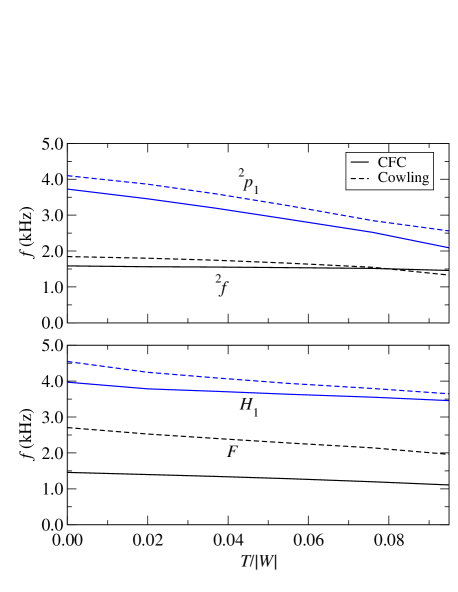
Figure 4: Same as Fig. 3, but for the sequence of uniformly rotating models AU.

Along sequence AU the frequencies of the three inertial modes increases monotonically with rotation. However, along sequence A the frequencies of the three inertial modes reach a maximum value for the rotation parameter $T/|W|$ being in the range 0.15 to 0.19, depending on the specific mode. This is due to the fact that, even though $T/|W|$ increases monotonically along sequence A, both the angular velocity at the centre and the angular velocity at the surface reach maximum values along this sequence, as can be seen in Table 1. On the other hand, along sequences BU and B the frequencies of the three inertial modes again increase monotonically, as does the angular velocity at the centre and at the surface.

4.5 Comparison to the Cowling approximation

When comparing the dependence of the mode frequency on $T/|W|$ plotted in Figs. 3 to 6 for the $F$, $H$, ${}^{2\!}f$, and ${}^{2}p_{1}$-modes obtained with the CFC approximation for the spacetime evolution against previous results in the Cowling approximation by SAF, several qualitative observations can be made. Apparently, for all sequences there is a large discrepancy in the values of the frequencies of the fundamental quasi-radial $F$-mode in the CFC simulations compared to the ones in the Cowling approximation at all rotation rates. This is also quantitatively evident in the relative differences of frequencies between the CFC and Cowling simulations of up to a factor $\sim 2$, listed for the nonrotating model (A0/AU0/B0/BU0) and the most rapidly rotating model of each sequence (A10, AU5, B9, BU9) in Table 7. We notice that these findings are consistent with those of Yoshida & Kojima (1997) for nonrotating stars. In terms of absolute differences, for the $F$-mode the Cowling approximation fails by far to predict the correct mode frequencies, as it yields values which are typically $\gtrsim 1\mathrm{\ kHz}$ too high. While in sequences A, AU, and BU the frequency curve in the Cowling approximation at least correctly captures the decline with increasing rotation rate, it cannot reproduce the similar behavior in sequence B.

We emphasize that neither in sequence A nor B we find any evidence for a splitting of the $F$-mode, a phenomenon that was noticed for those sequences in the Cowling approximation by SAF. This apparently confirms the possible explanation for the $F$-mode splitting as an artifact of the Cowling approximation offered in that work. In Figs. 3 to 6 and Table 7 we use the frequencies of the regular $F$-mode rather than those of the $F_{\mathrm{II}}$-mode of SAF, as the eigenfunctions of the latter mode do not possess the typical characteristics of a genuine $F$-mode (and, in addition, their amplitude of the frequency peak in FFTs is smaller than for the $F$-mode).

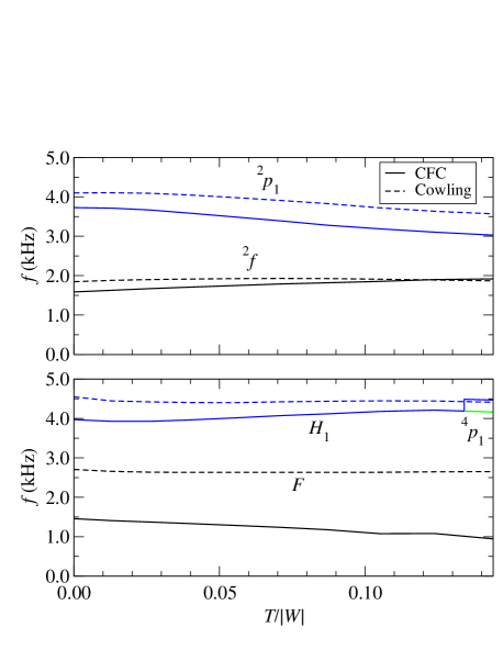
Figure 5: Same as Fig. 3, but for the sequence of differentially rotating models B.

Figs. 3 to 6 demonstrate that for the frequencies of the fundamental quadrupole ${}^{2\!}f$-mode and the $H_{1}$ and ${}^{2}p_{1}$-modes, the discrepancies between the CFC simulations and the Cowling approximation are much less severe (see also Table 7). In the case of the $H_{1}$-mode and the ${}^{2}p_{1}$-mode, the curve in the Cowling approximation follows our CFC results reasonably close, while we observe a crossing of the frequency curves for the ${}^{2\!}f$-mode beyond medium rotation rates in all sequences. Nevertheless, the ${}^{2\!}f$-mode frequencies still agree well quantitatively. Note however that avoided crossings of the $H_{1}$-mode and the ${}^{4}p_{1}$-mode (as in sequences A and B) complicates a comparison. If the continuous frequency curve of the $H_{1}$-mode is followed, the $H_{1}$-mode takes over the characteristics of the ${}^{4}p_{1}$-mode at the avoided crossing. Thus, if continuous frequency curves are compared, a possible change of the mode labeling must be taken into account. Although the simulations in the Cowling approximation reproduce the $H_{1}$, ${}^{2\!}f$, and ${}^{2}p_{1}$-mode frequencies from the CFC simulations fairly close for most sequences, which supports the idea of establishing empirical relations for predicting the correct frequencies from models evolved in the Cowling approximation, such relations should be used with caution (see discussion below).

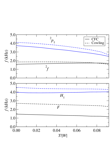
Figure 6: Same as Fig. 3, but for the sequence of uniformly rotating models BU.

Table 7: Relative difference in per cent in the frequencies of the $F$, $H_{1}$, ${}^{2\!}f$, and ${}^{2}p_{1}$-mode for the nonrotating model and the most rapidly rotating models of sequence A, AU, B, and BU in the Cowling approximation with respect to the CFC simulations. A $+$ sign ($-$ sign) indicates an overestimation (underestimation) of the CFC frequency in the Cowling approximation.

Model	$F$	$H_{1}$	${}^{2\!}f$	${}^{2}p_{1}$
A0/AU0/B0/BU0	$+86$	$+15$	$+16$	$+10$
A10	$+108$	$-12$	$-12$	$+18$
AU5	$+77$	$+5$	$-9$	$+22$
B9	$+81$	$-1$	$-3$	$+18$
BU9	$+98$	$+6$	$-7$	$+6$

For sequence BU a comparison of models evolved using a coupled evolution of hydrodynamics and spacetime, with no approximation for the gravitational field equations, against the Cowling approximation was presented by Font et al. (2002). Comparing these results with our new simulations using the CFC approximation as presented in Fig. 7 shows excellent agreement for the frequencies of the $F$-mode. This is another important confirmation of the validity of the results obtained with our code, considering in particular the differences in coordinate choice, grid resolution, evolution time, and assumption of CFC compared to the code employed in Font et al. (2002).

In the case of the $H_{1}$-mode we also find rather good agreement, with increasing mismatch as the models approach the mass-shedding limit. The oscillations in the $H_{1}$-mode frequency at large rotation rates observed in the fully relativistic simulations by Font et al. (2002) were interpreted as possible effects of avoided crossings. In contrast to this, in our simulations we find neither these oscillations nor signs of avoided crossing of the $H_{1}$-mode with other modes in sequences AU and BU (see Fig. 7, and also Figs. 1 and 2). For sequences A and B, where there is clear evidence for avoided crossing, this happens at larger rotation rates. We thus conclude that the oscillations visible in Fig. 7 (upper red dashed line) are an artifact which can be explained by the effectively lower grid resolution and shorter evolution time compared to the current simulations, as this increases the error in the numerical extraction of the mode frequency particularly for higher order modes.

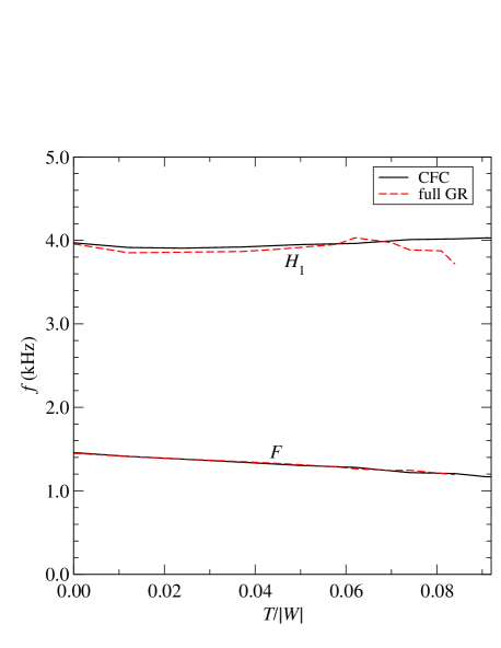
Figure 7: Comparison of the frequencies for the $F$ and $H_{1}$-mode in CFC (black solid lines) and full general relativity (red dashed lines) for sequence BU.

When comparing the frequencies for sequence BU from simulations with a dynamical spacetime to the ones in the Cowling approximation, Font et al. (2002) also observed that the frequencies for the $F$-mode (and, to a lesser degree, also the ones for the $H_{1}$-mode) show a similar dependence on the rotation rate in both cases. From the approximate constancy of the difference between the $F$-mode frequency and the corresponding result in the Cowling approximation, they constructed an approximate empirical relation for calculating the frequency of the $F$-mode for arbitrary rotation rates. This relation thus depends on the $F$-mode frequency of the nonrotating model BU0 obtained in a dynamical spacetime evolution and the variation of the $F$-mode frequencies with increasing rotation in the Cowling approximation. It yields the correct frequencies with an accuracy of better than 2 per cent for the most rapidly rotating in their model series of sequence BU (our model BU7).

Unfortunately our results clearly suggest that it is not possible to straightforwardly apply this simple method to set up analogous relations for sequences A, AU, and B, as shown in Figs. 3 to 6. Only for sequence BU, the $F$-mode frequency exhibits a nearly constant difference between the CFC and Cowling simulations irrespective of the rotation rate. Moreover, the frequencies of all other modes displayed in these figures also do not fulfill such a relation, except maybe in the case of the ${}^{2}p_{1}$-mode for sequences A and AU.

Lacking results from simulations involving evolution of the spacetime, SAF proposed an approximate relation for the $F$ and ${}^{2\!}f$-mode frequencies of sequence A similar to the one in Font et al. (2002). Based on the work by Yoshida & Kojima (1997) and Yoshida & Eriguchi (2001), an empirical relation was derived using information from the compactness of a model, and assuming nearly linear scaling of the frequencies with increasing rotation rate. When applying this relation to our model A10, we find a significant discrepancy between the predicted frequencies ($f_{F}=0.882\mathrm{\ kHz}$ and $f_{H_{1}}=0.757\mathrm{\ kHz}$) and the ones extracted from the actual numerical simulations ($f_{F}=0.685\mathrm{\ kHz}$ and $f_{H_{1}}=1.098\mathrm{\ kHz}$), with relative differences of 29 and 31 per cent for the $F$ and ${}^{2\!}f$-mode frequencies, respectively. Although their assumption of nearly linear scaling of $f_{F}$ and $f_{H_{1}}$ with the rotation rate is confirmed by our results (see Figs. 3 to 6), this error is much larger than the predicted uncertainty of the relation of a few per cent.

Owing to this, we refrain from establishing similar relations for other mode frequencies, even in cases where we also observe such nearly linear scaling of the frequency with rotation rate in CFC simulations and/or constant difference between the frequency of a specific mode in CFC and Cowling. We rather suggest that except in special cases, (the computationally expensive) simulations of rotating stars in which the spacetime and the hydrodynamics are coupled cannot be replaced by a combination of simulations in the Cowling approximation and simple empirical relations.

5 Eigenfunction recycling

As pointed out in Section 2.4, initial perturbations of the form given by Eqs. (11, 12) excite not only one desired specific eigenmode, but additional oscillation modes as well. This is clearly visible in the power spectrum of model A1 displayed in the upper panel of Fig. 8. While the fundamental modes $F$ and ${}^{2\!}f$ clearly dominate the spectrum, the overtones $H_{1}$ and ${}^{2}p_{1}$ along with several other modes are also significantly excited by a perturbation using the $l=0$ and $l=2$ trial eigenfunction of the initial velocity components $v_{r}$ and $v_{\theta}$, respectively.

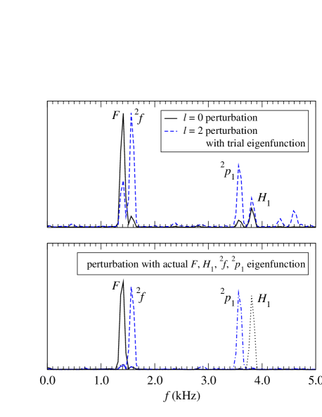
Figure 8: Fourier transform of the evolution of the radial profile of the rest-mass density $\rho$ along the equatorial plane for model A1. For the two simulations in the upper panel an $l=0$ and $l=2$ trial eigenfunction is used as perturbation, respectively, while the four recycling runs in the lower panel are excited with recycled eigenfunctions. The scaling of the ordinate is linear, and the power spectra in the upper panel are scaled to obtain the same strength of the $F$-mode.

This consequence of using trial eigenfunctions can be avoided by performing an additional ‘recycling’ run. For this the actual two-dimensional eigenfunctions of the $v_{r}$ and $v_{\theta}$ velocity components at a selected mode frequency are extracted from the original simulation which was perturbed by a trial eigenfunction. These eigenfunctions are then applied with appropriate amplitude as initial perturbation to a second simulation of the same stellar equilibrium model. In this case, other modes than the selected one are strongly suppressed, as shown for model A1 in the lower panel of Fig. 8. Here eigenfunctions of the $F$ and $H_{1}$-mode, and the ${}^{2\!}f$ and ${}^{2}p_{1}$-mode are extracted from a previous simulation perturbed with $l=0$ and $l=2$ trial eigenfunctions, respectively. These are then used as initial perturbations for four recycling runs with relative amplitudes with respect to the amplitude of the $F$ eigenfunction of 5.9, 3.8, and 7.0 for the $H_{1}$, ${}^{2\!}f$, and ${}^{2}p_{1}$ eigenfunction, respectively, in order to arrive at approximately equal strengths of the dominant modes in the power spectrum.

We note that the choice of using $v_{r}$ and $v_{\theta}$ eigenfunctions as initial perturbations for doing the recycling simulation is not arbitrary. Naively, one would think to use all four evolved variables $\rho$, $v_{r}$, $v_{\theta}$, and $v_{\varphi}$ instead. However, for a given mode some of these variables are out of phase with respect to the others. Using the eigenfunctions of all variables as recycling perturbations simultaneously without taking into account the relative phase between them does not lead to the excitation of a single mode, but to the excitation of a sum of different modes (similar to choosing a trial eigenfunction). From the phase information contained in the complex FFT of the various variables, we determined that, at least for the modes we are interested in, the quantities $v_{r}$ and $v_{\theta}$ have the same phase, while the other two are out of phase by $\pi/2$ with respect to $v_{r}$ and $v_{\theta}$.

While the suppression of undesired additional modes in the power spectrum significantly improves when eigenfunction recycling is performed, the form of the eigenfunction of various metric and hydrodynamic quantities extracted from the recycling run is usually altered only negligibly as compared to the eigenfunction extracted from the original simulation with the trial perturbation. In Fig. 9 we present radial profiles of the rest-mass density eigenfunction $\rho^{\mathrm{ef}}$ along the equatorial plane (upper panel) and of the $\theta$-velocity eigenfunction $v_{\theta}^{\mathrm{ef}}$ along $\theta=\pi/4$ (lower panel). They are extracted from both the original simulations of model A1 using $l=0$ (for $\rho^{\mathrm{ef}}$) and $l=2$ (for $v_{\theta}^{\mathrm{ef}}$) perturbations with trial eigenfunctions, and also from the respective $H_{1}$ and ${}^{2}p_{1}$ recycling runs. Only at the outer stellar boundary the shape of the eigenfunctions depends slightly on whether the model is perturbed by a trial or extracted eigenfunction, while in the bulk of the star the eigenfunctions are practically identical. We find similar results for the fundamental modes $F$ and ${}^{2\!}f$ and for the eigenfunctions of other metric and hydrodynamic quantities in model A1 and several other moderately rotating models.

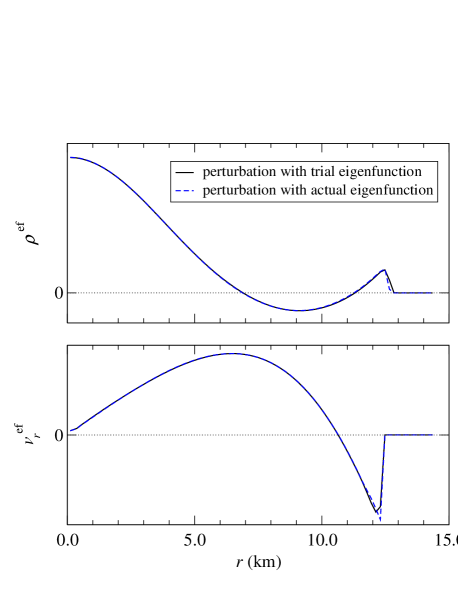
Figure 9: Radial profiles of the eigenfunctions $\rho^{\mathrm{ef}}$ for the $H_{1}$-mode (along the equatorial plane; upper panel) and $v_{\theta}^{\mathrm{ef}}$ for the ${}^{2}p_{1}$-mode (along $\theta=\pi/4$; lower panel) obtained from the evolution of model A1. For an initial perturbation using either a trial eigenfunction (black solid lines) or an extracted eigenfunction (blue dashed lines), the shapes of the eigenfunctions agree well. The eigenfunctions are scaled to the same maximum height.

We can thus conclude that for such rotating stellar models an initial perturbation with trial eigenfunctions is adequate to precisely obtain the mode frequency and to extract an accurate corresponding eigenfunction of the fundamental modes and their first overtones from the evolution. Additionally, for such models a single recycling run suffices to efficiently suppress the excitation of all unwanted modes. However, if the peak of the investigated mode in the power spectrum is small and/or if several modes interact (see also the discussion of avoided crossings in Section 4.2), which is typically the case for higher order modes in rapidly rotating models, another recycling loop may be necessary to clearly determine the mode frequency and eigenfunctions, and to channel most of the initial perturbation energy into a single oscillation mode.

Particularly in the case of the avoided crossing of the $H_{1}$ and the ${}^{4}p_{1}$-mode in sequence A and B (see also Figs. 1 and 2), we use a modified recycling strategy for an accurate mode analysis. Starting from a model where the mode frequency and eigenfunctions can still be clearly determined, the next model in the sequence is perturbed with the eigenfunctions of the investigated mode extracted from the previous model. This sequential recycling is a very helpful tool to resolve problems with ambiguous or unclear mode frequencies and character of the eigenfunction.

6 Non-linear pulsations

Although linear perturbations of rotating stars are assumed to have a vanishingly small amplitude, so that the background equilibrium star is unaffected by a linear oscillation mode, in certain situations non-linear effects can become important. Our non-linear evolution code allows us to investigate such effects, of which we present several cases in the following.

Figure 10: Fourier transform of the evolution of the radial profile of the rest-mass density $\rho$ along the equatorial plane for the nonrotating model (A0/AU0/B0/BU0) with an $l=0$ trial eigenfunction used as initial perturbation. Additional to linear modes, several non-linear harmonics can be identified.

6.1 Non-linear harmonics

The most basic non-linear effect we see in our simulations is the appearance of non-linear harmonics of the linear pulsation modes, a general property of non-linear systems (cf. Landau & Lifschitz, 1976, § 28). To lowest order, these arise as linear sums and differences of different linear modes, including self-couplings. If the system has eigenfrequencies $\omega_{i}$, the non-linearity of the equations excites modes at frequencies $\omega_{i}\pm\omega_{j}$, with amplitudes proportional to the product of the amplitudes of the combining frequencies. We note that such non-linear harmonics were also recently noticed by Zanotti et al. (2005) in the numerical investigation of the dynamics of oscillating, relativistic, high-density tori around Kerr black holes.

In Fig. 10 we present the Fourier PSD of the density evolution of the nonrotating model (A0/AU0/B0/BU0), to which a finite radial $l=0$ initial perturbation of the form (11) was added. In addition to the main linear modes $F$ and $H_{1}$, one can observe several of their non-linear harmonics, such as the self-couplings $2\cdot F$, $3\cdot F$ and the linear sums $H_{1}-F$ and $H_{1}-2\cdot F$. In the PSD a large number of additional peaks can be seen, and essentially all of those should correspond to non-linear harmonics of the excited linear modes. It is interesting to note that several non-linear harmonics are present that have frequencies much smaller than the fundamental radial mode $F$ (which, in the linear approximation, possesses the lowest frequency). These can actually fall into the frequency range of the inertial modes for rotating models. Thus, in rotating models further non-linear interactions between radial modes and inertial modes can be expected (see also the discussion in Section 6.2).

Non-linear harmonics can occur not only due to couplings between modes of the same index $l$ (such as the $l=0$ modes discussed above), but also due to couplings between modes of different $l$. Fig. 11 shows several identified harmonics that represent linear sums and differences between linear modes for the nonrotating model, when an $l=2$ perturbation was added to the initial data of the nonrotating model. Due to the approximate nature of the chosen trial eigenfunction, $l=0$ modes are also excited in addition to the main $l=2$ modes. The presence of both $l=0$ and $l=2$ modes then leads to the appearance of several non-linear harmonics, which include cases like ${}^{2}p_{1}-F$, $H_{1}-{}^{2\!}f$, etc. It is thus clear that even though in the linear approximation modes of different $l$ are orthogonal to each other (in a nonrotating perfect fluid star), non-linear effects couple all linear modes with different $l$ that are present in a non-linear simulation).

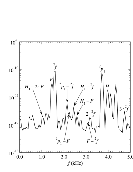
Figure 11: Same as Fig. 10, but with an $l=2$ trial eigenfunction used as initial perturbation.

In rotating models, where there can be a perplexing alternation of various linear modes and non-linear harmonics in a PSD plot, one can easily distinguish the non-linear harmonics from the linear modes by comparing PSDs produced from simulations with different initial perturbation amplitudes. As expected, the linear modes scale almost linearly, while the non-linear harmonics scale as the product of the amplitudes of the modes (or of the modes and harmonics) from which they are produced. Such a case is shown in Fig. 12, where model A1 from sequence A is used in which the linear modes $F$, $H_{1}$, ${}^{2\!}f$, and ${}^{2}p_{1}$ are all excited at roughly the same strength using the eigenfunction recycling technique for the initial perturbation as described in Section 5. Comparing two simulations of this model that differ by a common factor of 4 in the initial perturbation amplitude, one can clearly notice that while the amplitudes of the linear modes scale nearly linearly, the amplitudes of the various non-linear harmonics scale non-linearly (with many of them scaling roughly quadratically).

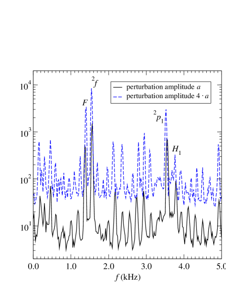
Figure 12: Fourier transform of the evolution of the radial profile of the $\theta$-velocity $v_{\theta}$ along $\theta=\pi/4$ for model A1 with a combined $F$, $H_{1}$, ${}^{2\!}f$, and ${}^{2}p_{1}$-mode eigenfunction as initial perturbation. Changing the perturbation amplitude $a$ reveals the non-linear scaling of the coupled modes as opposed to the linear scaling of the linear modes.

6.2 Non-linear 3-mode couplings

The presence of non-linear harmonics opens the possibility of 3-mode couplings when the star is rotating. The reason such 3-mode couplings can take place is the fact that the effect of rotation on the different modes varies. As was already discussed in Section 4.1, higher-order modes are typically affected stronger by rotation than lower-order modes, which results in avoided crossings between mode sequences. Rotation also influences the frequencies of the various non-linear harmonics to a different degree. Thus, at certain rotation rates, a non-linear harmonic can have the same frequency as a linear mode. Examples of such cases are demonstrated in Fig. 13, which shows the frequencies of several linear modes and of the two non-linear harmonics ${}^{2}p_{1}-{}^{2\!}f$ and $H_{1}-F$ as a function of $T/|W|$. Apparently the ${}^{2}p_{1}-{}^{2\!}f$ harmonic is crossing the frequency of the fundamental quasi-radial $F$-mode at about $T/|W|\sim 0.1$, while the $H_{1}-F$ harmonic is crossing the frequency of the ${}^{2}p_{1}$-mode at about $T/|W|\sim 0.12$. We also note that at any rotation rate one can expect several non-linear harmonics to coincide in frequency with some of the infinitely many inertial modes contained in the inertial mode range.

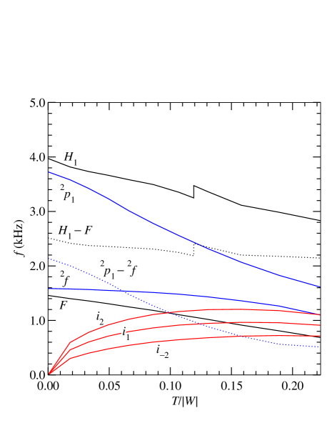
Figure 13: Frequencies of various linear modes and the two non-linear harmonics $H_{1}-F$ and ${}^{2}p_{1}-{}^{2\!}f$ for sequence A. At specific rotation rates the frequencies of linear and non-linear modes coincide, which can lead to non-linear 3-mode coupling.

At such crossings, the coinciding of the frequencies could potentially lead to resonance effects and even to parametric instabilities. In such a way, significant energy from one mode could be transfered to other modes. The most interesting case would be if pulsational energy from the quasi-radial mode, which weakly radiates gravitational waves, could be transfered non-linearly to stronger radiating nonradial modes. Since during core bounce a significant amount of kinetic energy is stored in the radial modes of pulsation, the transfer of even a small percentage of this kinetic energy to a nonradial mode could result in the emission of strong gravitational waves. This scenario has first been suggested by Clark (1979) and Eardley (1983), who investigated the parametric instabilities that could take place, using a Newtonian, slowly rotating collapse model (for recent related work for nonrotating or slowly rotating relativistic stars, see Passamonti et al., 2005).

In nonrotating or slowly rotating models, such a parametric instability can only take place under special conditions that would allow the two modes to be in resonance. Here we find that in rapidly rotating models rotational shifting of the frequency of different modes broadens the range of parameters for which interesting resonances could take place. We particularly notice that the quasi-radial mode will be in resonance with some inertial mode(s) for all rotation rates above a critical value. It is thus interesting to further study the possible energy transfer between different modes excited after, e.g., a core collapse or an accretion-induced collapse event, either on secular time-scales or as a parametric instability.

Here we only observe the necessary conditions for non-linear 3-mode couplings to take place. Whether such couplings will indeed lead to strong parametric resonances and enhanced gravitational wave emission remains to be investigated through much more detailed studies.

6.3 Mass-shedding-induced damping

Another striking example of a non-linear effect is the mass-shedding-induced damping of oscillations in stellar models which rotate at or near the mass-shedding limit. This new damping mechanism was first observed and discussed by SAF, and is especially important for pulsations in uniformly rotating stars. In SAF, the mass-shedding-induced damping was demonstrated for the uniformly rotating models BU8 and BU9 using fixed-spacetime evolutions, i.e. the Cowling approximation.

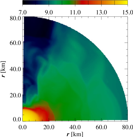
Figure 14: Distribution of the logarithm of the rest-mass density, $\log\rho$ ($\mathrm{g\ cm}^{-3}$), in the meridional plane for model BU9 with ideal fluid EOS at $t=4.4\mathrm{\ ms}$ in the Cowling approximation. The ordinate coincides with the rotation axis. The single shocks traveling through the atmosphere and creating a matter envelope are clearly visible. The black color coding corresponds to the low density artificial atmosphere where the rest-mass density is actually much smaller than $10^{7}\mathrm{\ g\ cm}^{-3}$. Note that only the innermost 80 km of the computational grid are shown.

As explained in SAF, the damping mechanism works as follows. As the star approaches the mass-shedding limit, the effective gravity near the equatorial surface diminishes, exactly vanishing at the mass-shedding limit. A small radial pulsation then suffices to cause mass-shedding after each oscillation period. As a result, a low-density envelope is created around the star. This envelope is initially concentrated in the regions close to the stellar equator, but with each oscillation period more and more mass is shed in the form of shock waves, and the envelope expands outwards and away from the equatorial plane. Since in rotating stars every pulsation mode also has a radial velocity component, the damping affects all modes. In SAF, it was found that the damping in the Cowling approximation can be rather strong. Here we investigate the same damping effect in the CFC approximation and compare the two cases.

We first repeat the study of the mass-shedding-induced damping for the radially perturbed model BU9, as presented in SAF, in the Cowling approximation. Fig. 14 shows the distribution of the rest-mass density $\rho$ in the meridional plane using the (nonisentropic) ideal fluid EOS (10). At time $t=4.4\mathrm{\ ms}$ several oscillations have already occurred and the high-entropy envelope has acquired a near-equilibrium state, extending into almost the entire computational grid (whose outer boundary has been set to 5 stellar equatorial radii with 120 additional logarithmically spaced radial grid points). Near the equatorial plane the envelope has a rest-mass density of $\sim 10^{-6}$ to $10^{-4}\rho_{\mathrm{c}}$, through which further consecutive shocks propagate. Only at angles $\lesssim 20^{\circ}$ (as measured from the rotation axis) does the high-entropy envelope not completely form.

We then study the same perturbed model (with a similar initial effective perturbation amplitude) but also evolving the spacetime, in the CFC approximation. Compared to the Cowling approximation, the mass-shedding behavior and the properties of the matter envelope are now significantly different. In Fig. 15, one can see (at the same time $t=4.4\mathrm{\ ms}$ as in Fig. 14) that the high-entropy envelope outside the star is confined to within roughly $45^{\circ}$ with respect to the equatorial plane, filled with matter of one to two orders of magnitude lower density than in the Cowling approximation. In addition, the consecutive shocks barely reach the outer grid boundary.

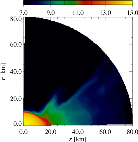
Figure 15: Same as Fig. 15, but for a spacetime coupled to the hydrodynamics (CFC simulation). Note that in contrast to the Cowling approximation, a much smaller angular part of the atmosphere is filled with a matter envelope, which also has significantly also lower density.

Fig. 16 shows the corresponding radial rest-mass density profiles along the equatorial plane for both the Cowling and CFC approximations. The envelope in the CFC approximation has a lower density than in the Cowling approximation, with the difference consistently increasing with distance and becoming 2 orders of magnitude at the outer grid boundary. In this plot the single shocks generated by the stellar oscillations, which first create the envelope and later propagate through it, are clearly noticeable. For model BU9 the frequency of the $F$-mode oscillations, which are mainly responsible for the mass-shedding in the above simulations is about twice as high in the Cowling than in the CFC approximation ($2.313\mathrm{\ kHz}$ vs. $1.169\mathrm{\ kHz}$). This is, however, not reflected in the shock pattern of the radial density profile in Fig. 16, where naively twice as many shocks between $r_{\mathrm{e}}$ and some radius $r>r_{\mathrm{e}}$ could be expected. This is a consequence of the unequal profiles of the shock propagation velocity in the envelope due to the different density profiles, as well as interactions of shocks traveling at different velocities due to unequal shock strengths. The latter effect can also lead to reverse shocks, which further complicate the picture. Note that in the density profile from the simulation in the Cowling approximation in Fig. 16, the significant loss of the matter in the stellar regions close to $r_{\mathrm{e}}$ by mass-shedding is evident, whereas in the CFC simulation the initial density profile inside the stellar boundary is nearly preserved.

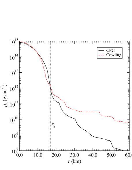
Figure 16: Radial profiles of the rest-mass density $\rho$ along the equatorial plane for model BU9 with ideal fluid EOS at $t=4.4\mathrm{\ ms}$ in CFC (black solid line) and in the Cowling approximation (red dashed line). The single shocks due to mass-shedding are clearly visible. The dotted line marks the equatorial stellar radius.

In an equilibrium model rotating at the mass-shedding limit, effective gravity at the equatorial surface vanishes due to a delicate balance between the pressure gradient, the gravitational force, and the centrifugal force. In the Cowling approximation the spacetime is held fixed during the entire simulation, and thus the gravitational force cannot react to local over- or underdensity caused by the pulsations. Evidently, in this case matter can easily be ejected from the stellar equatorial surface at each pulsation. In contrast to this, when the spacetime is coupled to matter it responds to changes in the hydrodynamic evolution. The most strongly excited pulsation mode in the mass-shedding simulations of model BU9 is the $F$-mode, whose rest-mass density eigenfunction $\rho^{\mathrm{ef}}$ features a node at $r_{\mathrm{n\,\rho}}\simeq 7\mathrm{\ km}$ in the equatorial plane, located at less than half the stellar equatorial radius (see Fig. 17). However, not everywhere in the star an over- or underdensity is reflected by an according localised increase or decrease of gravity, as the local gravitational pull is created by the global density distribution. Consequently, the nodes of the eigenfunctions of both the conformal factor $\phi^{\mathrm{ef}}$ and its negative radial derivative $-\partial_{r}\phi^{\mathrm{ef}}$ (representing the perturbation of the gravitational force) lie much farther out at $r_{\mathrm{n\,\partial_{r}\phi}}\simeq 14\mathrm{\ km}>r_{\mathrm{n\,\phi}}\simeq 11\mathrm{\ km}>r_{\mathrm{n\,\rho}}$. In a region $r_{\mathrm{n\,\rho}}<r\lesssim r_{\mathrm{n\,\phi}}$ the perturbations of density ($\rho^{\mathrm{ef}}$) and gravitational force ($\phi^{\mathrm{ef}}$, $-\partial_{r}\phi^{\mathrm{ef}}$) have opposite sign, and thus at some point during a pulsation cycle the gravitational force there decreases although the local density increases. Nevertheless, close to the stellar equatorial surface both $\phi^{\mathrm{ef}}$ and $-\partial_{r}\phi^{\mathrm{ef}}$ are again in phase with $\rho^{\mathrm{ef}}$, and remain greater than zero (albeit rather small) at the surface. Thus, whenever the local density there increases in a pulsation, this small local net gain in the gravitational pull suffices to efficiently attenuate mass-shedding, as observed in the CFC simulations.

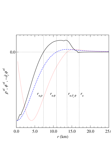
Figure 17: Radial profiles of the $F$-mode eigenfunction of the rest-mass density $\rho^{\mathrm{ef}}$ (black solid line), the conformal factor $\phi^{\mathrm{ef}}$ (blue dashed line), and its negative radial derivative $-\partial_{r}\phi^{\mathrm{ef}}$ (red dotted line) along the equatorial plane for model BU9 with ideal fluid EOS in CFC. The vertical dotted lines mark the locations $r_{\mathrm{n\,\rho}}$, $r_{\mathrm{n\,\phi}}$, $r_{\mathrm{n\,}\partial_{r}\phi}$ of the eigenfunction nodes and the equatorial stellar radius $r_{\mathrm{e}}$. The vertical scaling of the eigenfunctions is arbitrary, but their sign is not.

When matter is shed from the star, kinetic energy is carried away to the expense of the pulsational energy. Consequently, the pulsations of the star are gradually damped, depending on the intensity of mass-shedding. Fig. 18 shows the time evolution of the central rest-mass density for model BU9 obtained from the CFC simulation and the one in the Cowling approximation. It is evident that the damping of the pulsations is very strong in the latter case, leading to an approximate damping time-scale of $10\mathrm{\ ms}$. In contrast, the insignificant mass-shedding in the CFC simulation results in only small damping on a much longer time-scale. Actually, a long-term observation of the time evolution of $\rho_{\mathrm{c}}$ reveals that most of the decline of the oscillation amplitude in the time window of Fig. 18 can be explained by a mode-beating effect, which superimposes the genuine damping. Even with high initial perturbation amplitudes we are not able to observe significant unambiguous mass-shedding-induced damping during typical evolution times of $20\mathrm{\ ms}$. Simulations with lower initial perturbation amplitudes or of models which rotate not so close to the mass-shedding limit exhibit less mass-shedding compared to the above model, which is in accordance with the findings presented by SAF.

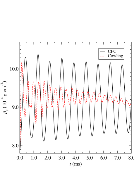
Figure 18: Time evolution of the central rest-mass density $\rho_{\mathrm{c}}$ for model BU9 with ideal fluid EOS at $t=4.4\mathrm{\ ms}$ in CFC (black solid line) and in the Cowling approximation (red dashed line). In the Cowling approximation, significant mass-shedding-induced damping can be seen, whereas the decline of the oscillation amplitude in CFC can be mostly attributed to mode-beating.

Even though in the CFC simulation the mass-shedding-induced damping of pulsations is not as strong as in the Cowling approximation, it could still have significant implications for unstable modes that grow on secular time-scales due to the gravitational-radiation driven CFS instability. In particular, the $l=m=2$ $f$-mode becomes unstable only near the mass-shedding limit in uniformly rotating stars (see Stergioulas & Friedman, 1998; Morsink, Stergioulas & Blattnig, 1999). A detailed investigation is required to determine whether the rate of mass-shedding-induced damping is shorter than the secular growth rate of the instability at amplitudes smaller than of order unity.

In Section 2.4 we have demonstrated that for exciting $F$-mode oscillations, an initial velocity perturbation of the form (11) is more appropriate than the density perturbation of Eq. (14) if the spacetime is coupled to the hydrodynamics. However, we have performed mass-shedding test simulations of model BU9 in the Cowling approximation, which show that in this case a velocity perturbation with typical amplitudes either results in a strong negative or positive drift in the time evolution of the central rest-mass density, depending on the sign of the initial perturbation amplitude. Avoiding this by significantly reducing the initial perturbation amplitude in turn effectively suppresses the mass-shedding and the resulting damping of the stellar pulsations. Following SAF, we therefore use the density perturbation (14) for the simulations of the mass-shedding model BU9 in both CFC and the Cowling approximation presented here. To compensate for the amplification of the oscillation amplitude during evolution using equal initial perturbation amplitudes for a coupled spacetime as compared to the Cowling approximation (see Section 2.4), we use different initial perturbation amplitudes in CFC ($a=0.01$) than in the Cowling approximation ($a=0.05$). This yields an approximately equal height of the first oscillation peak during the evolution (see Fig. 18), so that we can consider the initial conditions in the two simulations to be similar.

7 Gravitational waves

In the numerical simulations of the models presented above, we extract the gravitational waves emitted by the pulsations initiated in each model. For this we use the Newtonian quadrupole formula in its time-integrated form (as described in detail in Dimmelmeier, Font & Müller, 2002b), which yields the quadrupole wave amplitude $A^{\mathrm{E2}}_{20}$ as the lowest order term in a multipole expansion of the radiation field into pure-spin tensor harmonics (Thorne, 1980).

7.1 Gravitational wave power spectrum

Fig. 19 shows the gravitational wave power spectrum (i.e. the PSD of the time evolution of $A^{\mathrm{E2}}_{20}$) for a series of simulations of model A1 (i.e. the most slowly rotating model of sequence A) in which the $F$, $H_{1}$, ${}^{2\!}f$, and ${}^{2}p_{1}$-modes are individually excited using the eigenfunction recycling technique. As already stated in Section 5 the initial excitation amplitude $a$ for each individual mode was chosen such that the PSDs of the integrated density variations in the equatorial plane reach similar amplitudes (see also lower panel of Fig. 8). However, this choice for $a$ results in a different relative oscillation amplitude $\delta\rho_{\mathrm{c}}$ of the central density during the evolution (with $2\delta\rho_{\mathrm{c}}$ being the density variation measured top to bottom of the oscillation) for each of the four simulations. In Fig. 19 we thus scale the original gravitational wave signal such that it corresponds to $\delta\rho_{\mathrm{c}}=1\mathrm{\ per\ cent}$. This is possible as we find that the maximum amplitude $|A^{\mathrm{E2}}_{20}|_{\mathrm{max}}$ of the quadrupole signal is approximately proportional to $\delta\rho_{\mathrm{c}}$ (and in turn also to $a$) to fair accuracy for the four linear stellar pulsation modes investigated here.

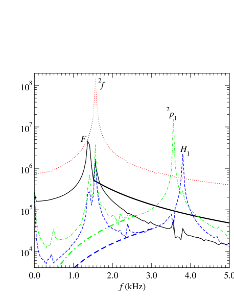
Figure 19: Gravitational wave power spectrum for model A1 excited with recycled eigenfunctions of the $F$, $H_{1}$, ${}^{2\!}f$, and ${}^{2}p_{1}$-mode, respectively. In the $F$, $H_{1}$, and ${}^{2}p_{1}$-mode recycling runs a significant ${}^{2\!}f$-mode component is also present in the gravitational wave signal. The thick lines indicate an artifical fall-off with quadratic frequency dependence assumed to get rid of these spurious contributions. Units on the $y$-axis are arbitrary.

As expected, the quadrupolar ${}^{2\!}f$-mode is the strongest emitter of gravitational waves, while the other three modes are still within roughly one or two orders of magnitude of this dominant gravitational wave emitting mode. Note that an excitation of the ${}^{2\!}f$-mode results in a nearly monochromatic gravitational wave power spectrum, indicating that the recycled eigenfunctions used for exciting this mode are of high accuracy. The PSD for the individual excitations of the $F$, $H_{1}$, and ${}^{2}p_{1}$-mode are also dominated by the appropriate frequency of the respective mode, but exhibit also additional contributions of other excited modes. These contributions are usually small (at least one order of magnitude smaller than the dominant mode), but as the quadrupole ${}^{2\!}f$-mode strongly radiates gravitational waves, a small leaking of energy into that mode from the main excitation mode is sufficient to exhibit a significant contribution at that specific frequency. This is particularly apparent in the case of the $H_{1}$-mode, which radiates gravitational waves only through its rotationally-induced $l\geq 2$ terms.

In order to suppress the unwanted ${}^{2\!}f$-mode contribution in the computation of the characteristic signal frequency and amplitude in the following Section 7.2, for the gravitational wave power spectrum of the $F$, $H_{1}$, and ${}^{2}p_{1}$-mode simulations we have assumed a fall-off behavior with quadratic frequency dependence in the region of the spectrum where the spurious ${}^{2\!}f$-mode is located (indicated by thick lines in Fig. 19).

We also note that for the excitations of the overtones $H_{1}$ and ${}^{2}p_{1}$ with recycled eigenfunction, some inertial modes (visible at the low-frequency end in the PSD of Fig. 19) also weakly contribute to the emission of gravitational waves.

7.2 Detectability of gravitational waves

In order to assess the prospects for detectability of the gravitational wave signal from our models of pulsating neutron stars by current and planned interferometer detectors, we calculate the characteristic dimensionless amplitude $h_{\mathrm{c}}$ of the signal from the quadrupole wave amplitude $A^{\mathrm{E2}}_{20}$ as described in Zanotti et al. (2005). We perform a Fourier transform of the transverse traceless gravitational wave signal,

$$\tilde{h}(f)=\int_{-\infty}^{\infty}\!\!e^{2\pi ift}h^{\mathrm{TT}}(t)\,dt,$$ (15)

where

$$h^{\mathrm{TT}}=\frac{1}{8}\sqrt{\frac{15}{\pi}}\frac{A^{\mathrm{E2}}_{20}}{r_{\mathrm{gw}}}$$ (16)

in the equatorial plane of the neutron star (assuming optimal detection geometry of the interferometer) with $r_{\mathrm{gw}}$ being the distance from the emitting source to the detector. To obtain the detector dependent characteristic signal frequency

$$f_{\mathrm{c}}=\left(\int_{0}^{\infty}\!\frac{\langle|\tilde{h}|^{2}\rangle}{S_{h}}f\,df\right)\left(\int_{0}^{\infty}\!\frac{\langle|\tilde{h}|^{2}\rangle}{S_{h}}df\right)^{-1}$$ (17)

and characteristic signal amplitude

$$h_{\mathrm{c}}=\left(3\int_{0}^{\infty}\!\frac{S_{h\mathrm{\,c}}}{S_{h}}\langle|\tilde{h}|^{2}\rangle f\,df\right)^{1/2}\!\!\!\!\!\!\!\!,$$ (18)

the power spectral density $S_{h}$ of the detector is needed (with $S_{h\mathrm{\,c}}=S_{h}(f_{\mathrm{c}})$). We approximate the average $\langle|\tilde{h}|^{2}\rangle$ over randomly distributed angles by $|\tilde{h}|^{2}$. From Eqs. (17, 18) the signal-to-noise ratio can be computed as $S/N=h_{\mathrm{c}}/[h_{\mathrm{rms}}(f_{\mathrm{c}})]$, where $h_{\mathrm{rms}}(f_{\mathrm{c}})=\sqrt{f_{\mathrm{c}}S_{h}(f_{\mathrm{c}})}$ is the value of the rms strain noise (i.e. the theoretical sensitivity window) for the detector at the characteristic frequency.

In Table 8 we give the values of $f_{\mathrm{c}}$ and $h_{\mathrm{c}}$ for the gravitational wave signal emitted by the most slowly rotating model A1 excited with recycled eigenfunctions, computed for the theoretical power spectral density $S_{h}$ of the detectors VIRGO, LIGO I and advanced LIGO located at a distance of $r_{\mathrm{gw}}=10\mathrm{\ kpc}$ from the source. The strong emission of the gravitational waves by the quadrupolar ${}^{2\!}f$-mode and its first overtone ${}^{2}p_{1}$ is reflected by the large wave amplitudes $h_{\mathrm{c}}$ of $\sim 400\times 10^{-22}$ and $\sim 80\times 10^{-22}$, respectively, compared to only $\sim 20\times 10^{-22}$ for the $F$-mode and $\sim 10\times 10^{-22}$ for the $H_{1}$-mode.

Table 8: Characteristic frequency $f_{\mathrm{c}}$ and characteristic amplitude $h_{\mathrm{c}}$ for a gravitational wave signal emitted by the most slowly rotating model A1 excited with recycled eigenfunctions of the $F$, $H_{1}$, ${}^{2\!}f$, and ${}^{2}p_{1}$-mode, respectively, as prospectively seen by various interferometer detectors. For comparison, the frequency $f$ of the respective stellar oscillation mode is also given. All frequencies are in kHz, and $h_{\mathrm{c}}$ is given in units of $10^{-22}$ for a source at $r_{\mathrm{gw}}=10\mathrm{\ kpc}$ oscillating with $\delta\rho_{\mathrm{c}}=1\mathrm{\ per\ cent}$. The signal duration time is assumed to be $t_{\mathrm{gw}}=20\mathrm{\ ms}$.

		VIRGO		LIGO I		adv. LIGO
Mode	$f$	$f_{\mathrm{c}}$	$h_{\mathrm{c}}$	$f_{\mathrm{c}}$	$h_{\mathrm{c}}$	$f_{\mathrm{c}}$	$h_{\mathrm{c}}$
$F$	1.400	1.370	19.3	1.338	18.9	1.236	17.4
$H_{1}$	3.816	3.783	12.1	3.792	12.1	3.791	12.1
${}^{2\!}f$	1.577	1.524	463.3	1.467	467.5	1.292	393.8
${}^{2}p_{1}$	3.580	3.545	76.9	3.545	76.9	3.544	76.9

Note that we integrate $h^{\mathrm{TT}}$ over a finite duration time of $t_{\mathrm{gw}}=20\mathrm{\ ms}$ in the FFT and scale $\delta\rho_{\mathrm{c}}$ to 1 per cent for each individual excited mode. To compute $h_{\mathrm{c}}$ in a straightforward way from the values given in Table 8 for an arbitrary source distance, signal duration, and central oscillation amplitude of the star, the following simple scaling laws can be used: $h_{\mathrm{c}}\propto r_{\mathrm{gw}}^{-1}$ and $h_{\mathrm{c}}\propto\sqrt{t_{\mathrm{gw}}}$, while $h_{\mathrm{c}}\propto|A^{\mathrm{E2}}_{20}|_{\mathrm{max}}$ for a given power spectral density $S_{h}$ and thus approximately proportional to $\delta\rho_{\mathrm{c}}$ (see discussion in Section 7.1).

As we artificially remove the spurious contribution of the quadrupole ${}^{2\!}f$-mode to the gravitational wave power spectrum of the $F$, $H_{1}$, and ${}^{2}p_{1}$-mode recycling runs (see Section 7.1), the small discrepancy between the values for characteristic gravitational wave signal frequency $f_{\mathrm{c}}$ and the stellar oscillation mode frequency $f$ in Table 8 is predominantly caused by the dependence of $f_{\mathrm{c}}$ on the power spectral density $S_{h}$ of the specific detector. Accordingly, as $h_{\mathrm{c}}\neq h^{\mathrm{TT}}$, the values of characteristic amplitudes $h_{\mathrm{c}}$ are slightly different for each detector. The effect of $S_{h}$ on $f_{\mathrm{c}}$ and $h_{\mathrm{c}}$ is strongest for the gravitational wave signal emitted by the relatively low frequency modes $F$ and ${}^{2\!}f$.

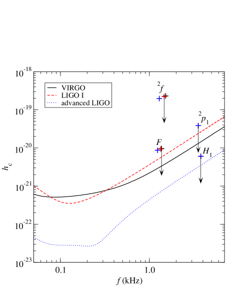
Figure 20: Distribution of the characteristic gravitational wave signal amplitude $h_{\mathrm{c}}$ in the frequency space for model A1 excited with recycled eigenfunctions of the $F$, $H_{1}$, ${}^{2\!}f$, and ${}^{2}p_{1}$-mode, respectively. The crosses represent $h_{\mathrm{c}}$ for a source at $r_{\mathrm{gw}}=10\mathrm{\ kpc}$, oscillating with $\delta\rho_{\mathrm{c}}=5\mathrm{\ per\ cent}$. The signal duration time is assumed to be $t_{\mathrm{gw}}=20\mathrm{\ ms}$. The sensitivities $h_{\mathrm{rms}}$ of the interferometer detectors VIRGO (black solid line), LIGO I (red dashed line), and advanced LIGO (blue dotted line) are also shown. Particularly for the $F$ and ${}^{2\!}f$-mode signal, the value of $h_{\mathrm{c}}$ and $f_{\mathrm{c}}$ is slightly dependent on the sensitivity of the respective interferometer detector, as indicated by the color coding. The arrows indicate the location of $h_{\mathrm{c}}$ for $\delta\rho_{\mathrm{c}}=1\mathrm{\ per\ cent}$.

In Fig. 20 we show the location of the characteristic gravitational wave amplitude $h_{\mathrm{c}}$ for the $F$, $H_{1}$, ${}^{2\!}f$, and ${}^{2}p_{1}$-mode signal of model A1 in relation to the sensitivity windows of VIRGO, LIGO I, and advanced LIGO. We again assume a distance to the source of $r_{\mathrm{gw}}=10\mathrm{\ kpc}$, i.e. within our Galaxy, and (in contrast to Table 8) an oscillation amplitude $\delta\rho_{\mathrm{c}}=5\mathrm{\ per\ cent}$. In such a scenario the gravitational wave signal from a neutron star pulsating in the ${}^{2\!}f$-mode with the adopted oscillation amplitude would be clearly detectable even by current interferometer observatories with a signal-to-noise ratio of around 50 for VIRGO and LIGO I (and 300 for the planned advanced LIGO detector). On the other hand, the $F$ and ${}^{2}p_{1}$-mode signals lie only marginally above the sensitivity threshold of current detectors, corresponding to a signal-to-noise ratio of at most $\sim 2$. The wave signal from the $H_{1}$-mode, in turn, could possibly be detectable only by the proposed advanced LIGO detector for the selected pulsation amplitude and duration.

If $\delta\rho_{\mathrm{c}}$ is reduced to 1 per cent, as exemplified by the arrows in Fig. 20, the $F$ and ${}^{2}p_{1}$-mode signals clearly fall out of the sensitivity window of VIRGO and LIGO I, but would be detectable by advanced LIGO, while the $H_{1}$-mode signal is now evidently out of the range even for the latter. Only the signal from the ${}^{2\!}f$-mode still exhibits a signal-to-noise ratio of around 10 for the current detectors. It is important to note that using the scaling properties of the signal discussed above, the data presented in Fig. 20 can be used to determine the necessary minimum stellar oscillation amplitude $\delta\rho_{\mathrm{c}}$, maximum source distance $r_{\mathrm{gw}}$, and minimum signal duration time $t_{\mathrm{gw}}$ required for a prospective detection (set by a specific signal-to-noise ratio above 1) of the gravitational wave emitted by model A1.

We also emphasize that the frequencies of the investigated linear pulsation modes $F$, $H_{1}$, ${}^{2\!}f$, and ${}^{2}p_{1}$ are located at the rapidly ascending high frequency slope of the detector sensitivity curves. Consequently, for the fixed rest mass sequences A and AU the decrease of the frequencies for these modes with increasing rotation can enhance the prospects for detection by shifting the signals towards the more sensitive domain of the detector sensitivity window. For the fixed central density sequences B and BU, however, the opposite dependence of the $H_{1}$ and particularly of the ${}^{2\!}f$-mode frequencies on rotation reverses this effect for these two modes.

Further increase of the signal-to-noise ratio of the gravitational wave signals presented here could be achieved with the advanced LIGO detector, using its planned ability to be tuned at higher frequencies in a narrow-banding mode. The chances for a successful detection of neutron star oscillation modes will also rise dramatically by the simultaneous operation of high-frequency-band detectors such as the proposed dual sphere detectors (Cerdonio et al., 2001), which are designed to have an improved sensitivity at frequencies of a few kHz and would thus be particularly suitable for detecting the first overtones $H_{1}$ and ${}^{2}p_{1}$.

7.3 Gravitational wave asteroseismology

It is clear from the discussion of our results so far, that pulsating rotating neutron stars are gravitational wave sources that depend on several parameters (EOS, mass, angular momentum, differential rotation law, initial perturbation amplitude, damping mechanisms, etc.). All these parameters may have different effects on the oscillation spectrum of the star and, therefore, the successful extraction of the physical characteristics of the source from the gravitational wave signal will be difficult to achieve. It is important to isolate each effect on the gravitational waveform in order to find general trends.

Empirical formulas that can be used for gravitational wave asteroseismology (with the aim of pin-pointing the correct high-density EOS through gravitational wave observations) were constructed in recent years (Andersson & Kokkotas, 1998; Kokkotas, Apostolatos & Andersson, 2001; Benhar, Ferrari & Gualtieri, 2004), assuming nonrotating cold equilibrium models. Thus, these formulas contain only the effect of EOS and mass. More recently, finite temperature effects and slow-rotation effects on the mode frequencies were computed (Ferrari, Miniutti & Pons, 2003a, b; Ferrari et al., 2004), but these effects have not yet been incorporated in the empirical formulas for asteroseismology. In our work we focus on the effects of rotation, using a particular cold EOS as an example. A complete treatment will, of course, require using a large sample of realistic EOSs, but such an attempt is beyond the scope of this work. Using only the frequencies extracted from the simulations presented here, we can nevertheless identify several interesting features that indicate qualitatively the influence of rotation on the empirical formulas used in gravitational wave asteroseismology.

First, the frequencies of most modes show a simple dependence on rotation so that the empirical formulas obtained for nonrotating stars could be extended to rotation by multiplying with a factor containing only one or two powers of a rotational parameter such as $T/|W|$. The exception is the $H_{1}$-mode, which will require special treatment due to the avoided crossing at moderate values of $T/|W|$. Second, the frequencies of most modes, such as the $F$, ${}^{2\!}f$ and $H_{1}$-mode, become nearly independent of the degree of differential rotation when parametrized as a function of $T/|W|$. However, the frequency of the ${}^{2}p_{1}$-mode is strongly affected by the degree of differential rotation. Thus, an additional parameter, measuring the strength of differential rotation, could be built into an empirical formula for this specific mode.

Ideally, if the four modes $F$, $H_{1}$, ${}^{2\!}f$, and ${}^{2}p_{1}$ were detected, then a set of empirical formulas for their frequencies, constructed in the way described above, would allow the simultaneous extraction of the mass, radius, $T/|W|$, and degree of differential rotation. Of course, this ideal situation may become more complicated by the inclusion of finite temperature effects, which would add at least one more parameter to the system.

8 Summary and Outlook

Using the axisymmetric general relativistic hydrodynamics code CoCoNuT we have investigated pulsations of uniformly and differentially rotating neutron star models. We have compared our numerical simulations, in which the spacetime dynamics is coupled to the evolution of the fluid, to previous results performed under the assumption of a fixed spacetime (Cowling approximation). In the present work we have used the so-called conformal flatness condition (CFC) for the spatial three-metric, this being an excellent and well-tested approximation of the exact spacetime in the regime studied here. The coupled system of (hyperbolic) hydrodynamics and (elliptic) metric equations has been solved using the novel approach of combining Riemann-solver-based HSRC methods for the fluid evolution and spectral methods for the computation of the spacetime metric (Dimmelmeier et al., 2005).

As equilibrium initial data we have constructed four sequences of relativistic polytropes with parametrized rotation, which have then been perturbed by small amplitude $l=0$, 2, or 4 trial eigenfunctions to excite pulsation modes. By analyzing the time evolutions of various hydrodynamic and metric quantities using Fourier transforms along radial profiles or on the entire spatial grid, we have obtained the pulsation frequencies for the fundamental quasi-radial ($l=0$) $F$-mode, the fundamental quadrupole ($l=2$) ${}^{2\!}f$-mode, and their respective overtones, the $H_{1}$ and ${}^{2}p_{1}$-mode, as well as three inertial modes labelled $i_{-2}$, $i_{1}$, and $i_{2}$. Additionally, for two differentially rotating sequences we have obtained the frequencies for the ${}^{4}f$ and ${}^{4}p_{1}$-mode. We have found that for these two sequences the ${}^{4}p_{1}$-mode engages in an avoided crossing with the $H_{1}$-mode. This is a consequence of the different influence of rotation on the frequency of these two modes, which brings their frequencies closer with increasing rotation rate. At the avoided crossing, an exchange of the character of eigenfunctions of the $H_{1}$ and ${}^{4}p_{1}$-mode has been observed. Although linear perturbation theory predicts the existence of an infinite number of inertial modes in a finite frequency range, in our simulations we have detected the predominant excitation of only a few specific inertial modes, which are excited as by-products of the excitation of other modes. For the differentially rotating sequence of fixed rest mass, the inertial mode frequencies reach a maximum value before the mass-shedding limit is reached and then decrease again.

In order to suppress the simultaneous excitation of more than one mode, which is typically the case when trial eigenfunctions are used as initial perturbations, we have employed a new technique, which we call eigenfunction recycling. For this, we first extract the two-dimensional eigenfunction of velocity components at the frequency of the mode under consideration and then apply it as an initial perturbation in a second simulation of the original neutron star model. This selective excitation of modes works very well even for overtones.

When comparing the frequency curves of the $F$-mode for all four investigated sequences with previous results in the Cowling approximation, we have observed that the latter typically overestimate the correct frequency by about a factor of 2 (corresponding to an absolute difference of $\sim 1\mathrm{\ kHz}$), which is consistent with similar findings for nonrotating stars by Yoshida & Kojima (1997). Moreover, we have found no evidence for the $F$-mode splitting found by SAF to occur in the Cowling approximation. Thus, we conclude that this effect is an artifact which can be attributed to the Cowling approximation, as was suggested in SAF. On the other hand, for the $H$, ${}^{2\!}f$, and ${}^{2}p_{1}$-mode frequencies, much closer agreement with the Cowling results of SAF has been found. For these modes the relative difference is usually less than $\sim 20\mathrm{\ per\ cent}$. Concerning empirical formulas constructed by Font et al. (2002) and SAF using results in the Cowling approximation in order to predict mode frequencies for rotating sequencies, we have found that the changing characteristics of equilibrium models along various sequences significantly affect the relative differences between the actual frequencies and those obtained in the Cowling approximation. As a result, such empirical relations can only be of limited validity, while still representing a significant improvement compared to the Cowling approximation.

Even though we have used only small-amplitude initial perturbations, the use of a non-linear evolution code has allowed us to investigate various non-linear effects in pulsating neutron star models. We have observed non-linear harmonics of the linear pulsation modes of our stellar models, arising as linear sums and differences of various linear modes, including self-couplings (for similar findings in high-density accretion tori around Kerr black holes, see Zanotti et al., 2005). For rotating models such non-linear harmonics actually fall into the frequency range of the inertial modes and could interact with linear modes in non-linear 3-mode couplings in the form of a resonance or a parametric instability. It would be interesting to investigate under which conditions strong mode couplings or instabilities can occur.

In SAF a new non-linear damping mechanism for non-linear pulsations was found to operate in uniformly rotating models that are near the mass shedding limit. The damping of pulsations is due to mass shedding, when fluid elements near the equator become unbound due to the radial component of the velocity perturbation. This mass-shedding-induced damping could have severe consequences for, e.g., the $f$-mode gravitational-wave driven CFS instability, which grows on a secular time-scale. Here we have found that while the actual mass-shedding-induced damping does not occur on dynamical time-scales (as in the Cowling approximation) it is still present on secular time-scales, so that a detailed comparison to the $f$-mode growth rate is required in order to determine the outcome of the $f$-mode instability.

Taking into account that in the core collapse simulations by Dimmelmeier, Font & Müller (2001, 2002a, 2002b) the dominant quadrupole contribution had an effective gravitational wave amplitude that was roughly one to two orders of magnitude above the sensitivity curve of the advanced LIGO detector, it is likely that in a favourable detection event several pulsation modes of the proto-neutron star may be detected simultaneously. We have thus investigated the gravitational wave signals (in the Newtonian quadrupole approximation) emitted by the linear modes $F$, $H_{1}$, ${}^{2\!}f$, and ${}^{2}p_{1}$, for a slowly rotating neutron star model. In order to estimate the prospects for detectability of the signal by interferometric detectors, we have computed the (weakly detector dependent) characteristic signal frequency and amplitude for the theoretical power spectral density of VIRGO, LIGO I, and advanced LIGO. We infer that for a pulsation amplitude of the stellar central density of 5 per cent a gravitational wave signal from the investigated modes (with the exception of the $H_{1}$-mode) is measurable by current detectors, if the signal is integrated over a time of at least $20\mathrm{\ ms}$ and the source is located in our Galaxy. We have shown how scaling properties of the signal can be used to determine the necessary minimum stellar pulsation amplitude, maximum source distance, and minimum signal duration time required for a prospective detection. We have also discussed how effects of rotation can qualitatively influence empirical formulas used in gravitational wave asteroseismology and can thus help to constrain parameters of neutron star models in the case of a successful detection of gravitational waves from pulsation modes. A more complete study of the detectability of various modes for all equilibrium models of our sequences will appear elsewhere.

In the relativistic core collapse simulations by Dimmelmeier, Font & Müller (2001, 2002a, 2002b) the quasi-periodic gravitational waves emitted around core bounce were found to have frequencies less than roughly $1.1\mathrm{\ kHz}$. On the other hand, for nonrotating models constructed with a large sample of different realistic EOSs, the frequencies of the fundamental $l=2$ quadrupole $f$-mode range from $\sim 1.35\mathrm{\ kHz}$ for extremely stiff EOSs to $\sim 3.6\mathrm{\ kHz}$ for extremely soft EOSs (see, e.g., Andersson & Kokkotas, 1998). One of the main effects lowering the frequency of emitted gravitational waves is rotation. In our differentially rotating sequence of fixed rest mass, the nonrotating model has a fundamental $l=2$ $f$-mode frequency of $\sim 1.6\mathrm{\ kHz}$, which decreases to $\sim 1.1\mathrm{\ kHz}$ at the largest rotation rate. Therefore, additional effects must be taken into account in order to explain the wider range of frequencies found by Dimmelmeier, Font & Müller (2001, 2002b). One such important factor is the high entropy in a proto-neutron star immediately after core bounce. The proto-neutron star is surrounded by a hot envelope into which the pulsations of the interior can penetrate, increasing the period of each pulsation (see Ferrari, Miniutti & Pons, 2003a). Thus, a natural extension of our investigation will be to compute the frequencies of the various axisymmetric modes for a realistic proto-neutron star structure.

References

- Alcubierre et al. (2004) Alcubierre M. et al., 2004, Class. Quantum Grav., 21, 589
- Andersson & Kokkotas (1998) Andersson N., Kokkotas K. D., 1998, MNRAS, 299, 1059
- Arnowitt, Deser & Misner (1962) Arnowitt R., Deser S., Misner C. W., 1962, in Witten L., ed, Gravitation: An introduction to current research. Wiley, New York b
- Banyuls et al. (1997) Banyuls F., Font J. A., Ibáñez J. M., Martí J. M., Miralles J. A., 1997, ApJ, 476, 221
- Benhar, Ferrari & Gualtieri (2004) Benhar O., Ferrari V., Gualtieri L., 2004, Phys. Rev. D, 70, 124015
- Bernuzzi & De Pietri (2006) Bernuzzi, S., De Pietri, R., 2006, private communication
- Bonazzola et al. (2004) Bonazzola S., Gourgoulhon S., Grandclément P., Novak J., 2004, Phys. Rev. D, 70, 104007
- Cerdá-Durán et al. (2005) Cerdá-Durán P., Faye G., Dimmelmeier H., Font J. A., Ibáñez J. M., Müller E., Schäfer G., 2005, A&A, 439, 1033
- Cerdonio et al. (2001) Cerdonio M., Conti L., Lobo J. A., Ortolan A., Taffarello L., Zendri J. P., 2001, Phys. Rev. Lett., 87, 031101
- Clark (1979) Clark J. P. A., 1979, unpublished work toward a PhD thesis, Yale University
- Clement (1986) Clement M. J., 1986, ApJ, 301, 185
- Cook, Shapiro & Teukolsky (1996) Cook G. B., Shapiro S. L., Teukolsky S. A., 1996, Phys. Rev. D, 53, 5533
- Datta et al. (1998) Datta B., Hasan S. S., Sahu P. K., Prasanna A. R., 1998, Int. J. Mod. Phys. D, 7, 49
- Dimmelmeier, Font & Müller (2001) Dimmelmeier H., Font J. A., Müller E., 2001, ApJ, 560, L163
- Dimmelmeier, Font & Müller (2002a) Dimmelmeier H., Font J. A., Müller E., 2002a, A&A, 388, 917
- Dimmelmeier, Font & Müller (2002b) Dimmelmeier H., Font J. A., Müller E., 2002b, A&A, 393, 523
- Dimmelmeier et al. (2005) Dimmelmeier H., Novak J., Font J. A., Ibáñez J. M., Müller E., 2005, Phys. Rev. D, 71, 064023
- Donat et al. (1998) Donat R., Font J. A., Ibáñez J. M., Marquina A., 1996, J. Comput. Phys., 146, 58
- Eardley (1983) Eardley D. M., 1983, in Deruelle N., Piran T., eds, Gravitational Radiation, Proc. Advanced Study Institute, Les Houches, France. North-Holland Publishing Company, Amsterdam, p. 257
- Faber, Grandclément & Rasio (2004) Faber J. A., Grandclément P., Rasio F. A., 2004, Phys. Rev. D, 69, 124036
- Ferrari, Miniutti & Pons (2003a) Ferrari V., Miniutti G., Pons J. A., 2003a, MNRAS, 342, 629
- Ferrari, Miniutti & Pons (2003b) Ferrari V., Miniutti G., Pons J. A., 2003b, Class. Quantum Grav., 20, S841
- Ferrari et al. (2004) Ferrari V., Gualtieri, L., Pons, J. A., Stavridis, A., 2004, MNRAS, 350, 763
- Font (2003) Font J. A., 2003, Living Rev. Relativity, 6, 4
- Font et al. (2001) Font J. A., Dimmelmeier H., Gupta A., Stergioulas N., 2001, MNRAS, 325, 1463
- Font et al. (2002) Font J. A. et al., 2002, Phys. Rev. D, 65, 084024
- Font, Stergioulas & Kokkotas (2000) Font J. A., Stergioulas N., Kokkotas K. D., 2000, MNRAS, 313, 678
- Friedman, Ipser & Parker (1986) Friedman J. L., Ipser J. R., Parker L., 1986, ApJ, 304, 115
- Friedman & Lockitch (2001) Friedman J. L., Lockitch K. H., 2001, in Gurzadyan V. G., Jantzen R. T., Ruffini, R., eds, Proc. 9th Marcel Grossmann Meeting on General Relativity. World Scientific, Singapore, p. 163
- Hartle & Friedman (1975) Hartle J. B., Friedman J. L., 1975 ApJ, 196, 653
- Isenberg (1978) Isenberg J. A., 1978, Waveless approximation theories of gravities, University of Maryland Preprint
- Kojima (1997) Kojima Y., 1997, Prog. Th. Phys. Supp., 128, 251
- Kokkotas, Apostolatos & Andersson (2001) Kokkotas K. D., Apostolatos T. A., Andersson N., 2001, MNRAS, 320, 307
- Kokkotas & Ruoff (2003) Kokkotas K. D., Ruoff J., 2003, in Ciufolini I., Dominici D., Lusana L., eds, 2001: A Relativistic Spacetime Odyssey, Proc. 25th John Hopkins Workshop, Florence, Italy. World Scientific, New Jersey
- Kokkotas & Schmidt (1999) Kokkotas K. D., Schmidt B., 1999, Living Rev. Relativity, 2, 2
- Kokkotas & Stergioulas (2005) Kokkotas K. D., Stergioulas N., 2005, preprint (gr-qc/0506083)
- Komatsu, Eriguchi & Hachisu (1989a) Komatsu H., Eriguchi Y., Hachisu I., 1989a, MNRAS, 237, 355
- Komatsu, Eriguchi & Hachisu (1989b) Komatsu H., Eriguchi Y., Hachisu I., 1989b, MNRAS, 239, 153
- Landau & Lifschitz (1976) Landau L. D., Lifshitz E. M., 1976, Mechanics. Pergamon Press, Oxford
- Lockitch & Friedman (1999) Lockitch K. H., Friedman J. L., 1999, ApJ, 521, 764
- Lockitch, Friedman & Andersson (2003) Lockitch K. H., Friedman J. L., Andersson N., 2003, Phys. Rev. D, 68, 124010
- Morsink, Stergioulas & Blattnig (1999) Morsink S. M., Stergioulas N., Blattnig S. R., 1999, ApJ, 510, 854
- New (2003) New K., 2003, Living Rev. Relativity, 6, 2
- Nozawa et al. (1998) Nozawa T., Stergioulas N., Gourgoulhon E., Eriguchi Y., 1998, A&AS, 132, 431
- Oechslin, Rosswog & Thielemann (2002) Oechslin R., Rosswog S., Thielemann F.-K., 2002, Phys. Rev. D, 65, 103005
- Passamonti et al. (2005) Passamonti A., Bruni M., Gualtieri L., Sopuerta C. F., 2005, Phys. Rev. D, 71, 024022
- Pons et al. (2005) Pons J. A., Gualtieri L., Miralles J. A., Ferrari V., 2005, preprint (astro-ph/0504062)
- Ruoff & Kokkotas (2002) Ruoff J., Kokkotas K. D., 2002, MNRAS, 330, 1027
- Saijo (2004) Saijo M., 2004, ApJ, 615, 866
- Saijo (2005) Saijo M., 2005, Phys. Rev. D, 71, 104038
- Shibata (2003) Shibata M., 2003, Phys. Rev. D, 67, 024033
- Shibata & Sekiguchi (2003) Shibata M., Sekiguchi Y., 2003, Phys. Rev. D, 68, 104020
- Shibata & Sekiguchi (2004) Shibata M., Sekiguchi Y., 2004, Phys. Rev. D, 69, 084024
- Sperhake (2002) Sperhake U., 2002, PhD Thesis, Univ. Southampton (gr-qc/0201086)
- Sperhake, Papadopoulos & Andersson (2001) Sperhake U., Papadopoulos P., Andersson N., 2001, preprint (astro-ph/0110487)
- Stergioulas (2003) Stergioulas N., 2003, Living Rev. Relativity, 6, 3
- Stergioulas, Apostolatos & Font (2004) Stergioulas N., Apostolatos T. A., Font J. A., 2004, MNRAS, 352, 1089
- Stergioulas & Font (2001) Stergioulas N., Font J. A., 2001, Phys. Rev. Lett., 86, 1148
- Stergioulas & Friedman (1995) Stergioulas N., Friedman J. L., 1995, ApJ, 444, 306
- Stergioulas & Friedman (1998) Stergioulas N., Friedman J. L., 1998, ApJ, 492, 301
- Thorne (1980) Thorne K. S., 1980, Rev. Mod. Phys., 52, 299
- Villain et al. (2004) Villain L., Pons J. A., Cerdá-Durán P., Gourgoulhon E., 2004, A&A, 418, 283-294
- Wilson, Mathews & Marronetti (1996) Wilson J. R., Mathews J. R., Marronetti P., 1996, Phys. Rev. D, 54, 1317
- Yoshida & Eriguchi (1999) Yoshida S., Eriguchi Y., 1999, ApJ, 515, 414
- Yoshida & Eriguchi (2001) Yoshida S., Eriguchi Y., 2001, MNRAS, 322, 389
- Yoshida & Kojima (1997) Yoshida S., Kojima Y., 1997, MNRAS, 289, 117
- Yoshida et al. (2002) Yoshida S., Rezzolla L., Karino S., Eriguchi Y., 2002, ApJ, 568, L41
- Yoshida, Yoshida & Eriguchi (2005) Yoshida S., Yoshida S., Eriguchi Y., 2005, MNRAS, 356, 217
- Zanotti et al. (2005) Zanotti O., Font J. A., Rezzolla L., Montero P. J., 2005, MNRAS, 356, 1371