A determination of the Spectra of Galactic components observed by WMAP

Abstract

WMAP data when combined with ancillary data on free-free, synchrotron and dust allow an improved understanding of the spectrum of emission from each of these components. Here we examine the sky variation at intermediate latitudes using a cross-correlation technique. In particular, we compare the observed emission in 15 selected sky regions to three “standard” templates.

The free-free emission of the diffuse ionised gas is fitted by a well-known spectrum at K and Ka band, but the derived emissivity corresponds to a mean electron temperature of $\sim 4000-5000$ K. This is inconsistent with estimates from galactic Hii regions although a variation in the derived ratio of H$\alpha$  to free-free intensity by a factor of $\sim$2 is also found from region to region. The origin of the discrepancy is unclear.

The anomalous emission associated with dust is clearly detected in most of the 15 fields studied. Fields that are only weakly contaminated by synchrotron, free-free and CMB are studied; the anomalous emission correlates well with the Finkbeiner et al. (1999) model 8 predictions (FDS8) at 94 GHz, with an effective spectral index between 20 and 60 GHz, of $\beta\sim-2.85$. Furthermore, the emissivity varies by a factor of $\sim 2$ from cloud to cloud. A modestly improved fit to the anomalous dust at K-band is provided by modulating the template by an estimate of the dust colour temperature, specifically FDS8$\times{\rm T}^{n}$. We find a preferred value $n\sim 1.6$, although there is a scatter from region to region. Nevertheless, the preferred index drops to zero at higher frequencies where the thermal dust emission dominates.

The synchrotron emission steepens between GHz frequencies and the WMAP bands. There are indications of spectral index variations across the sky but the current data are not precise enough to accurately quantify this from region-to-region.

Our analysis of the WMAP data indicates strongly that the dust-correlated emission at the low WMAP frequencies has a spectrum which is compatible with spinning dust; we find no evidence for a synchrotron component correlated with dust. The importance of these results for the correction of CMB data for Galactic foreground emission is discussed.

1 INTRODUCTION

The all-sky observations by the Wilkinson Microwave Anisotropy Probe (WMAP: Bennett et al. 2003a) provide unprecedented data on Galactic emission components in the frequency range 23 to 94 GHz, with a high precision estimate of the CMB power spectrum. As CMB studies move to higher precision it becomes necessary to determine the various components of Galactic foreground emission to higher and higher accuracy. As an example of this requirement, the question of the glitch in the power spectrum at multipole $\ell=40$ (Hinshaw et al. 2003) is debated and various sources have been proposed including a Galactic origin. In an analysis of structures in the WMAP CMB map derived after removing Galactic foregrounds, Hansen, Banday & Górski (2004) find a range of asymmetric structures on scales of tens of degrees. References to the many analyses which have detected asymmetries or non-Gaussian structures may be found in this paper.

The role of a Galactic component in the above scenarios is unclear, but cannot be ruled out. Of particular relevance to this discussion is the fact that each of the foreground components has a spectral index that varies from one line of sight to another so using a single spectral index can lead to significant uncertainties in the corrections required.

It is obvious that the foregrounds that can be studied with WMAP data are of interest in their own right. In comparing the maps at the 5 frequencies of WMAP (23, 33, 41, 61 and 94 GHz) with the free-free, synchrotron dust templates it is possible to clarify important properties of the emission. For the free-free one can derive the electron temperature distribution in the brighter regions of the Galaxy (near the Galactic plane and in the Gould Belt system). In the case of the synchrotron emission significant information on the spectral index variations across the sky can be established. Even more important, data are available to help clarify the FIR-correlated emission.

The greatest insight is likely to come from WMAP for the dust-correlated emission. The present situation is far from clear. The dust-correlated emission was observed in the COBE-DMR data (Kogut et al. 1996) but was originally thought to be free-free. Leitch et al. (1997) suggested the excess emission could be hot ($10^{6}$ K) free-free emission. Draine & Lazarian (1998a,b) moved attention to the dust itself as the emission source through dipole emission from spinning grains, referred to as “spinning dust”. They also considered an enhancement to the thermal emissivity produced by thermal fluctuations in the grain magnetisation (Draine & Lazarian, 1999), but this explanation is less favoured by the data. The lower frequency Tenerife results show that it was incompatible with free-free (Jones et al. 2001) while the Tenerife data at 10, 15 and 30 GHz (de Oliveira-Costa et al. 1999, 2000, 2002) provided strong evidence for dust at intermediate Galactic latitudes emitting a spectrum of the form expected by spinning dust. A reanalysis of the intermediate and high Galactic latitude data taken by COBE and supplemented by 19 GHz observations (Banday et al. 2003) led to similar conclusions. Finkbeiner, Langston & Minter (2004) used 8.35 and 14.35 GHz data in combination with WMAP data and found a similar spectrum for a different environment in the Galactic ridge (effectively $|b|<4^{\circ}$) in the inner Galaxy ($l\sim 15^{\circ}$ to $45^{\circ}$); the effect was not so clear-cut in the central regions of the Galaxy ($|l|<7.\!^{\circ}5$). The first targetted search was carried out by Finkbeiner et al. (2002) where they found a rising spectrum over the $5-10$ GHz range for 2 diffuse clouds, which was interpreted as tentative evidence for spinning dust. Finkbeiner (2004) also considers intermediate latitudes in the WMAP data in which he finds an anomalous component compatible with spinning dust or a hot gas ($10^{6}$ K) component, but inconsistent with a traditional free-free spectral index. New results from the Cosmosomas experiment (Watson et al. 2005) also detect strong anomalous emission from the Perseus molecular cloud with a rising spectrum in the range $11-17$ GHz, suggestive of spinning dust. In contrast the WMAP team (Bennett et al. 2003b) gave a radically different interpretation of the dust-correlated emission, considering it to be synchrotron emission supposedly from star-forming regions associated with the dust; again this analysis was at intermediate and high Galactic latitudes.

Our present approach is to identify regions away from the Galactic plane which are expected to be dominant in one of the three foreground components, free-free, synchrotron or dust and to derive the spectrum for each component. Five regions covering angular scales of $3^{\circ}$ to $20^{\circ}$ were chosen for each component, based on foreground template maps, making 15 in all. Such a selection is intended to minimise the potential cross-talk between the various physical components. Moreover, by considering regions which are largely dominated by well-known objects selected at a given frequency, it is likely that the spectral behaviour is uniform over the region in question thus supporting the use of a template based comparison. We are also interested in evaluating spectral variations over the sky, and intend that any region to region scatter should reflect this. Two complementary analyses of each region were considered.

The classical T–T plot approach can provide a detailed look at the distribution of the data. In order to minimise cross-talk with the CMB background, each of the five bands must be corrected for this component as described by Bennett et al. (2003b) employing an internal linear combination (ILC) of the WMAP sky maps. For the high-latitude sky considered here, this corresponds to a single set of linear coefficients for each of the 5 frequencies. The ILC map at high latitudes is therefore simply given by 0.109K $-$0.684Ka $-$0.096Q $+$1.921V $-$0.25W. Unfortunately, subtracting the ILC CMB map changes the relative levels of foreground emissions at each frequency depending on the spectral characteristics of a given component. This “aliasing” effect (see appendixA), together with other potential cross-talk between the foreground components, renders the method useful only for visualisation and qualitative analysis. Instead, all quantitative results in this paper are derived using a cross-correlation (C–C) method, similar to the approach taken by Banday et al. (2003). The C–C analysis does not rely on a given CMB map. Instead, the CMB is taken into account internally by including a CMB component into the covariance matrix (see section 4.1), and the the various correlations are solved for simultaneously.

Section 2 describes the foreground templates used in this analysis while Section 3 gives the considerations for selecting the 15 regions for investigation. The cross-correlation analysis and results are presented in Section 4. The spectrum of each component is discussed further in Section 5. A comparison with the new 3-year WMAP data is described in Section 6 and overall conclusions given in Section 7.

2 Templates used in the analysis

The present analysis of the WMAP data seeks to quantify the Galactic foreground components of free-free, synchrotron and dust emission using appropriate templates of each component. The approach is similar to that of Banday et al. (2003) in their analysis of the COBE-DMR data but with the difference that the current work relates to selected areas rather than the full sky with the Galactic plane removed. Our analysis is made on an angular scale of $1^{\circ}$, the smallest that is feasible with the templates available, namely, $1^{\circ}$ in the H$\alpha$ free-free map, $0.\!^{\circ}85$ in the 408 MHz synchrotron map and $0.\!^{\circ}82$ in the K-band of WMAP. The basic properties of the main maps used in the current analysis are summarised in Table 1.

2.1 WMAP data

We use the 1st-year WMAP data (Bennett et al. 2003a) provided in the HEALPix pixelisation scheme, with a resolution parameter of $N_{side}=512$, which can be obtained from the LAMBDA website. The data consist of 5 full-sky maps covering the frequency range 23 GHz (K-band) up to 94 GHz (W-band); see Table 1. For our lower resolution analysis and to compare to the foreground templates, these maps (as well as all templates ) are smoothed to a common resolution of $1\degr$ and converted to $\mu K$ of antenna temperature. The smoothed maps are then downgraded to a HEALPix resolution of $N_{side}=128$, with a total of 196608 pixels.

We convert from thermodynamic temperature to brightness temperature units i.e. the Rayleigh-Jeans convention. This corresponds to a correction of $1.4$ per cent at 23 GHz increasing to $25$ per cent at 94 GHz. Bright point sources are masked using the mask templates provided by the WMAP team. They are based on various catalogues covering a wide range of wavelength domains masking almost 700 sources in total (see Bennett et al. 2003b for details); pixels within $0.\!^{\circ}6$ radius of a source are blanked. This operation typically removes $\sim 10$ per cent of the pixels in each region. Fainter sources not included in the mask are not expected to make a significant change in the results presented here. Any bright sources still remaining would be easily identified in the maps.

The effective centre frequency of each band depends on the continuum spectrum of the foreground being considered. We adopt the values given by Jarosik et al. (2003) which apply to the CMB blackbody spectrum. Reference to Page et al. (2003) shows that the effective frequencies for synchrotron and free-free respectively are 1.0 and 0.7 per cent lower while those of the thermal (vibrational) dust are 0.7 per cent higher. Thus using the frequencies appropriate for the CMB will not have a significant affect on our estimates of spectral index for the various foregrounds.

Table 1: Properties of the main maps used in the analysis. References are [1]: Haslam et al. (1982); [2]: Bennett et al. (2003a); [3]: FDS; [4]: Dickinson et al. (2003).

Dataset	Frequency/	Beamwidth	Reference
	Wavelength	(FWHM °)
Haslam	408 MHz	0.85	[1]
WMAP K	22.8 GHz	0.82	[2]
WMAP Ka	33.0 GHz	0.62	[2]
WMAP Q	40.7 GHz	0.49	[2]
WMAP V	60.8 GHz	0.33	[2]
WMAP W	93.5 GHz	0.21	[2]
FDS8 dust	94 GHz	0.10	[3]
H$\alpha$	656.2 nm	$\sim 1$	[4]

2.2 The H$\alpha$ free-free template

The only effective free-free template at the intermediate and high Galactic latitudes used in the present study comes from H$\alpha$ emission. In this analysis we use the all-sky H$\alpha$ template described in Dickinson et al. (2003, hereafter DDD) which is a composite of WHAM Fabry-Perot survey of the northern sky (Haffner et al. 2003) which gives a good separation of the geocoronal H$\alpha$ emission and of the SHASSA filter survey of the southern sky (Gaustad et al. 2001). Baseline effects may be significant in the SHASSA data where information is lost on scales $>10^{\circ}$ due to geocoronal emission. To correct for the Galactic gradient with latitude, a baseline correction was applied assuming a cosecant law for declinations further south ($-30^{\circ}$) where WHAM data are not present. On the angular scales of the WHAM data ($1^{\circ}$) the sensitivity of both surveys are comparable at $\sim 0.1$ Rayleigh (R). Recently Finkbeiner (2003, hereafter F03) has produced an all-sky H$\alpha$ map by including data from the VTSS filter survey (Dennison, Simonetti & Topasna 1998). This map contains structure down to 6 arcmin in scale, but has effectively variable resolution due to the different resolutions of the WHAM and SHASSA surveys. The differences between the Dickinson et al. and the Finkbeiner maps are determined to be less than 15 per cent in $R$ over the common power spectrum range ($\ell=2-200$). The largest discrepancies are apparent near the “cross-over” region of the datasets where baseline levels have been determined in a different way. In these regions, baseline uncertainties are typically $\sim 1~{}R$. For the majority of the sky, the baseline levels are tied to the WHAM data which contains baseline uncertainties of $\stackrel{{\scriptstyle<}}{{{}_{\sim}}}0.1$ R (Haffner et al. 2003). The H$\alpha$ solutions do not change appreciably when the Finkbeiner H$\alpha$ map is used showing the similarity between the 2 templates.

When using the H$\alpha$ map as a template for the free-free emission it is necessary to correct for the foreground dust absorption. Dickinson et al. (2003) used the 100 $\mu$m map given by Schlegel, Finkbeiner & Davis (1998, hereafter SFD98) to estimate an absorption correction in magnitudes at the H$\alpha$ wavelength of $A({\rm H}\alpha)=(0.0462\pm 0.0035)D^{T}f_{d}$ where $D^{T}$ is the SFD temperature-corrected 100$~{}\mu$m intensity in MJy sr^-1 and $f_{d}$ is the fraction of dust in front of the H$\alpha$ in the line of sight. A value of $f_{d}\sim 0.5$ expected under the assumption that the ionised gas and dust are coextensive along the line of sight (i.e. uniformly mixed). Dickinson et al. (2003) find $f_{d}\sim 0.3$ and accordingly $A({\rm H}\alpha)$ is $<0.2$ mag over most of the intermediate and high latitude sky where $D^{T}<5$ MJy sr^-1 ; at latitudes below $\sim 5^{\circ}$ the absorption is too high to make a reasonable estimate of the true H$\alpha$ intensity. Banday et al. (2003) use COBE-DMR and 19-GHz data to place a upper limit of $f_{d}\stackrel{{\scriptstyle<}}{{{}_{\sim}}}0.35$ assuming $T_{e}=7000$ K. This confirms that zero correction is required for high Galactic latitudes ($|b|\stackrel{{\scriptstyle>}}{{{}_{\sim}}}20^{\circ}$). It is worth noting that for the WMAP 1-year analysis (Bennett et al. 2003b), which uses the Finkbeiner H$\alpha$ map, $f_{d}=0.5$ was adopted for the entire sky. At high Galactic latitudes, the dust column density is small enough for this to have almost negligible effect ($A({\rm H}\alpha)\stackrel{{\scriptstyle<}}{{{}_{\sim}}}0.1$); the variance of the H$\alpha$ map corrected by this value is 20–30 per cent larger than for an uncorrected map, depending on the galactic mask employed. We therefore adopt the uncorrected template in the following analysis.

The conversion of dust-corrected H$\alpha$ intensities to emission measure (EM in units of cm^-6 pc) and then to free-free emission is well-understood. The brightness temperature $T_{b}$ can be related to EM using $T_{b}\propto T_{e}^{-0.35}\nu^{-2.1}\times EM$. It requires a knowledge of the electron temperature $T_{e}$ of ionised gas which varies as $\nu^{\sim 0.7}$ in the conversion of H$\alpha$ intensity to brightness temperature at microwave frequencies. For the WMAP bands K, Ka, Q, V and W this corresponds to 11.4, 5.2, 3.3, 1.4 and 0.6 $\mu$K R^-1 respectively at $T_{e}=8000$ K; see Dickinson et al. (2003) for details.

A number of estimates are available for $T_{e}$ in regions of the Galaxy relevant to the present intermediate and high latitude study, namely at galactocentric distances $R\sim R_{0}$. Shaver et al. (1983) used RRLs from Galactic Hii regions to establish a clear correlation of $T_{e}$ with $R$; their result was

$$T_{e}~{}(R)=(3150\pm 110)+(433\pm 40)~{}R$$ (1)

The following similar relationship was found by Paladini, Davies & De Zotti (2004) from a larger sample which contained many weaker sources

$$T_{e}~{}(R)=(4170\pm 120)+(314\pm 20)~{}R$$ (2)

At $R\sim R_{0}$, in the local region, these expressions indicate that $T_{e}=(7200\pm 1200)$ K. It is possible that the $T_{e}$ of diffuse Hii emission at a given galactocentric distance may be different from that of the higher density Hii regions on the Galactic plane. There are strong indications from observation and theory that the diffuse ionised gas will have a higher electron temperature than in the density bounded Hii regions which contain the ionising stars (Wood & Mathis 2004). RRLs give another route to identifying the free-free component of the Galactic foreground and may be useful at low Galactic latitudes when the H$\alpha$ signal is heavily absorbed by foreground dust.

Figure 1: T–T plots for region 6 (middle row of Fig. 3) clearly showing the WMAP dust-correlated emission at K, Ka and Q bands against the $100~{}\mu$m SFD98 map. The best-fitting line is plotted along with the number of pixels N, the y-intercept C, slope M and Pearson correlation coefficient P.

2.3 The dust template

Dust has two broadband emission components in the frequency range 10 to 1000 GHz. The anomalous emission is dominant at the lower end while the thermal (vibrational) component is responsible for the higher end. We will see that the anomalous component is the strongest for the WMAP frequencies of 23, 33 and 41 GHz while the vibrational component dominates at 94 GHz. We clearly need templates for both components if we are to quantify accurately the anomalous emission at 61 and 94 GHz.

COBE-DIRBE full-sky maps at 100, 140 or 240 $\mu$m with $0.\!^{\circ}7$ resolution have commonly been used as tracers of the thermal dust component (Kogut et al. 1996). However, the most sensitive full-sky map of dust emission is the 100 $\mu$m data at 6 arcmin resolution from $IRAS$. These data have been recalibrated using COBE-DIRBE data and reanalyzed to give reduced artifacts due to zodiacal emission and to remove discrete sources (SFD98). In a preliminary analysis, we utilised the latter to help define specific dust fields of interest, and then to examine the dust emissivity of the 15 selected regions (see section 3). Fig. 1 shows T–T plots for one of the regions in K, Ka and Q-bands of WMAP against the $100~{}\mu$m map. The dust-correlation is striking, particularly at K- and Ka-bands. Moreover, the emissivity ($\mu$K/(MJy sr^-1)) was determined to vary by a factor of $\sim 2.5$ from cloud to cloud. However, this scatter was found, at least in part, to be driven by variations in the dust temperature. Finkbeiner, Davis & Schlegel (1999; hereafter FDS) recognised the importance of this for predictions of the dust contribution at microwave wavelengths, and developed a series of models based on the 100 and 240 $\mu$m maps tied to COBE-FIRAS spectral data in the range 0.14 to 3.0 mm. The preferred model 8 (hereafter FDS8) has a spectral index $\beta\approx+1.7$ over the WMAP frequencies. For the work undertaken in this paper, we adopt the FDS8 predicted emission at 94 GHz as our reference template for dust emission. Note that in previous work, correlations were often referenced to the SFD98 $100~{}\mu$m template, in units of $\mu$K/(MJy sr^-1). To convert these values to correlations relative to FDS8, they should be divided by $\sim 3.3$.

2.4 The synchrotron template

The synchrotron emission of the Galaxy is best studied at low frequencies ($<1$ GHz) where it is least contaminated by other emission (principally free-free emission from the ISM). Studies at these frequencies show that the temperature spectral index ($T_{b}\propto\nu^{\beta}$) has typical values of $\beta=-2.55$ and $-2.8$ (Lawson et al. 1987) at 38 and 800 MHz respectively. Reich & Reich (1988) demonstrated a range of spectral index values $\beta=2.3-3.0$ between 408 and 1420 MHz, with a typical dispersion $\Delta\beta=\pm 0.15$. At higher frequencies $\beta$ is expected to increase by $\sim 0.5$ due to radiation losses in the relativistic CR electrons responsible for the synchrotron emission.

We use the 408 MHz map by Haslam et al. (1981, 1982) which is the only all-sky map with adequate resolution (51 arcmin) at a sufficiently low frequency. It has a brightness temperature scale which is calibrated with the 404 MHz $8.\!^{\circ}5\times 6.\!^{\circ}5$ survey of Pauliny-Toth and Shakeshaft (1962). The 1.4 GHz northern sky map with a resolution of 35 arcmin made by Reich & Reich (1986) and the 2.3 GHz map at a resolution of 20 arcmin from Jonas, Baart & Nicholson (1998) are employed to provide frequency coverage at GHz frequencies when assessing the spectral index of emission regions selected in the present study. We note that spurious baseline effects have been identified in these surveys (Davies, Watson & Gutiérrez (1996)) which can affect $\beta$ determinations for weaker features. In the current study we select stronger emission regions for comparison with the WMAP data; such strong regions are essential when extending the spectra to the highest map frequencies (94 GHz) where $\beta\sim-3.0$.

Table 2: Summary of 15 selected regions of sky.

Field	Dominant	Longitude	Latitude	Description.
No.	Emission	Range	Range
1	Free-free	$245^{\circ}-260^{\circ}$	$+21^{\circ}-+31^{\circ}$	Northern edge of Gum Nebula.
2	Free-free	$140^{\circ}-155^{\circ}$	$+15^{\circ}-+20^{\circ}$	Disc-like structure above Galactic plane.
3	Free-free	$200^{\circ}-230^{\circ}$	$-41^{\circ}--48^{\circ}$	Eridanus complex - within southern Gould Belt system.
4	Free-free	$250^{\circ}-260^{\circ}$	$-25^{\circ}--35^{\circ}$	Southern edge of Gum Nebula
5	Free-free	$90^{\circ}-97^{\circ}$	$-13^{\circ}--30^{\circ}$	Below plane in northern sky.
6	Dust	$118^{\circ}-135^{\circ}$	$+20^{\circ}-+37^{\circ}$	$l=125^{\circ}$ dust spur, NCP region (the “duck”).
7	Dust	$300^{\circ}-315^{\circ}$	$+35^{\circ}-+45^{\circ}$	Outer edge of northern Gould Belt system.
8	Dust	$227^{\circ}-237^{\circ}$	$+12^{\circ}-+18^{\circ}$	Above plane in southern sky.
9	Dust	$145^{\circ}-165^{\circ}$	$-30^{\circ}--38^{\circ}$	Orion region in southern Gould Belt.
10	Dust	$300^{\circ}-320^{\circ}$	$-30^{\circ}--40^{\circ}$	Below plane southern sky.
11	Synchrotron	$33^{\circ}-45^{\circ}$	$+50^{\circ}-+70^{\circ}$	Middle section of North Polar Spur.
12	Synchrotron	$270^{\circ}-310^{\circ}$	$+55^{\circ}-+70^{\circ}$	Outermost section of North Polar Spur.
13	Synchrotron	$350^{\circ}-5^{\circ}$	$-35^{\circ}--50^{\circ}$	Southern bulge in synchrotron sky.
14	Synchrotron	$70^{\circ}-90^{\circ}$	$+20^{\circ}-+30^{\circ}$	A “weak” northern spur.
15	Synchrotron	$76^{\circ}-84^{\circ}$	$-30^{\circ}--50^{\circ}$	A southern spur.

3 Field selection

Figure 2: Mollweide full-sky map showing the 15 selected regions in red with the masked regions in blue, based on the Kp2 Galactic plane mask and $\sim 700$ bright radio sources. The Galactic centre is in the middle and longitude increases to the left.

The fields selected for study were chosen on the basis that one of the 3 foregrounds (free-free, dust or synchrotron emission) was dominant in each field. This criterion can be satisfied at intermediate Galactic latitudes, well away from the Galactic plane where the foregrounds are inevitably confused. As a result, our study will sample conditions in the Local Arm or adjacent spiral arms.

The angular scale of this study was determined by the largest beamwidths of critical elements in the data sets. The beamwidth of the 408 MHz survey is 51 arcmin, that of the WHAM H$\alpha$ survey is $1^{\circ}$ and that of the WMAP lowest frequency, 22.8 GHz, is 49 arcmin (Table 1). All the other data sets had a higher resolution. Accordingly a beamwidth of $1.\!^{\circ}0$ was chosen as the appropriate resolution and the analysis of the data sets was undertaken by smoothing to this resolution.

The choice of a $1.\!^{\circ}0$ resolution determined the size of structures in the WMAP maps which could be studied to best effect. The best signal-to-noise ratio would be achieved in structures on a scale of several resolution elements which therefore contain a number of independent data points. Many of the features would be elongated or contain structure. Another selection requirement was that the field should contain a smooth background covering approximately half the area. This was essential in identifying the feature and separating its emission from underlying emission. The features studied typically had structure on scales of $3^{\circ}$ to $10^{\circ}$.

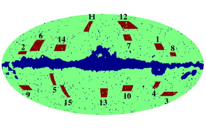
5 fields were chosen in which each of the three Galactic foregrounds were dominant. The synchrotron fields were selected from the Haslam et al. (1982) 408 MHz map, the free-free fields from the Dickinson et al. (2003) H$\alpha$ map and the dust fields from the SFD98 $100~{}\mu$m map. Table 2 lists the 15 fields of the present study. For each field the dominant emission and the Galactic coordinates are given along with a short description of the field.

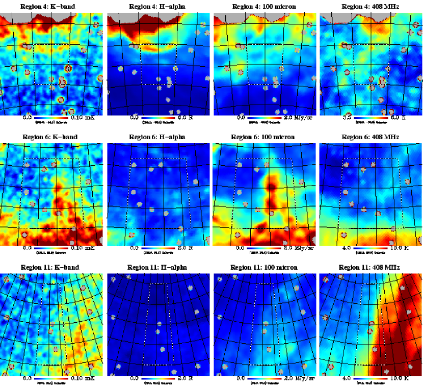
Fig. 2 shows the position of the 15 selected regions overlaid on the Kp2 intensity mask and source mask ($\sim 700$ sources in total) used by the WMAP team (Bennett et al. 2003b). Fig. 3 shows 3 regions (regions 4,6 and 11) with an ILC-subtracted K-band, H$\alpha$, $100~{}\mu$m and 408 MHz data. The dominant foreground in each region (see Table 2) is clearly seen along with the correlated emission at K-band.

Figure 3: Maps of region 4 (H$\alpha$ (free-free) dominated; top row), region 6 (dust dominated; middle row), and region 11 (synchrotron dominated; bottom row). From left to right are maps at WMAP K-band, H$\alpha$, SFD98 $100~{}\mu$m dust intensity and 408 MHz. Galactic coordinates are shown. Each map, with a pixel resolution $N_{side}=256$, covers a $25^{\circ}\times 25^{\circ}$ area with $1^{\circ}$ resolution. The dotted black/white line delineates the actual areas used for the T–T plots and cross-correlation analyses. Grey-areas are the standard WMAP Kp0 mask and extragalactic sources mask.

4 Cross-correlation analysis

The cross–correlation (C–C) method used here is a least–squares fit of one map to one or more templates. In the absence of any covariance information on the residuals, and assuming no net offsets (i.e. monopoles), this method is equivalent to the classical T–T method when only one template map ($T_{1}\equiv{\mathbf{t}}$) is compared to the data ($T_{2}\equiv{\mathbf{d}}$). The advantage of the C–C method is that we can fit several components simultaneously and that we can include information about the CMB thorough its signal covariance rather than having to correct for it. The issues of CMB subtraction and correlated components are discussed further in Appendices A & B.

4.1 Method

The cross–correlation measure, $\alpha$, between a data vector, ${\bf d}$ and a template vector ${\bf t}$ can be measured by minimising:

$$\chi^{2}=({\bf d}-\alpha{\bf t})^{T}\cdot{\bf M}^{-1}_{SN}\cdot({\bf d}-\alpha{\bf t})={\bf\tilde{d}}^{T}\cdot{\bf M}^{-1}_{SN}\cdot{\bf\tilde{d}}$$ (3)

where ${\bf M}_{SN}$ is the covariance matrix including both signal and noise for the template–corrected data vector ${\bf\tilde{d}}\equiv{\bf d}-\alpha{\bf t}$. Solving for $\alpha$ then becomes:

$$\alpha=\frac{{\bf t}^{T}\cdot{\bf M}^{-1}_{SN}\cdot{\bf d}}{{\bf t}^{T}\cdot{\bf M}^{-1}_{SN}\cdot{\bf t}}$$ (4)

To compare multiple template components ${\mathbf{t}}_{j}$, e.g., different foregrounds, to a given dataset, the problem becomes a matrix equation. Górski et al. (1996) describe the method in harmonic space, which is fundamentally no different from pixel space. In the case where we have $N$ different foreground components, we end up with the simple system of linear equations ${\bf Ax}={\bf b}$,where

$$A_{kj}=\mathbf{t}^{T}_{k}\cdot\mathbf{M}_{\textrm{SN}}^{-1}\cdot\mathbf{t}_{j},$$

$$b_{k}=\mathbf{t}^{T}_{k}\cdot\mathbf{M}_{\textrm{SN}}^{-1}\cdot\mathbf{d},$$

$$x_{k}=\alpha_{k}.$$ (5)

When only one template is present, this reduces to equation (4) above.

The signal covariance is that for theoretical CMB anisotropies, $M^{S}_{ij}=\frac{1}{4\pi}\sum^{\infty}_{\ell=0}(2\ell+1)C_{\ell}B^{2}_{\ell}P_{\ell}(\hat{n}_{i}\cdot\hat{n}_{j})$, where $B_{\ell}$ is the Gaussian beam of $1\degr$ FWHM. The power spectrum, $C_{\ell}$, is taken from the WMAP best fit $\Lambda$CDM power law spectrum (Bennett et al. 2003a). The noise covariance is determined from the uncorrelated pixel noise as specified for each pixel in the WMAP data, and subsequently convolved as described above.

For each of the fifteen regions, the data vector includes only those pixels of interest, and the covariance matrices are only the corresponding rows and columns. These regions vary in size from 230 to 1140 pixels at this resolution.

The errors $\delta\alpha_{k}$ are the square root of the diagonal of ${\bf A}^{-1}$. The simultaneous fitting of multiple template components allows us to deal with the fact that, though the regions are chosen to be dominant in one given component, they are not entirely free of the other components. The simultaneous fitting of multiple foreground components allows such cross–talk to be quantified.

4.2 Results of the cross-correlation analysis

At each WMAP band the emissivity of the 3 foreground components (free-free, dust and synchrotron) has been estimated as a ratio of template brightness; $\mu$K R^-1, $\mu$K/$\mu$K_FDS8 and $\mu$K K^-1 respectively. The analysis was a joint solution derived for all 3 components simultaneously. For each of the components we also made solutions for the all-sky (Kp2 cut) WMAP data.

4.3 Free-free emission

The 5 isolated regions with strong H$\alpha$ features ($1-5$) are listed in Table 2. Free-free emission should in principle be detectable at radio frequencies from 408 MHz up to and including the WMAP frequencies. Accordingly we have used the additional radio surveys at 1.4 GHz (Reich & Reich, 1988) and 2.3 GHz (Jonas et al. 1998) to confirm that the regions exhibit a general flattening of spectral index between 408 MHz and 2.3 GHz suggesting that there is considerable free-free emission, at least relative to any synchrotron component at these frequencies. The peak H$\alpha$ intensities in the 5 maps are in the range $10-40~{}R$. The results of the analysis for K- and Ka-bands, where free-free emission will be strongest, are given in Table 3. For comparison we list the fits for the two H$\alpha$ templates (DDD and F03) and find overall, there is good agreement between them. The results indicate a lower electron temperature of roughly $T_{e}=4000-5000$ K rather than the often-assumed $T_{e}=8000$ K. However, it is important to note that there is variation in this ratio by a factor of $\sim$2 from region to region. The average of the 5 fields is consistent with the high Galactic latitude solution (Kp2 cut).

Field	Template	$\frac{T_{\rm K}}{T_{\rm H_{\alpha}}}$	$\frac{T_{\rm Ka}}{T_{\rm H_{\alpha}}}$	Hα intensity
No.		$\mu$K R-1	$\mu$K R-1	range R
1	F03	11.3±4.8	9.8±4.4	1-10
	DDD	9.8±4.4	6.2±4.1
2	F03	4.7±3.0	0.7±2.8	3-15
	DDD	5.2±2.9	1.4±2.7
3	F03	5.5±3.0	3.1±2.6	2-14
	DDD	2.3±3.5	-1.7±3.2
4	F03	7.4±2.6	4.4±2.3	3-16
	DDD	7.2±2.1	1.2±1.1
5	F03	9.6±1.1	4.8±1.0	3-40
	DDD	10.1±1.2	5.1±1.1
Avg.	F03	8.6±0.9	4.4±0.8
	DDD	8.5±0.9	3.0±0.7
Kp2	F03	7.7±0.9	3.7±0.9
	DDD	7.5±0.9	3.6±0.9
	Te=4000K	8.0	3.6
	Te=5000K	8.9	4.1
	Te=6000K	9.8	4.5
	Te=7000K	10.6	4.9
	Te=8000K	11.4	5.2

Table 3: Free-free emission as determined by C–C method for K-and Ka-band WMAP data. Units are brightness temperature T ($\mu$K) relative to unit H$\alpha$ intensity $I_{H_{\alpha}}$ (R). The expected values are shown at the bottom from the predictions given by Dickinson et al. (2003) assuming different electron temperatures. The range of H$\alpha$ intensities in each region is also given in the last column. For each region, two templates are used: the Finkbeiner (2003) template, F03, or the Dickinson et al. (2003), DDD. Full sky fits, outside the Kp2 cut, are also shown; here, only a diagonal approximation to the covariance matrix is used, and the uncertainties are determined using simulations (see Appendix B) and the DDD template only.

4.4 Anomalous dust emission

The dust emissivity for all fields for the 5 WMAP frequency bands is given in Table 4. The emissivity is that relative to the FDS8 prediction for the W-band and is given separately for the raw WMAP data and for H$\alpha$ corrected data. Also shown is the range of dust temperature in each field taken from SFD98. The five fields ($6-10$) that were selected on the basis that they exhibited dust emission only weakly confused by synchrotron or H$\alpha$ (free-free) emission produced the most significant correlations amongst the 15 fields studied. In addition field numbers 2,5,11,14 and 15 also show significant dust correlations; this is because the anomalous dust emission is the dominant foreground at the lower WMAP frequencies ($20-40$ GHz). However, in these latter fields some confusion from synchrotron and free-free might have been expected. The possible effect of a contribution from free-free emission has been tested by subtracting the H$\alpha$ template converted to free-free brightness temperature with an electron temperature $T_{e}=4000$ K, consistent with our previous findings. The free-free correction is small relative to the dust and the dust results remain remarkably robust.

It can be seen from Table 4 that there is a spread of a factor of $\approx 2$ in the emissivity of dust clouds. The range of dust emission spectral index as determined for example by the ratio of K to Ka-band emissivity of individual clouds is less than this ($\sim 1.4$ in the dust-dominated regions) and may also be a significant result.

The spectrum of the the anomalous dust emissivity is best given by the average of the clouds listed in Table 4. The average values are seen to be slightly higher than that of the full-sky (Kp2 cut). Note that the traditional vibrational dust component is negligible in the K, Ka and Q-bands and is only dominant at W-band.

The anomalous dust emissivity, when corrected for vibrational emission, shows an average spectral index $\beta$ of $-2.85$ (varying from $\approx-2.8$ to $-3.8$ in the dust-dominated regions) and is discussed further in section 5.2.

Field	FDS range	Dust T range	Dust emissivity relative to FDS					Notes
No.	($\mu$K)	(K)	K	Ka	Q	V	W
1	4.4-10.3	17.6-18.5	8.4±5.9	-0.1±5.1	2.4±4.3	-1.0±3.3	-2.3±2.6
			8.9±5.7	0.5±5.0	3.4±4.2	-0.3±3.2	-1.6±2.5
2	14.2-41.3	16.5-17.5	6.6±1.6	1.8±1.3	2.0±1.2	-0.8±1.1	0.3±0.9
			6.2±1.6	0.9±1.3	0.5±1.2	-2.1±1.0	-0.3±0.9
3	1.6-10.1	17.6-18.5	12.1±5.2	5.5±4.5	7.2±3.9	4.8±3.5	-0.7±3.1
			7.7±4.7	1.6±4.1	3.8±3.6	2.7±3.3	-0.8±2.9
4	2.5-10.4	17.8-18.3	3.9±6.1	7.3±5.1	6.4±4.3	2.5±3.6	-2.0±3.0
			2.9±5.6	4.8±4.9	5.0±4.3	2.0±3.5	-2.3±3.0
5	6.9-30.2	17.2-18.6	12.6±2.1	2.6±1.8	2.6±1.6	-0.3±1.4	-0.8±1.2
			13.1±2.0	2.5±1.8	1.7±1.6	-1.6±1.4	-1.6±1.2
6	2.8-51.1	15.7-18.1	6.7±0.7	2.9±0.6	2.1±0.6	0.8±0.5	2.3±0.4
			6.5±0.7	2.6±0.6	1.9±0.6	0.8±0.5	2.2±0.4
7	6.2-17.0	17.9-18.7	8.1±3.9	2.8±3.5	0.2±3.2	0.6±2.9	0.5±2.6
			7.8±3.8	2.8±3.5	-0.3±3.2	0.4±2.9	0.2±2.6
8	6.4-25.8	17.1-18.0	8.4±2.5	2.6±2.3	2.4±2.2	2.4±2.0	3.1±1.8
			8.2±2.5	2.6±2.3	2.5±2.2	2.5±2.0	3.1±1.8
9	9.6-97.5	15.4-17.8	7.3±0.6	2.9±0.6	1.8±0.5	1.4±0.5	1.9±0.4
			7.3±0.6	2.9±0.6	1.8±0.5	1.4±0.5	1.9±0.4
10	3.5-31.7	16.8-18.3	12.0±1.4	4.7±1.2	1.8±1.1	0.2±1.0	1.3±0.9
			12.2±1.3	5.0±1.2	1.8±1.1	0.3±1.0	1.3±0.9
11	1.9-7.6	17.6-18.3	19.0±7.9	9.9±6.8	6.6±6.1	3.1±5.4	1.4±4.7
			17.8±7.8	8.3±6.7	7.0±6.1	3.5±5.4	1.3±4.7
12	2.2-5.9	17.6-18.2	15.6±7.5	5.3±6.6	4.6±5.8	-7.1±5.0	-2.1±4.2
			15.4±7.5	5.1±6.6	4.4±5.8	-7.3±5.0	-2.2±4.2
13	1.9-10.5	17.5-18.5	3.9±6.4	-3.7±5.7	1.6±4.9	-2.2±3.8	-1.0±3.1
			3.6±6.3	-3.0±5.7	1.5±4.9	-2.2±3.8	-1.0±3.1
14	3.7-9.8	17.5-18.5	8.3±4.8	7.6±3.9	1.8±3.0	3.0±2.3	-0.6±1.8
			7.1±4.7	7.1±3.9	1.1±3.0	2.2±2.3	-0.7±1.8
15	6.1-16.3	17.2-18.3	8.1±3.3	-1.0±3.0	-1.0±2.7	-1.3±2.5	-0.5±2.2
			8.1±3.3	-0.8±3.0	-0.9±2.7	-1.4±2.5	-0.4±2.2
Avg.			7.8±0.4	3.0±0.4	2.0±0.3	0.8±0.3	1.6±0.3
			7.7±0.4	2.8±0.4	1.8±0.3	0.6±0.3	1.4±0.3
Kp2			6.6±0.3	2.4±0.3	1.4±0.3	0.9±0.3	1.2±0.3
			6.6±0.3	2.4±0.3	1.4±0.3	0.8±0.3	1.1±0.3

Table 4: Dust-correlated emissivity in the 5 WMAP bands from a C–C analysis with the FDS model 8 dust prediction at 94 GHz. For each region, the first row gives the result from a simultaneous fit of the three foreground components, while the second row gives that for a fit of two foregrounds to data with the H$\alpha$ (free-free) subtracted assuming $T_{e}=4000$ K. Also shown are the FDS8 predicted dust emission intensity range for each region as well as the SFD dust temperature. The five dust-dominated regions are highlighted in bold face. Full sky fits, outside the Kp2 cut, are also shown; here, only a diagonal approximation to the covariance matrix is used, and the uncertainties are determined using simulations.

4.5 Synchrotron emission

The 408 MHz all-sky map is used as the basic synchrotron template for comparison with the WMAP data. The fits between the 408 MHz and the WMAP maps (bands K, Ka and Q) are given in the upper part of Table 5. The spectral index of synchrotron emission between the WMAP bands can be derived from the 408 MHz-correlated signal at each WMAP frequency and is given in the bottom part of Table 5. Note that the implied spectral index can be misleading where the synchrotron is not detected at an amplitude higher than its error bar (upper part of Table 5). It can be seen that, except of region 11 at K-band, the results for individual regions are not significant at the $2\sigma$ level. Nevertheless, these spectral index values are somewhat steeper than those calculated between GHz frequencies and the WMAP frequencies. This is likely to be due to the effect of spectral ageing of the CR electrons which produce the synchrotron emission in the Galactic magnetic field. The average of the five regions is significant at K-band with $\beta=-3.18$ and the full-sky value (outside of the Kp2 cut) is $-3.01$. The uncertainties shown for the Kp2 fits are based on simulations and are larger than might be expected since they use a diagonal approximation to the full covariance matrix M in equation (4) (see Appendix B for details).

	Synchrotron fit amplitudes ($\mu$K K-1)
Field	$\frac{K}{408}$	$\frac{Ka}{408}$	$\frac{Q}{408}$
11	$4.28^{\pm 1.76}$	$-0.02^{\pm 1.11}$	$-0.65^{\pm 0.77}$
12	$2.94^{\pm 1.64}$	$0.55^{\pm 0.63}$	$0.13^{\pm 0.26}$
13	$2.77^{\pm 2.02}$	$0.73^{\pm 0.83}$	$0.50^{\pm 0.40}$
14	$1.60^{\pm 1.54}$	$-0.36^{\pm 0.63}$	$-0.49^{\pm 0.31}$
15	$2.97^{\pm 2.78}$	$-0.82^{\pm 1.51}$	$-0.17^{\pm 0.91}$
Avg.	$2.82^{\pm 0.82}$	$0.15^{\pm 0.36}$	$-0.04^{\pm 0.17}$
Kp2	$5.56\pm 0.79$	$1.46\pm 0.78$	$0.50\pm 0.77$
	Synchrotron spectral index $\beta$
Field	$\frac{K}{408}$	$\frac{Ka}{408}$	$\frac{Q}{408}$
11	$-3.07^{+0.09}_{-0.13}$	$<-2.97$	$<-3.03$
12	$-3.17^{+0.11}_{-0.20}$	$-3.28^{+0.17}$	$-3.44^{+0.23}$
13	$-3.18^{+0.14}_{-0.32}$	$-3.22^{+0.17}$	$-3.15^{+0.13}_{-0.35}$
14	$-3.32^{+0.17}_{-0.81}$	$<-3.17$	$<-3.47$
15	$-3.16^{+0.16}_{-0.69}$	$<-2.97$	$<-2.89$
Avg.	$-3.18^{+0.06}_{-0.09}$	$-3.58^{+0.28}$	$<-3.27$
Kp2	$-3.01^{+0.03}_{-0.04}$	$-3.06^{+0.10}_{-0.18}$	$-3.15^{+0.20}$

Table 5: Synchrotron fits between 408MHz and the WMAP K, Ka, and Q bands. In the lower half of the table, the fit value is converted to a spectral index $\beta$ (T${}_{b}\propto\nu^{\beta}$), as are that value plus and minus the $1\sigma$ error bars (where positive). Where the fit amplitude is less than zero, the $2\sigma$ upper limit on the index is shown instead ($<2\sigma$).

5 Discussion

5.1 Free-free emission

Free-free emission is the weakest foreground component at WMAP frequencies for intermediate and high Galactic latitudes. By selecting five H$\alpha$-dominated regions, we have been able to quantify the H$\alpha$-correlated free-free emission in these regions as tabulated in section 4.3 (Table 3).

We note that the current analysis is for intermediate and high latitude Hii regions which are therefore associated with the local spiral arm such as the Gould Belt system and the Gum Nebula; they most likely lie at $|z|\stackrel{{\scriptstyle<}}{{{}_{\sim}}}200$ pc from the Galactic plane. This class of Hii regions is different from the more compact regions confined to the Galactic plane with a width of $z\approx 60$ pc (Paladini et al. 2003, 2004). As mentioned in section 2.2, these Hii regions have a mean $T_{e}=7200\pm 1200$ K compared to the value of around $4000-5000$ K found in the present study. Note that for the brightest region (5) where $T_{e}$ is most accurately determined, $T_{e}\sim 6500$ K. This discrepancy has an unclear origin, especially given that an identical result is determined for the entire high-latitude sky as defined by the WMAP Kp2 mask. It may be indicative of problems associated with the H$\alpha$ template itself, or in the conversion of H$\alpha$ flux to the free-free brightness temperature. However, variations by a factor of $\sim$2 are also seen from region to region.

It is of interest to note that the electron temperature derived from radio recombination line studies of extended Hii regions such as the Gum Nebula have an average value of $~{}7000$ K (Woermann, Gaylard & Otrupcek 2000). A study of diffuse foregrounds in the COBE-DMR at $7^{\circ}$ angular scales (Banday et al. 2003) found that H$\alpha$ correlations with the DDD H$\alpha$ template were more or less consistent with $T_{e}\sim 7000$ K for $|b|>15^{\circ}$. For $|b|>30^{\circ}$, lower values were preferred but with larger error bars. Banday et al. (2003) also analysed 19 GHz data with a $3^{\circ}$ beam, which favoured lower values even for $|b|>30^{\circ}$. These results suggest that the discrepancy may be scale-dependent and therefore might be related to the different beam shapes of the WHAM and SHASSA H$\alpha$ surveys for angular scales comparable to the beam size ($\sim 1^{\circ}$).

5.2 Dust emission

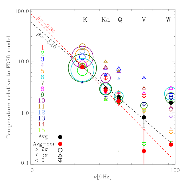
The dust-correlated emission is the dominant foreground component in the WMAP bands and its spectral properties can be derived for the individual clouds included in the present study. The spectra of all fifteen regions are shown in Fig. 4. It is immediately seen that the spectral slopes of each of the clouds over the range from K- to V-band are quite similar. Also, all the clouds show a turn-up in emissivity at W-band where thermal emission becomes dominant.

A further significant result is that the emissivity relative to the FDS8 prediction varies by a factor of 2 from cloud to cloud.

The average spectral emissivity for the clouds is shown by black filled circles in Fig. 4. The average spectral index from K- to Q-band, is $-2.4$, shown as a dashed black line in Fig. 4. The average spectral index in the range K–Ka-band and Ka–Q-band are $-2.6$ and $-1.9$. An estimate of $\beta$ from K-band to higher frequencies depends sensitively upon the vibrating dust contribution in these bands and requires a knowledge of its spectral index. Assuming $\beta=+1.7$, we use a simple $\chi^{2}$ test to find the best fit to the data over a grid of values for the anomalous dust spectral index, the anomalous dust amplitude, and the vibrating dust amplitude. The result gives a spectral index for the anomalous component of -2.85 and shows that the FDS8 prediction at W-band is underestimated by 30 per cent. Assuming a steeper thermal index of 2.0 or 2.2 results in an anomalous index of $-2.75$. The data minus the vibrating dust fit are shown in red in Fig. 4 along with the best-fit anomalous power law.

One proposed explanation for the anomalous dust-correlated emission in the low frequency WMAP bands, motivated by its spectral behaviour, is that it represents a hard synchrotron component, morphologically different in the WMAP bands from the soft synchrotron component traced by the 408 MHz emission. This hard synchrotron emission would correlate with dust in regions of active star formation. We find that this anomalous component has a spectral index from the K- to Q-band of $\beta=-2.85$ when the FDS8 thermal dust prediction is subtracted, assuming $\beta=+1.7$ (see Fig. 4). We then extrapolate this component to 408 MHz to see how much of this hard emission would be seen at that low frequency. If there is no spectral hardening between 408 MHz and WMAP, then a spectral index of $\beta=-2.85$ would imply more emission at 408 MHz than is observed by a factor of $\stackrel{{\scriptstyle>}}{{{}_{\sim}}}2$ in many regions. If the thermal dust spectrum is steeper, e.g., $\beta=+2.2$, then (as discussed above) the anomalous index flattens slightly to $-2.75$, but that still over-predicts the emission at 408 MHz.

Figure 4: Summary of dust emissivities (antenna temperature units, relative to FDS8 at 94 GHz) from C–C analysis. Each region emissivity is plotted with a different colour open symbol whose size is proportional to the signal-to-noise ratio. The symbol is a circle if the signal-to-noise is greater than two or a triangle if it is positive but less than two. Where the fit value is negative, the $1\sigma$ upper limit is shown as an arrow downward, and values more than one sigma negative are not shown (though all values are included in the weighted average). The filled black circle shows the weighted average surrounded by its error bar. The dashed line represents the best-fit spectral index over K through Q bands. Red filled circles and the red dashed line show the average and fit when corrected for the best-fit thermal dust component assuming $\beta=+1.7$; see text in §5.2.

We now consider the relevance of the dust temperature to our results, using as a proxy the SFD98 colour temperature based on the ratio of the DIRBE 100- and 240- $\mu$m data at a resolution of $1.\!^{\circ}1$.

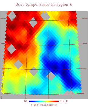
Comparing the dust temperature to the emissivity in these regions (as well as over the sky outside the Kp2 cut), it appears that in general, the strongest anomalous emission (relative to the FDS8 prediction) comes from the coldest regions. This is particularly striking in the two dust regions which have the smallest error bars, 6 and 9, which can be seen to dominate the averages in Table 4 and Fig. 4. Fig. 5 shows the dust temperature in region 6, which can be compared to the $100~{}\mu$m SFD98 map shown in Fig. 3. The fit amplitudes in these regions show the lowest cross-correlation with the low-frequency data, where the emission is not thermal but comes from the anomalous component. Table 4 shows that the K-band emission (where strongly detected) is lowest relative to the FDS8 template in regions 2, 6, and 9, which have the lowest dust temperatures as well. (Not apparent from the table, which shows only the dust temperature range, is that the emission comes from the coldest parts of the region).

Finkbeiner (2004) has examined the foreground residuals after subtracting the FDS8 prediction and proposed that an anomalous dust template could be better constructed using FDS8$\times{\rm T}^{2}$. By comparing the $\chi^{2}$ values for template fits for the Kp2 mask using FDS8$\times{\rm T}^{n}$ for different values of $n$, we find that formally the best value for $n$ in the K-band is $1.6$ and that it drops to zero at the higher frequencies, as one would expect. The same exercise repeated on the fifteen regions, however, gives a large scatter in the preferred value of $n$, ranging from 0 to over 5 (the limit of the range tested).

The average dust emissivity among all of the regions is slightly higher at low frequencies (particularly K-band) than that over the full sky (outside the Kp2 cut). Can this be explained by the full sky fits being driven by the even colder emission near the Galactic Plane at the anti-centre? Fits of the FDS8 template to the hemisphere around the Galactic centre and around the Galactic anti-centre do indeed show that the fit values around the anti-centre are from 10 to 30 per cent lower than fits around the Galactic centre, depending on the band. These differences appear to confirm the indication in the smaller regions that the emissivity of the anomalous component is lower from colder dust.

Figure 5: SFD dust temperature for region 6, showing that the emissivity, as seen in Fig. 3, comes from the coldest regions.

5.3 Synchrotron emission

As in the case of free-free emission the synchrotron emission, defined as the 408 MHz-correlated emission, is weaker than the dust-correlated emission at WMAP frequencies ($20-90$ GHz) over most of the sky. Except for the strongest synchrotron feature, the North Polar Spur (region 11), the 408-MHz correlations are marginal, even at K-band. Nevertheless the average spectral index of the 5 synchrotron-selected fields (Table 5) indicates an increasing slope relative to 408 MHz of $\beta=-3.18$ to $<-3.27$ from K to Q-band. The full-sky fits (Kp2) indicates $\beta=-3.01$ from 408 MHz to 23 GHz. At higher WMAP frequencies, the fits are not significant. The errors are probably too conservative due to the diagonal covariance assumption used in the Kp2 fit (see Appendix B). Nevertheless, the results are in good agreement with the WMAP values reported in Bennett et al. (2003b).

Using low frequency maps at GHz frequencies (408 MHz, 1420 MHz, 2326 MHz from Haslam et al. (1982), Reich & Reich (1986) and Jonas et al. (1998), respectively) we find that the average spectral index for the 5 maps in the GHz range is $-2.91$. This steepening with frequency is indicative of ageing of the relativistic electrons in these fields. This can be compared with the results of the Cosmosomas experiment which found $\beta~{}-3.16$ from 408 MHz to 13 GHz for $|b|>30^{\circ}$ (Fernández-Cerezo et al. 2006). Our limited data does not show evidence for strong variation of the synchrotron spectral index at WMAP frequencies from field-to-field. The discrepancy between the average of the regions and the Kp2 cut is likely to be due to the dominance of the North Polar Spur which is known to have a steeper index relative to the sky average.

6 Comparison with WMAP3

Whilst this paper was being completed, the WMAP team released their 3-year results to the community. For this new analysis, several semi-independent studies of the foreground contamination of the data were undertaken (Hinshaw et al. 2006). For the purposes of gaining physical insight into the nature of the Galactic foregrounds, a maximum-entropy (MEM) technique was applied. However, for the purposes of cleaning the data for cosmological studies, a template subtraction method was adopted. As with the first year analysis, the F03 H$\alpha$ template was employed as a tracer of free-free emission and the FDS8 model normalised at 94 GHz used for thermal dust emission. For synchrotron emission an internally generated template, comprising the difference of the K- and Ka-bands, was constructed. There are several aspects of these foreground results that merit comment in the present paper.

Hinshaw et al. (2006) have determined a free-free to H$\alpha$ ratio of $\sim$6.5 $\mu$K R^-1 based on fits to the F03 template. This is completely consistent with the mean values derived from the 5 free-free regions in this paper, particularly after adjusting the WMAP coefficient 20-30 per cent upwards to compensate for the increased amplitude of their $f_{d}=0.5$ dust corrected H$\alpha$ template. The MEM analysis finds a slightly higher ratio $\sim$8 $\mu$K R^-1, but also considerable variation (by a factor of $\sim$2) depending on location, as we have also found.

They adopted the difference between the observed K- and Ka-band emission as a tracer of synchrotron emission was intended to compensate for the problem with assuming a fixed full-sky spectral index in order to extrapolate the Haslam 408 MHz sky map to WMAP frequencies. Such a procedure is clearly in contradiction with the spectral index studies of Reich & Reich (1988) between 408 and 1420 MHz, which showed large variations of spectral index across the sky. Of course, utilising the K-Ka map as a foreground correction template is, to some extent, independent of whether the dominant foreground contribution is due to synchrotron, anomalous dust, or a combination thereof. By utilising what Hansen et al. (2006) have referred to as an internal template, it is likely that the synchrotron morphology is well traced over the frequencies of interest. Moreover, fitting this template to the remaining sky maps with a global scale factor per frequency is likely to be quite accurate, even in the presence of modest departures from a single spectral index. This treatment does not contradict our own studies, since our intention is to study the variations in spectral behaviour over the sky relative to the 408 MHz survey (Section 5.3).

Maintaining a consistent approach to their treatment of the first year data, the WMAP team have not attempted to directly address the issue of the anomalous dust correlated component. Rather, the MEM solutions were allowed only to produce what may be interpreted as a combined synchrotron/anomalous dust solution at each frequency, with no attempt made to disentangle the two components. Hinshaw et al. (2006) comment that it is not possible, using the WMAP data alone, to distinguish between anomalous dust emission and flatter spectrum synchrotron emission that is well correlated with dusty star-forming regions. This is particularly true given that a putative spinning dust component can exhibit a similar spectral shape to synchrotron emission over the 20 - 40 GHz frequency range. However, Page et al. (2006) in their foreground modelling efforts for the polarisation analysis, determine a high-polarisation fraction component of the synchrotron emission that is well correlated with the Haslam template, and a low-polarisation component with a dust-like morphology. We argue that this is indicative of a spinning dust component. Furthermore, an unexpected flattening of the spectral index for the polarised synchrotron emission was also found. It is important for understanding the foreground polarisation where the percentage polarisation is very different for each component.

Finally, we note that the WMAP team impose a constraint on their thermal dust template fits that the derived dust coefficients must have a spectral index of $\sim$2, rather than the value of 2.2 used in the first year analysis, or the value of 1.7 predicted by the FDS8 model. This makes only a very minor difference to the spinning dust spectrum because thermal dust emission is negligible at in the lowest WMAP bands.

7 Conclusions

In our study of the free-free, dust and synchrotron foreground components in the WMAP data we have chosen a selection of fields which are intended to have minimal cross-contamination from other components. Each of the 3 components has been quantified in terms of a mean value of the emissivity in each of the 5 WMAP bands.

Fig. 6 shows the emission, in thermodynamic units, as expected using the values of emissivity we have determined in conjunction with the H$\alpha$, 100 $\mu$m dust and the 408 MHz templates outside the Kp2 mask. These are calculated using r.m.s. values of 5.9 K, 2.6 R and $6.8~{}\mu$K for 408 MHz, H$\alpha$, and FDS8 model at 94 GHz, respectively. The data points are the Kp2 solutions from the C-C analysis. The curves are foreground models; synchrotron with $\beta=-3.1$ normalised to K-band, free-free with $\beta=-2.14$ for $T_{e}=4000$ K and vibrational dust emission for $\beta=+1.7$ normalised to W-band. The magenta curve is a spinning dust model from Draine & Lazarian (1998a,b), scaled to fit the data points from K- to Q-band. The curves plotted in Fig. 6 are therefore not strictly “best-fits” to these data points and are plotted to depict the approximate amplitude and spectral dependencies of the 4 Galactic components at high latitudes (outside the Kp2 cut). The dominance of the dust emission is evident. Also the similarity of the dust and the synchrotron spectrum at WMAP frequencies is superficially evident; these may be separated by lower frequency ($5-15$ GHz) data as shown for example by de Oliveira-Costa et al. (2004) and Watson et al. (2005). We note that dust (anomalous and thermal) is the dominant foreground over the WMAP and Planck bands. The thick black curve in Fig. 6 is the total of the 4 model curves, combined in quadrature, corresponding to the approximate total foreground r.m.s. level; the minimum foreground contamination of the CMB is at $\sim 70$ GHz for total intensity. The integrated foreground spectrum is relatively simple when sampled sparsely in frequency (e.g. WMAP). This is why the WMAP team find that the spectrum from 408 MHz to V-band is well-fitted by a simple power-law, although it says little in itself about the underlying foreground components.

Figure 6: R.m.s. fluctuations spectrum (thermodynamic temperature units) of foreground components at $1^{\circ}$ resolution. The symbols are the Kp2 solutions from the C–C analysis for synchrotron (blue squares), free-free (green triangles) and anomalous dust-correlated emission (magenta circles). The curves represent synchrotron for $\beta=-3.1$ (blue dotted line), free-free for $\beta=-2.14$ (green short dashed line), vibrational dust with $\beta=+1.7$ (red dot-dashed line), Draine & Lazarian spinning dust model (long dashed magenta line) and all the foreground models combined in quadrature (thick black line). The CMB fluctuations are shown at $70~{}\mu$K r.m.s (thin black line). The grey region shows the variation of dust emissivity between K- and Ka-bands in regions where significant ($>2\sigma$) dust-correlated emission was detected.

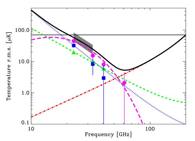
One of the most interesting results of the present study is the variation in the emissivity of the dust-correlated emission in the WMAP bands, typically by a factor of $\sim 2$. The grey shaded region of Fig. 6 indicates the variation of the dust-correlated component between K- and Ka-bands from the C-C analysis of 15 regions where a significant ($>2\sigma$) detection was found. There is clearly considerable variation in dust emissivity at K- and Ka-bands. Fig. 6 also shows that the average emissivity in the regions is higher than typical value seen outside the Kp2 cut (see Table 4). The effect on producing an anomalous dust template is profound because it is the dominant foreground between 20 and 60 GHz. If the anomalous dust emission is polarised at $\sim 10$ per cent this could approach the synchrotron emission as an important polarised foreground in the $20-60$ GHz range. These considerations are important for cleaning CMB maps from missions such as WMAP and Planck as well and high sensitivity ground-based experiments such as CLOVER and QUIET.

The WMAP team have instigated some debate over the origin of the anomalous dust correlated component, and have preferred an interpretation in terms of a hard synchrotron contribution from star-forming regions that are strongly associated with dust. The 5 synchrotron regions selected in this paper are dominated by well-known structures on the sky away from star-forming regions. As such, it might be expected that the derived synchrotron indices would be steep, and this is indeed the case. It is also expected that cross-talk with other physical components should be minimised. An important results is that anomalous emission was detected in 11 out of the 15 regions of studied here. We consider this to be strong evidence against a synchrotron origin for the anomalous component, although the exact nature of the dust emission mechanism requires lower frequency measurements to elucidate the detailed spectral behaviour. Certainly, the anomalous emission constitutes the dominant foreground component over the 20 – 60 GHz frequency range.

Further work is required to understand the origin of this variation in dust emissivity by using other physical properties of dust such as its size and temperature. New data in the critical radio frequency range $\sim 5-15$ GHz will be vital for a clearer definition of the anomalous dust spectrum. Polarisation data will be particularly important for understanding the physical mechanism that produces the anomalous emission which is expected to be polarised at different levels (e.g. Draine & Lazarian 1999). For example, spinning dust emission is expected to be only weakly polarised, whereas the synchrotron emission is known to be highly polarised.

Appendix A Aliasing of foregrounds due to CMB subtraction

Some studies of the WMAP data remove the ILC map before performing the correlation analysis in order to minimise the impact of the CMB structure on that analysis. However, this introduces a new problem. The ILC is constructed as a linear combination of the five WMAP frequency bands in such a way that i) the CMB signal is conserved; ii) the variance of the final map is minimised. The latter condition does not guarantee the absence of residual foregrounds from the ILC. Therefore, when one subtracts the ILC from the individual WMAP frequency maps the foreground contribution is altered by an amount depending on the residuals in the ILC map. Since we do not know a priori the actual properties of the foregrounds present in the data, it is not possible to absolutely correct for the effect of this ’aliasing’ of foregrounds from the ILC into the individual frequency maps. However, as shown in Eriksen et al. (2004), the likely residual level can be predicted under various assumptions about the foreground spectral behaviour. This at least gives some insight into the impact of the ILC subtraction on derived foreground properties.

For the high latitude fields considered in this paper, the 5 coefficients that define the ILC map for each frequency band are constant. This allows us to calculate the effect of the ILC subtraction, for a given spectral index, both in terms of relative amplitude of the aliased signal as well as the effect on the derived spectral index.

The numbers in Table 6 represent the fraction of foreground signal present in the corrected frequency map in antenna temperature units, assuming a specific spectral behaviour for that foreground. The CMB correction due to the ILC is given by 0.109K$-$0.684Ka$-$0.096Q$+$1.921V$-$0.250W. For these coefficients, it turns out that the effect can be relatively small for some of the foregrounds and frequencies of the WMAP data. For example, a synchrotron component, with $\beta=-3.1$ is increased at the 3 per cent level at K-band or 10 per cent at Ka-band. For synchrotron, the strong aliasing at high frequencies is not important since the actual foreground level is well below that of the other components. For H$\alpha$, with a flatter spectral index, the effect is $\sim$1 per cent lower at K-band and $\sim$15 per cent at W-band. It appears that the K-, Ka- and Q-band fits are reliable tracers of the synchrotron and free-free spectral indices up to a modest correction factor. The anomalous emission appears to have a relatively steep spectral index similar to that of synchrotron thus we might expect aliasing at similar levels to the synchrotron emission for $\beta=-2.85$. This may not be the case if the spinning dust models of Draine & Lazarian are correct models of the emission mechanism.

The aliasing effect is most strongly seen in W-band for the vibrational dust component. For $\beta=+2.0$, the dust component will be reduced by as much as 40 per cent. This is enough to change the effective spectral index of this component by a significant amount; a true spectral index of $+1.7$ increases to $+1.9$ after ILC subtraction. Furthermore, the dust correlation coefficients at low frequency have oversubtracted thermal dust contributions.

It is our contention that making an ILC subtraction before foreground analysis introduces difficulties of interpretation that may invalidate conclusions unless the effect of foreground aliasing is handled correctly.

$\beta$	K	Ka	Q	V	W
Free-free
-2.0	0.98	0.96	0.93	0.86	0.71
-2.1	0.99	0.98	0.97	0.93	0.84
-2.2	1.00	1.00	1.00	0.99	0.99
Thermal dust
1.7	-5.19	-2.25	-1.24	-0.08	0.54
2.0	-6.97	-2.75	-1.43	-0.03	0.62
2.2	-8.34	-3.08	-1.54	0.00	0.66
Anomalous dust
-2.5	1.02	1.05	1.08	1.21	1.53
CNM	1.09	1.08	1.09	1.24	3.59
WNM	1.28	1.41	1.69	5.41	436.00∗
WIM	1.28	1.32	1.46	3.01	62.10
Synchrotron
-2.7	1.03	1.07	1.12	1.35	1.98
-2.9	1.03	1.09	1.16	1.49	2.51
-3.1	1.03	1.10	1.19	1.62	3.09

Table 6: The fraction of foreground signal present in the corrected frequency map in antenna temperature units, assuming a specific spectral behaviour for that foreground. For example,. the Q-band contains 119 per cent of the synchrotron contribution expected if the synchrotron emission has a spectral index of $\beta=-3.1$. Therefore, in the absence of cross-talk with other foreground components, a synchrotron template fit to the Q-band should be downweighted by a factor of 1.19. For anomalous dust, we also tabulate the expected aliasing signal for the Cold Neutral Medium (CNM), Warm Neutral Medium (WNM), and Warm Ionised Medium (WIM) from models due to Draine & Lazarian (1998a,b). ^∗The W-band aliasing factor is large, but since the WNM spectrum falls off very rapidly this factor results only in physical amplitudes closer to the other channels.

Appendix B The reliability of T–T versus C–C fits

The T–T method is a straightforward linear fit of two datasets and has two basic drawbacks: firstly, only one template can be compared to the data, and secondly, only independent pixel noise (effectively, a diagonal covariance matrix) can be taken into account. The fifteen regions were chosen such that one component is dominant in an effort to get around the first problem. The ILC can be subtracted from the data in order to deal with the second. The C–C method is more complicated but allows simultaneous fitting of multiple templates with a full signal covariance matrix.

We use simulations with foreground components added at known amplitudes to test how well these different fitting methods recover the input. A set of 1000 simulations are created at the resolution of the WMAP data products, i.e. at HEALPix of $N_{\textrm{s}ide}=512$, using the beam width and noise properties of the respective channels. The foregrounds are added at the theoretical levels for free-free (assuming an electron temperature of T_e=8000 K) and for synchrotron (assuming a spectral index of $\beta=-3.0$), while the dust is added at the levels found by Table 3 of Bennett et al. (2003b), approximating both thermal and anomalous contributions. These maps are then smoothed (via convolution in harmonic space) to a common resolution of $1\degr$ and downgraded to $N_{\textrm{s}ide}=128$, as are the data.

These simulations can be used to test how much cross-talk still affects fits using only one template in the small regions chosen in an attempt to minimize such problems. In other words, does the existence of small amounts of additional dust and synchrotron emission in the H_α-dominated regions affect the individual fits using the H_α template alone? Looking at the elements of the fit matrix $A$ (defined in §4.1) gives an indication of how the different templates correlate with each other. This is shown for a few regions in Table 7. But analysis of simulations is needed to quantify the effects on the fit results.

First, we compare fits to data where the ILC estimate of the CMB component is subtracted, which is necessary in the T–T method but which introduces the small aliasing effects discussed in Appendix A. Table 8 columns labeled “1to3” give results where one template is fit to simulations with three foregrounds; these show that the H_α estimates are overestimated due to the other emission, even in regions dominated by H_α emission. The amount depends on the region, but some regions are overestimated by as much as 30%. This affects both methods when only one template is used. But where the C–C method is given the three templates to fit simultaneously, the results are then roughly consistent with the input, as seen in columns labeled “3to3”. The C–C and T–T methods also both give roughly correct results when only one foreground component is present in the data, as seen in the “1to1” columns.

The bias due to the ILC subtraction is clear in Table 8 in the “1to1” columns or the first “3to3” column. As expected for an index of $\beta=-2.1$, the free-free emission is underestimated by $\sim 1\%$. Likewise, the synchrotron is overestimated by approximately 3%. The dust is underestimated by $\sim 6\%$, as expected for the mixture of thermal and anomalous dust represented by the input amplitudes, taken from the WMAP best fits (Bennett et al. 2003b, Table 3.)

We conclude from the above and from the information in Table 8 that the only unbiased estimate of the foreground fit amplitudes comes from the full C–C method using the three template simultaneously and the CMB signal plus noise covariance matrix against the raw data. The bias introduced by the ILC-subtraction is relatively small (if the foregrounds follow roughly the expected spectral behavior), but the cross-talk among templates prevents the T–T method from being accurate enough in most cases. Only the C–C method with the full covariance, shown in the “3to3^†” column of Table 8 gives unbiased results.

In addition to template fitting in small regions, we have also tested the C–C method on the full sky outside the Kp2 mask. Only at very low resolution ($N_{\rm side}<=32$) can we use the full pixel-to-pixel covariance matrix, since higher resolution requires storing and inverting a matrix of $\sim$2GB, which is computationally prohibitive. For our analysis at $N_{\rm side}=128$, we simply use the diagonal of the full matrix. Using the same set of simulations described above, we can test how well this method works at recovering the input template amplitudes. Unlike the case where the full matrix is used, the diagonal of the matrix $\bf{A}$ does not give an accurate estimate of the uncertainty in the result, so these simulations are also necessary to quantify the distributions. We find that the method is unbiased, returning the correct mean for each template amplitude. The uncertainties are larger than they would be if we could use the full covariance matrix; using the diagonal makes the method much less accurate. This accounts for the fact that the errors shown in Tables 3 through 5 for the averages over all the regions are comparable to those given for the Kp2 fits despite the fact that if the same method could be used in both cases, the Kp2 fits would have smaller uncertainties.

	FDS dust	DDD Hα	Haslam	Const.
Region 5
FDS dust	1.00	0.23	0.59	0.62
DDD Hα	0.23	1.00	0.20	0.14
Haslam	0.59	0.20	1.00	0.82
Const.	0.62	0.14	0.82	1.00
Region 9
FDS dust	1.00	0.26	0.33	0.30
DDD Hα	0.26	1.00	0.42	0.44
Haslam	0.33	0.42	1.00	0.91
Const.	0.30	0.44	0.91	1.00
Region 14
FDS dust	1.00	0.34	0.51	0.61
DDD Hα	0.34	1.00	0.29	0.33
Haslam	0.51	0.29	1.00	0.73
Const.	0.61	0.33	0.73	1.00

Table 7: Fit matrix showing effectively the amount of cross-correlation among the different templates. Each value is $t^{T}_{i}M^{-1}t_{j}/\sqrt{(t^{T}_{i}M^{-1}t_{i})(t^{T}_{j}M^{-1}t_{j})}$. The regions were chosen as those where the dominant component had the smallest error bar.

Average fit amplitude as fraction of true
	TT…		CC…
	1to3	1to1	1to3	1to1	3to3	1to3†	3to3†
free-free (at $11.4~{}\mu$K R-1)
1	1.02$\pm 0.11$	0.99$\pm 0.11$	1.03$\pm 0.10(0.10)$	0.99$\pm 0.10(0.10)$	0.99$\pm 0.10(0.11)$	1.12$\pm 0.33(0.34)$	1.00$\pm 0.34(0.35)$
2	1.08$\pm 0.09$	0.99$\pm 0.09$	1.18$\pm 0.07(0.08)$	0.99$\pm 0.07(0.08)$	0.99$\pm 0.08(0.09)$	1.13$\pm 0.13(0.16)$	1.00$\pm 0.14(0.16)$
3	1.21$\pm 0.07$	0.99$\pm 0.07$	1.21$\pm 0.07(0.07)$	0.99$\pm 0.07(0.07)$	0.99$\pm 0.09(0.09)$	1.09$\pm 0.16(0.17)$	0.99$\pm 0.17(0.18)$
4	1.14$\pm 0.06$	0.99$\pm 0.06$	1.14$\pm 0.05(0.06)$	0.99$\pm 0.05(0.06)$	0.99$\pm 0.07(0.08)$	1.08$\pm 0.16(0.17)$	1.01$\pm 0.17(0.18)$
5	1.32$\pm 0.03$	0.99$\pm 0.03$	1.25$\pm 0.03(0.03)$	0.99$\pm 0.03(0.03)$	0.99$\pm 0.03(0.03)$	1.04$\pm 0.06(0.06)$	1.00$\pm 0.06(0.06)$
dust (at $6.3~{}\mu$K $\mu$K${}^{-1}_{FDS8}$)
6	1.06$\pm 0.03$	-	1.07$\pm 0.03(0.03)$	-	0.94$\pm 0.03(0.03)$	1.05$\pm 0.11(0.11)$	1.00$\pm 0.11(0.11)$
7	1.05$\pm 0.22$	-	1.06$\pm 0.22(0.22)$	-	0.94$\pm 0.23(0.25)$	1.13$\pm 0.59(0.60)$	1.00$\pm 0.59(0.61)$
8	0.87$\pm 0.15$	-	0.89$\pm 0.15(0.16)$	-	0.93$\pm 0.15(0.16)$	0.98$\pm 0.36(0.37)$	1.01$\pm 0.36(0.37)$
9	0.98$\pm 0.05$	-	0.98$\pm 0.05(0.05)$	-	0.94$\pm 0.05(0.06)$	1.03$\pm 0.10(0.10)$	0.99$\pm 0.10(0.10)$
10	1.03$\pm 0.06$	-	1.03$\pm 0.06(0.06)$	-	0.94$\pm 0.06(0.06)$	1.10$\pm 0.20(0.21)$	1.00$\pm 0.21(0.22)$
synchrotron (at $5.73~{}\mu$K K${}^{-1}_{408MHz}$)
11	1.32$\pm 0.08$	-	1.31$\pm 0.08(0.08)$	-	1.04$\pm 0.11(0.13)$	1.11$\pm 0.27(0.28)$	1.01$\pm 0.28(0.29)$
12	1.15$\pm 0.09$	-	1.15$\pm 0.09(0.09)$	-	1.03$\pm 0.10(0.10)$	1.05$\pm 0.24(0.26)$	1.01$\pm 0.24(0.26)$
13	1.24$\pm 0.13$	-	1.24$\pm 0.12(0.13)$	-	1.03$\pm 0.15(0.16)$	1.08$\pm 0.32(0.35)$	1.02$\pm 0.32(0.35)$
14	1.22$\pm 0.07$	-	1.22$\pm 0.06(0.06)$	-	1.04$\pm 0.08(0.09)$	1.08$\pm 0.23(0.24)$	1.00$\pm 0.23(0.24)$
15	0.65$\pm 0.18$	-	0.66$\pm 0.17(0.19)$	-	1.01$\pm 0.23(0.25)$	0.90$\pm 0.44(0.45)$	1.01$\pm 0.44(0.45)$

Table 8: Comparison of resulting fit amplitudes as fraction of true (see text). The expected foreground residuals after ILC subtraction in the K-band are: for free-free, assuming $\beta=-2.1$, 0.99% ; for dust, added at the WMAP best-fit values, approximating a combination of thermal and anomalous dust, 0.94%; for synchrotron, assuming $\beta=-3.0$, 1.03%. ^†C–C fits using the full covariance matrix.

Appendix C Full fit results

Field	K	Ka	Q	V	W
	free-free
1	9.8±4.4	6.2±4.1	6.0±3.9	3.4±3.6	3.7±3.2
2	5.2±2.9	1.4±2.7	0.3±2.6	-0.3±2.5	0.7±2.2
3	2.3±3.5	-1.7±3.2	-2.2±3.0	-2.5±2.8	0.8±2.5
4	7.2±2.1	1.2±1.1	0.9±0.6	0.3±0.4	-0.2±0.3
5	10.1±1.2	5.1±1.1	3.3±1.0	1.6±0.9	0.7±0.8
6	-4.7±9.9	-12.3±7.4	-12.1±6.3	-5.1±5.8	-10.9±5.2
7	3.5±11.9	6.8±9.0	-5.7±7.8	-0.5±7.2	-5.2±6.5
8	-22.9±16.4	0.7±13.5	-5.4±12.3	2.5±11.3	-13.1±10.2
9	9.2±15.5	-0.3±11.0	11.4±9.5	-1.2±8.7	0.1±7.9
10	15.3±15.2	13.6±7.2	2.7±3.9	5.7±2.3	1.1±1.7
11	-16.6±19.1	-29.4±13.2	12.9±11.5	9.6±10.4	-2.9±9.3
12	9.0±12.9	1.6±9.8	-9.6±8.4	-7.3±7.7	-5.2±7.0
13	3.7±14.0	15.1±7.2	-3.5±3.7	-1.5±2.2	-0.6±1.7
14	-4.4±8.0	-2.2±5.8	-1.2±4.9	-4.9±4.5	5.8±4.0
15	4.7±17.5	19.5±12.5	9.5±10.6	-9.5±9.7	2.6±8.7
	dust
1	8.4±5.9	-0.1±5.1	2.4±4.3	-1.0±3.3	-2.3±2.6
2	6.6±1.6	1.8±1.3	2.0±1.2	-0.8±1.1	0.3±0.9
3	12.1±5.2	5.5±4.5	7.2±3.9	4.8±3.5	-0.7±3.1
4	3.9±6.1	7.3±5.1	6.4±4.3	2.5±3.6	-2.0±3.0
5	12.6±2.1	2.6±1.8	2.6±1.6	-0.3±1.4	-0.8±1.2
6	6.7±0.7	2.9±0.6	2.1±0.6	0.8±0.5	2.3±0.4
7	8.1±3.9	2.8±3.5	0.2±3.2	0.6±2.9	0.5±2.6
8	8.4±2.5	2.6±2.3	2.4±2.2	2.4±2.0	3.1±1.8
9	7.3±0.6	2.9±0.6	1.8±0.5	1.4±0.5	1.9±0.4
10	12.0±1.4	4.7±1.2	1.8±1.1	0.2±1.0	1.3±0.9
11	19.0±7.9	9.9±6.8	6.6±6.1	3.1±5.4	1.4±4.7
12	15.6±7.5	5.3±6.6	4.6±5.8	-7.1±5.0	-2.1±4.2
13	3.9±6.4	-3.7±5.7	1.6±4.9	-2.2±3.8	-1.0±3.1
14	8.3±4.8	7.6±3.9	1.8±3.0	3.0±2.3	-0.6±1.8
15	8.1±3.3	-1.0±3.0	-1.0±2.7	-1.3±2.5	-0.5±2.2
	synchrotron
1	3.3±2.4	0.7±1.0	-0.7±0.5	0.0±0.3	-0.1±0.2
2	8.2±3.5	0.4±1.5	-0.9±0.8	0.8±0.5	0.7±0.4
3	3.7±2.2	1.3±0.8	0.4±0.4	-0.0±0.2	-0.1±0.2
4	4.2±3.0	1.2±1.0	1.0±0.5	0.5±0.3	0.1±0.2
5	4.3±2.2	1.7±1.1	-0.2±0.7	-0.7±0.4	0.1±0.3
6	2.8±1.3	-0.3±0.4	0.1±0.2	-0.2±0.1	-0.2±0.1
7	3.8±2.6	0.6±1.0	-0.5±0.5	-0.1±0.4	0.3±0.3
8	7.2±4.2	0.6±2.2	0.0±1.5	-0.2±1.0	0.4±0.8
9	0.2±3.3	0.1±1.6	2.1±1.0	-0.5±0.6	-0.5±0.5
10	1.2±2.1	0.8±0.9	-0.4±0.5	0.6±0.3	0.1±0.2
11	4.3±1.8	-0.0±1.1	-0.6±0.8	0.1±0.6	0.6±0.5
12	2.9±1.6	0.6±0.6	0.1±0.3	0.1±0.1	0.1±0.1
13	2.8±2.0	0.7±0.8	0.5±0.4	0.0±0.2	0.0±0.2
14	1.6±1.5	-0.4±0.6	-0.5±0.3	-0.0±0.2	-0.0±0.1
15	3.0±2.8	-0.8±1.5	-0.2±0.9	-0.4±0.6	-0.7±0.5

Table 9: Full fit results for all components in all regions. The three templates (DDD H_α, FDS8 dust, and Haslam 408MHz, plus a constant offset) are fit simultaneously to each band individually.

References

- (1) Banday A.J., Dickinson C., Davies R.D., Davis R.J., Górski K.M., 2003, MNRAS, 345, 897
- (2) Bennett C.L. et al., 2003a, ApJS, 148, 1
- (3) Bennett C.L. et al., 2003b, ApJS, 148, 97
- (4) Casassus S., Readhead A.C.S., Pearson T.J., Nyman L.A., Shepherd M.C., Bronfman L., 2003, ApJ, 591, 556
- (5) Condon J.J., Cotton W.D., Greisen E.W., Yin Q.F., Perley R.A., Taylor G.B., Broderick J.J., 1998, AJ, 115, 1693
- (6) de Oliveira-Costa A. et al., 1999, ApJ, 527, L9
- (7) de Oliveira-Costa A. et al., 2000, ApJ, 542, L5
- (8) de Oliveira-Costa A. et al., 2002, ApJ, 567, 363
- (9) de Oliveira-Costa A., Tegmark M., Davies R.D., Gutiérrez C.M., Lasenby A.N., Rebolo R., Watson R.A., 2004, ApJ, 606, L89
- (10) Davies R.D., Watson R.A., Gutierrez C.M., 1996, MNRAS, 278, 925
- (11) Dennison B., Simonetti J.H., Topasna G.A., 1998, PASP, 15, 147
- (12) Dickinson C., Davies R.D., Davis R.J., 2003, MNRAS, 341, 369 (DDD)
- (13) Draine B.T., Lazarian A., 1998a, ApJ, 494, L19
- (14) Draine B.T., Lazarian A., 1998b, ApJ, 508, 157
- (15) Draine B.T., Lazarian A., 1999, ApJ, 512, 740
- (16) Eriksen H.K., Banday A.J., Górski K.M., Lilje, P.B., 2004, ApJ, 612, 633
- (17) Fernández-Cerezo S. et al., 2006, MNRAS, submitted (astro-ph/0601203)
- (18) Finkbeiner D.P., 2003, ApJS, 146, 407 (F03)
- (19) Finkbeiner D.P., 2004, ApJ, 614, 186
- (20) Finkbeiner D.P., Davis M., Schlegel D.J., 1999, ApJ, 524, 867 (FDS)
- (21) Finkbeiner D.P., Schlegel D.J., Curtis F., Heiles C., 2002, ApJ, 566, 898
- (22) Finkbeiner D.P., Langston G.I., Minter A.H., 2004, ApJ, 617, 350
- (23) Gaustad J.E., McCullough P.R., Rosing W., Van Buren D., 2001, PASP, 113, 1326
- (24) Giardino G., Banday A.J., Fosalba P., Górski K.M., Jonas J.L., O’Mullane W., Tauber J., 2001, A&A, 371, 708
- (25) Górski, K. M. et al. 1996, ApJL, 464, L11 Górski K.M., Hivon E., Banday A.J., Wandelt B.D., Hansen F.K., Reinecke M., Bartelmann M., 2005, ApJ, 622, 759
- (26) Haffner L.M., Reynolds R.J., Tufte S.L., Madsen G.J., Jaehnig K.P., Percival J.W., 2003, ApJS, 149, 405
- (27) Hansen F.K., Banday A.J., Górski K.M., 2004, MNRAS, 354, 641
- (28) Hansen F.K., Banday A.J., Eriksen H.K., Górski K.M., Lilje, P.B., 2006, ApJ, submitted, astro-ph(0603308)
- (29) Haslam C.G.T., Klein U., Salter C.J., Stoffel H., Wilson W.E., Cleary M.N., Cooke D.J., Thomasson P., 1981, A&A, 100, 209
- (30) Haslam C.G.T., Stoffel H., Salter C.J., Wilson W.E., 1982, A&AS, 47, 1
- (31) Hinshaw, G. et al., 2003, ApJS, 148, 135
- (32) Hinshaw, G. et al., 2006, ApJ, submitted (astro-ph/0603451)
- (33) Jarosik N. et al., 2003, ApJS, 148, 29
- (34) Jonas J.L., Baart E.E., Nicolson G.D., 1998, MNRAS, 297, 977
- (35) Jones A.W., Davis R.J., Wilkinson A., Giardino G., Melhuish S.J., Asareh H., Davies R.D., Lasenby A.N., 2001, MNRAS, 327, 545
- (36) Kogut A. et al., 1996, ApJ, 464, L5
- (37) Lagache G., 2003, A&A, 405, 813
- (38) Lawson K.D., Mayer C.J., Osborne J.L., Parkinson M.L., 1987, MNRAS, 225, 307
- (39) Leitch E.M., Readhead A.C.S., Pearson T.J., Myers S.T., 1997, ApJ, 486, L23 Page L. et al., 2003, ApJS, 148, 39 Page L. et al., 2006, ApJ, submitted (astro-ph/0603450)
- (40) Paladini R., Burigana C., Davies R.D., Maino D., Bersanelli M., Cappellini B., Platania, P., Smoot G., 2003, A&A, 397, 213
- (41) Paladini R., Davies R.D., De Zotti G., 2004, MNRAS, 347, 237
- (42) Pauliny-Toth I.K., Shakeshaft J.R., 1962, MNRAS, 124, 61
- (43) Reich P., Reich W., 1986, A&AS, 63, 205
- (44) Reich P., Reich W., 1988, A&A, 196, 211 Shaver P.A., McGee R.X., Newton L.M., Danks A.C., Pottasch S.R., 1983, MNRAS, 204, 53
- (45) Schlegel D.J., Finkbeiner D.P., Davis M., 1998, ApJ, 500, 525 (SFD98)
- (46) Smoot G.F. et al., 1992, ApJ, 396, L1
- (47) Watson R.A., Rebolo R., Rubiño-Martin J.A., Hildebrandt S., Gutièrrez C.M., Fernàndez-Cerezo S., Hoyland R.J., Battistelli E.S., 2005, ApJ, 624, L89
- (48) Woermann B., Gaylard M.J., Otrupcek R., MNRAS, 2000, 315, 241
- (49) Wood K., Mathis J.S., 2004, MNRAS, 353, 1126