Oscillation mode lifetimes in $\xi\,$Hydrae: Will strong mode damping limit asteroseismology of red giant stars?

We introduce a new method to measure frequency separations and mode lifetimes of stochastically excited and damped oscillations, so-called solar-like oscillations. Our method shows that velocity data of the red giant star $\xi\,$Hya (Frandsen et al. 2002) support a large frequency separation between modes of roughly $7\,\mu$Hz. We also conclude that the data are consistent with a mode lifetime of 2 days, which is so short relative to its pulsation period that none of the observed frequencies are unambiguous. Hence, we argue that the maximum asteroseismic output that can be obtained from these data is an average large frequency separation, the oscillation amplitude and the average mode lifetime. However, the significant discrepancy between the theoretical calculations of the mode lifetime (Houdek & Gough 2002) and our result based on the observations of $\xi\,$Hya, implies that red giant stars can help us better understand the damping and driving mechanisms of solar-like p-modes by convection.

1 Introduction

The mode lifetime of solar-like oscillations is an important parameter. The interpretation of the measured oscillation frequencies (and their scatter) relies very much on knowing the mode lifetime, but currently we know very little about how this property depends on the stellar parameters (mass, age and chemical composition). The theoretical estimates of mode lifetimes are based on a simplified description of the convective environment in which the damping and excitation of the modes takes place. Measurements of the mode lifetime, $\tau$, in different stars will be very helpful for a more thorough treatment of convection in stellar modeling. In this paper the mode lifetime refers to the time for the amplitude to decrease by a factor of $e$.

The number of measurements of the mode lifetime, or damping time, is still very limited. Observations of main-sequence stars imply mode lifetimes of a few days in the Sun (Libbrecht 1988; Chaplin et al. 1997), $\alpha\,$Cen A (Bedding et al. 2004) and $\alpha\,$Cen B (Kjeldsen et al. 2005). As pointed out by Bedding et al. (2005b), independent observational studies on the star Procyon do not agree on the measured frequencies, a disagreement that could be the result of a short mode lifetime. The power spectrum of the K giant Arcturus reported by Retter et al. (2003) could also be explained as a short mode lifetime ($\tau=2\,$days) of a single mode. If the mode lifetime does not increase with oscillation period, this would limit the prospects of asteroseismology on evolved stars that have periods of several hours or longer, because of poor coherence of the oscillations. Only when we look at M giants – the semi-regular variables – do we see evidence for longer lifetimes, ranging from years to decades (Christensen-Dalsgaard et al. 2001; Bedding et al. 2003, 2005a).

The theoretical predictions of mode lifetimes for unevolved stars like the Sun (Houdek et al. 1999) and $\alpha$ Cen A (Samadi et al. 2004) are in a fairly good agreement with the observed values. However, for the more evolved red giant star $\xi\,$Hya, there seems to be a significant discrepancy between theory ($\tau\sim 15$–20 days; Houdek & Gough 2002) and observation ($\tau\sim 2$–3 days; Stello et al. 2004, hereafter Paper I). In Paper I we also measured the oscillation amplitude to be roughly $2\,$ms^-1, which was in good agreement with the theoretical value (Houdek & Gough 2002).

Figure 1: The oscillation ‘quality’ factor vs. period for selected stars. Filled symbols are measured, while the empty symbol shows the theoretical value. The arrow indicates a lower limit. Luminosity classes are indicated at the top. The measured values are from: $\alpha\,$Cen B, Kjeldsen et al. (2005); Sun, Chaplin et al. (1997); $\alpha\,$Cen A, Kjeldsen et al. (2005); $\xi\,$Hya (theoretical), Houdek & Gough (2002); $\xi\,$Hya (observed), Paper I; Arcturus, Retter et al. (2003); L₂ Pup, Bedding et al. (2005a); SV Lyn and R Dor, Dind (2004).

In Fig. 1 we plot the measured ratios between the mode lifetime and period (the oscillation ‘quality’ factor) as a function of period for selected stars, including the theoretical value for $\xi\,$Hya. Roughly speaking, the ‘quality’ factor is the number of oscillation cycles with constant phase, and the higher this number, the better we can determine the frequency. Note that the relation between the mode lifetime $\tau$ and the the FWHM $\Gamma$ (in cyclic frequency) of the corresponding resonant peak is $\Gamma=1/(\pi\tau)$.

In this paper we further investigate the mode lifetime of $\xi\,$Hya and examine whether it limits the possible astrophysical output. We introduce a new method that measures repeated frequency patterns (e.g. the large frequency separation, $\Delta\nu_{0}$) and the mode lifetime of solar-like p-mode oscillations. We furthermore analyze the stellar power spectrum to establish the most likely mode lifetime, by comparing the cumulative power distribution of the observations with simulations. Finally, the ambiguity of the measured frequencies is quantified.

2 The $\xi\,$Hya data set and previous results

We use the same data set as in Paper I, which comprises 433 measurements of radial velocity covering almost 30 days of single-site observations using the Coralie spectrograph at La Silla (ESO, Chile). The average noise per measurement is $\sigma_{\mathrm{measure}}=2.33\,\mathrm{ms}^{-1}$, and the data provide a clear detection of excess power in the Fourier spectrum at roughly 90$\,\mu$Hz (period $\sim 3\,$hours) with many peaks of S/N$>$3 (see Fig. 2). For further details about the observations see Frandsen et al. (2002). Note that during the reduction the data was high-pass filtered (Frandsen et al. 2002), but we have shown with simulations that this does not affect the power spectrum above $20\,\mu$Hz. Using the autocorrelation of the power spectrum Frandsen et al. (2002) found a frequency spacing of $6.8\,\mu$Hz, which is in good agreement with the large frequency separation, $\Delta\nu_{0}$, from a pulsation model of the star (Christensen-Dalsgaard 2004). For further analysis on the stellar parameters of $\xi\,$Hya see e.g. Stello (2002); Frandsen et al. (2002); Teixeira et al. (2003); Paper I; Thévenin et al. (2005).

Figure 2: Power spectrum of $\xi\,$Hya. The frequency axis of the spectral window in the inset is scaled to match that of the main plot.

In Table 1 we give the frequencies used in the current investigation. We used the conventional method of iterative sine-wave fitting (‘prewhitening’) to measure the 10 frequencies listed in Table 1 (see Appendix A). The uncertainties are calculated according to Montgomery & O’Donoghue (1999) (see also Kjeldsen 2003).

Table 1: Measured frequencies and amplitudes for $\xi\,$Hya

ID	Frequency		Amplitude		S/N		Frandsen et al.
	$\mu$Hz		ms-1				2002
$\nu_{1}$	85.	91(3)a	1.	89(24)a	6.	3	85.	96(3)
$\nu_{2}$	59.	43(3)	1.	75	5.	8	59.	43(3)
$\nu_{3}$	79.	13(3)	1.	65	5.	5	79.	13(3)
$\nu_{4}$	95.	21(4)	1.	33	4.	4	95.	28(4)
$\nu_{5}$	108.	20(4)	1.	24	4.	1	108.	22(4)
$\nu_{6}$	101.	32(4)	1.	17	3.	9	101.	16(4)
$\nu_{7}$	98.	76(4)	1.	12	3.	7	98.	77(5)
$\nu_{8}$	112.	29(5)	1.	11	3.	7	–.	–
$\nu_{9}$	105.	14(5)	1.	01	3.	4	105.	13(5)
$\nu_{10}$	73.	38(5)	1.	02	3.	4	–.	–
$a$ The errors are derived from: $\sigma_{f}=\sqrt{6}/(T_{\mathrm{obs}}\cdot$S/N$\cdot\pi^{3/2})$,
and $\sigma_{\mathrm{amp}}=\sqrt{2/\pi}\langle\mu_{\mathrm{amp}}\rangle$, where $\langle\mu_{\mathrm{amp}}\rangle=\sigma_{\mathrm{measure}}\sqrt{\pi/N_{\mathrm{obs}}}$,
and $N_{\mathrm{obs}}=433$ (see text).

We note that these frequencies are not exactly the same as those quoted by Frandsen et al. (2002), who used a different method to measure the frequencies. This discrepancy is not surprising because the alias peaks (Fig. 2) are likely to introduce small frequency differences, depending on the method used to extract the frequencies. The uncertainties indicated in Table 1 are based on the signal-to-noise (S/N) and do not take into account the scatter of the frequencies arising from a short mode lifetime. This extra frequency scatter is the main subject of this paper.

3 The method

3.1 Background and definitions

From theoretical calculations we expect the oscillations in red giant stars to be dominated by radial modes (Christensen-Dalsgaard 2004; Guenther et al. 2000; Dziembowski et al. 2001), which is also supported by the observations of $\xi\,$Hya (Paper I) and other red giants (Buzasi et al. 2000; Kiss & Bedding 2003; Retter et al. 2003). We therefore assume that the frequencies, $\nu_{n}$, of $\xi\,$Hya will show a simple comb pattern in the power spectrum with only radial modes. This can be described by the linear relation

$$\nu_{n}\simeq\Delta\nu_{0}n+X_{0}\,,$$ (1)

where $\Delta\nu_{0}$ is the separation between mode frequencies of successive order $n$ and $X_{0}$ is an offset.

The finite lifetimes of the oscillation modes will introduce deviations of the measured frequencies from the true mode frequencies and hence from the regular comb pattern (Anderson et al. 1990; Bedding et al. 2004).

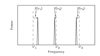
Figure 3: Schematic illustration of the frequency scatter due to a finite mode lifetime. Dashed lines are the true mode frequencies (Eq. 1), and solid peaks are measured frequencies.

In Fig. 3 we illustrate this by showing, schematically, the comb pattern of ‘true’ mode frequencies (dashed lines; Eq. 1) and the measured frequencies (solid peaks). The deviations, indicated with $X(\nu_{i})$ (Eq. 2), are independent because each mode is excited independently. Shorter mode lifetimes will give larger deviations. Following Bedding et al. (2004) and Kjeldsen et al. (2005), we estimate the mode lifetime from the scatter of the measured frequencies about a regular pattern. Our method differs by using a comb pattern for the reference frequencies, and by not requiring us to assign the mode order or degree to the measured frequencies. This is an advantage when the power spectrum is crowded due to aliasing and noise, as in this case, but the drawback is lower sensitivity to the mode lifetime.

The first step is to find the comb pattern that best matches our measured frequencies, $\nu\equiv[\nu_{1},\dots,\nu_{\mathrm{N}}]$. We do this by minimizing the RMS difference between the measured frequencies and those given by Eq. 1, with $\Delta\nu_{0}$ and $X_{0}$ as free parameters. The individual deviations are

$$X(\nu_{i})\equiv(\nu_{i}-X_{0})\bmod\Delta\nu_{0}\,,$$ (2)

where we use a modulo operator that returns values between $-\frac{1}{2}\Delta\nu_{0}$ and $\frac{1}{2}\Delta\nu_{0}$. The RMS scatter of $X$ is then

$$\sigma_{X}(\nu;\Delta\nu_{0},X_{0})=\frac{\sqrt{2}}{\Delta\nu_{0}}\sqrt{\frac{1}{N}\sum_{i=1}^{N}X(\nu_{i})^{2}}\,.$$ (3)

Here, $N=10$ is the number of frequencies. The normalization factor,$\sqrt{2}/\Delta\nu_{0}$, is included to make $\sigma_{X}$ independent of $\Delta\nu_{0}$ for randomly distributed frequencies. We find the minimum of $\sigma_{X}$, min($\sigma_{X}$), using the Amoeba minimization method (Press et al. 1992), and calibrate it against simulations with known mode lifetime, as described in the next section. As a by-product, we also get estimates for $\Delta\nu_{0}$ and $X_{0}$.

3.2 Simulations and calibration

We simulated the $\xi\,$Hya time series using the method described in Paper I. The oscillation mode lifetime was an adjustable parameter, assumed to be independent of frequency, while the other inputs for the simulator were fixed and chosen to reproduce the observations (see Paper I, Fig. 12). To make the simulations as realistic as possible, the input frequencies were the radial modes from a pulsation model of $\xi\,$Hya (Teixeira et al. 2003; Christensen-Dalsgaard 2004). Since our model assumes the frequencies to be strictly regular (Eq. 3), the intrinsic deviation of the input frequencies from a comb pattern (see Fig. 4) will contribute to $\sigma_{X}$. However, as described in Sect. 3.3, this contribution turns out to be negligible and therefore does not affect our measurement of the mode lifetime in $\xi\,$Hya.

Figure 4: Deviation of input frequencies from a comb pattern (Eq. 2).

For different values of the mode lifetime, we simulated 100 time series with different random number seeds. For each we measured 10 frequencies ($\nu_{1},\dots,\nu_{\mathrm{10}}$) using iterative sine-wave fitting (see Appendix A) and then minimized $\sigma_{X}$. This provided 100 values of min($\sigma_{X})$ for each mode lifetime, which can be compared with the observations. In Figs. 5 and 6 we illustrate the method, and Figs. 7 and 8 show the results. Fig. 5 shows $X(\nu_{i})$ of all 1000 frequencies (10 frequencies from each of 100 simulated time series) for two mode lifetimes, (a) $\tau=17$ days, and (b) $\tau=2$ days. The difference in mode lifetime is clearly reflected in the difference in the scatter of $X(\nu_{i})$. We note that the distribution of $X(\nu_{i})$ (right panels) is affected by the presence of false detections of alias peaks from neighbouring modes at roughly $X(\nu_{i})\sim 2\,\mu$Hz and $-2\,\mu$Hz (see Fig. 5a).

Figure 5: The deviation from a comb pattern (Eq. 2) for 10 measured frequencies from each of 100 simulated time series. The two horizontal bands (at $X(\nu_{i})\sim 2\,\mu$Hz and $-2\,\mu$Hz, most evident in panel (a)) below and above the central band are signatures of the alias peaks that are present in our spectral window (see Fig. 2). To the right, the distributions are shown for each panel.

In Fig. 6 we show $\sigma_{X}(\nu;\Delta\nu_{0},X_{0})$ for the case of $\tau=17\,$days. To smooth the plotted surface we show the average of all 100 simulations. However, during the minimization of $\sigma_{X}$, each simulations was treated separately.

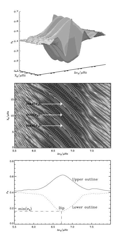
Figure 6: Top panel: 3D surface of $\sigma_{X}$, (averaged from 100 simulations with $\tau=17\,$days) as a function of the free parameters $X_{0}$ (plot range 0,20) and $\Delta\nu_{0}$ (plot range 5.5,8.0). Middle panel: The surface of $\sigma_{X}$ viewed from above, where contours are plotted to guide the eye. Solid lines indicate contours above the mean level, while the dotted lines are those below. Bottom panel: The outline of the 3D surface viewed edge on in the $X_{0}$-direction. The two output parameters of the minimization process, min($\sigma_{X}$) and the corresponding $\Delta\nu_{0}$, are indicated by dashed lines.

Note that $\sigma_{X}(\nu;\Delta\nu_{0},X_{0})=\sigma_{X}(\nu;\Delta\nu_{0},X_{0}+n\Delta\nu_{0})$, where $n$ is an integer, and that $\sigma_{X}$ has maxima and minima for roughly the same $\Delta\nu_{0}$ that are separated by $\frac{1}{2}\Delta\nu_{0}$ on the $X_{0}$-axis.

The output parameters min($\sigma_{X}$) and $\Delta\nu_{0}$ are plotted in Fig. 7.

Figure 7: Output from our method applied on 100 simulations of $\xi\,$Hya with mode lifetime 2 days (diamonds), and 17 days (plus symbols). The square shows the observational point, and the size of the symbol indicates the uncertainty according to the chosen CLEAN algorithm (cf. Sect. 3.3).

We see clearly that a smaller min($\sigma_{X}$) (more prominent comb pattern) gives a more accurate $\Delta\nu_{0}$ determination. In the case of short mode lifetime, the frequency pattern is generally not very pronounced (high min($\sigma_{X}$)) mainly due to the false detections from alias peaks.

Due to the stochastic variations in the simulated time series, the value of min($\sigma_{X}$) (Fig. 7) shows a large intrinsic scatter from one simulation to the next. This tells us the precision with which we can determine the mode lifetime, $\tau$, from a single data set. For each $\tau$, we compared the observed min($\sigma_{X}$) with the distribution from 100 independent simulations. This gives a measure of whether the observed value is consistent with $\tau$.

Figure 8: Distribution of the minimized scatter, $\sigma_{X}$, based on 10 frequencies from each of 100 simulations with different mode lifetimes: 17 days, 5 days, 2 days, and 6 hours. The dashed line indicates the value from the observations, and the vertical arrows show the median.

Fig. 8 shows the distributions of min($\sigma_{X}$) for simulations as histogram-plots, for different mode lifetimes ($\tau=17\,$days, $5\,$days, $2\,$days, and $6\,$hours). The dashed line indicates the observed value. For a mode lifetime of 17 days (corresponding to the damping rate in cyclic frequency, plotted by Houdek & Gough 2002, of $0.1\,\mu$Hz) only a few out of 100 trials have a value for min($\sigma_{X}$) as high as the observations.

The exact number depends on the exact choice of analysis method (see Sect. 3.3). We find the best match with observations for mode lifetimes of about 2 days, in good agreement with Paper I. However, we note that there is also a reasonable match for all mode lifetimes less than a day, as their distributions all look very similar to the bottom panel. Randomly distributed peaks also show similar distributions to $\tau=6\,$hours. Hence, if the mode lifetime of $\xi\,$Hya is only a fraction of a day it would definitely destroy any prospects for asteroseismology on this star. We have confirmed this with simulations that do not include any comb patterns by simulating a single mode with a mode lifetime of 2 hours, similar noise, excess power hump, and with the same total power as the above simulations.

3.3 Robustness of method

An important step for a correct interpretation of the results shown in Fig. 8 is to test the robustness of our method. We tested the dependence of the two relevant output parameters $\Delta\nu_{0}$ and min($\sigma_{X}$) on the following:

1. the initial guesses of $\Delta\nu_{0}$ and $X_{0}$ in the minimization process of $\sigma_{X}$,

2. the number of frequencies used to calculate $\sigma_{X}$,

3. whether weighting of frequencies is used when calculating $\sigma_{X}$,

4. the frequency separation of input frequencies,

5. the intrinsic scatter of input frequencies,

6. the method for measuring frequencies.

We discuss each of these in turn in Appendix B, but in summary, none of the listed points (1–6) have a significant effect on the results shown in Fig. 8.

4 Power and frequency analysis

To further investigate the mode lifetime for $\xi\,$Hya, we compared the observed cumulative distribution of the power spectrum from 1–190$\,\mu$Hz with that from simulations (Fig. 9). Note that the simulator is normalized so that on average it reproduces the observed power regardless of the mode lifetime (Paper I, Eq. 7). For each level in power, we calculated the fraction of the power spectrum that is above that level (similar to Fig. 2 in Delache & Scherrer 1983; see also Brown et al. 1991; Bedding et al. 2005b; Bruntt et al. 2005). We see only few time series of $\tau=17\,$days that have a power distribution similar to that observed and on average the difference is significant, while the distributions for $\tau=2\,$days resemble the observations much better. We note that there is a large intrinsic variation seen in the power distributions for $\tau=17\,$days.

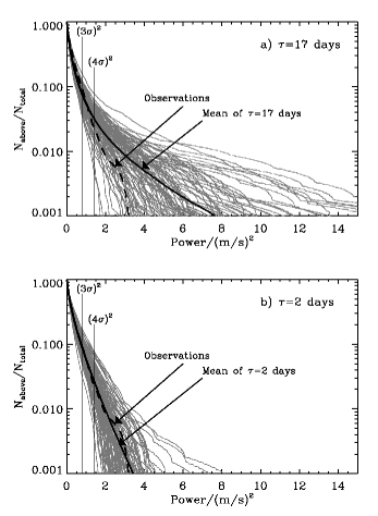
Figure 9: Panel (a): Cumulative distribution of power spectra from 100 simulations with $\tau=17\,$days (grey lines). The average distribution is shown with a black line. The dashed line indicates the distribution from the observations. Panel (b): Similar to panel (a), but with $\tau=2\,$days. The noise level in the observed power spectrum is indicated.

We also investigated the reliability of the observed frequencies (Table 1), using the simulations described in Sect. 3.2. The measured frequencies, together with the input frequencies and noise level are plotted in Fig. 10. Apart from the broadening of the mode frequencies due to damping, we also see false detections of alias peaks. This is most easily seen in panel (a) where the damping is less (a few examples of false detections are indicated). Our test shows that frequencies are not unambiguous if S/N$\lesssim$7–8, even for mode lifetimes of 17 days. For short mode lifetimes it looks rather hopeless to measure the individual mode frequencies with useful accuracy. The observed frequencies are all with S/N$<$6.3 and hence cannot be claimed to be unambiguous. Hence the frequencies in Table 1 (see also Fig. 10 bottom panel) should not be used for a direct comparison with individual frequencies from a pulsation model.

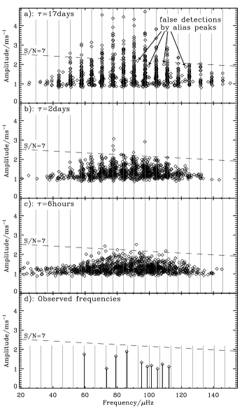
Figure 10: Each panel shows 1000 measured frequencies and their amplitudes (10 from each of 100 simulations). Dashed lines indicate 7 times the input noise, and the solid grey lines are the input frequencies. Panel (a): Mode lifetime = 17 days. Panel (b): Mode lifetime = 2 days. Panel (c): Mode lifetime = 6 hours. Panel (d): Observed frequencies and the best matching comb pattern (grey lines).

The lack of a clear comb pattern similar to Fig. 10 (top panel) in the observed frequencies also supports a short mode lifetime.

5 Discussion and future prospects

Our best match for the mode lifetime of $\xi\,$Hya ($\tau\sim 2\,$days) is in good agreement with our estimate in Paper I but disagrees with theory (Houdek & Gough 2002). This discrepancy indicates that red giants could be used to better understand the mechanisms of the driving and damping of oscillations in a convective environment. The short mode lifetime of $\xi\,$Hya also suggests a narrow range of mode lifetimes for a large range of stars, from the main sequence to the red giants, and hence a steep decline in the ‘quality’ factor (Fig. 1). The transition from the short mode lifetime regime to the much longer lifetimes of the semi-regular variables still needs to be investigated. It is likely to involve some kind of interaction between pure stochastic excitation and excitation by the $\kappa$ mechanism, which is responsible for the oscillations we see in Mira stars (Bedding 2003).

A difficulty in using the current observations of $\xi\,$Hya for asteroseismology arises from the severe crowding in the power spectrum. We now discuss possible origins of the crowding and some aspects of this issue.

We do not expect crowding from high amplitude non-radial modes in the power spectrum although low amplitude modes cannot be excluded (Christensen-Dalsgaard 2004, Paper I). Additional simulations are needed to quantify the effect on the lifetime estimate from low amplitude non-radial modes, but we expect it to be small.

The crowding in the power spectrum comes partly from the single-site spectral window, which emphasizes the importance of using more continuous data sets from multi-site campaigns or space missions. To illustrate this, we construct the combined time series from a hypothetical two-site observing campaign on $\xi\,$Hya where the observing window from each site is identical to that of the present data set obtained with the Coralie spectrograph. The other site is assumed to be a twin at the complementary longitude (12 hour time shift), and the two individual data sets have identical sampling and noise. We simulated the stellar signal using $\tau=2\,$days, with other parameters the same as for Fig. 12 in Paper I. A power spectrum of such a two-site time series is shown in Fig. 11. Each mode profile is seen much more clearly, though slightly blended due to the short mode lifetime. Obviously, more can be obtained from such a spectrum than from our present data set (Fig. 2), but a thorough analysis of similar simulations should be done to determine the prospects for doing asteroseismology on $\xi\,$Hya.

Figure 11: Power spectrum of simulated time series of $\xi\,$Hya ($\tau=2\,$days) using a window function from a two-site campaign where the sites are separated by 12 hours in longitude (see text). Dotted lines indicate the input frequencies.

As more high-quality asteroseismic data become available, simulations will continue to be an important tool for interpreting the data. However, one has to be careful about what can be deduced from simulations. Even though we may think, from an ideal perspective, that some parameters do not affect our measurements, this may turn out not to be true. A realistic noise source, the right window function, number- and scatter of frequencies, their amplitude and mode lifetime are all parameters that have to be considered when simulating oscillation data. Our comparison of the results from simplified simulations with more comprehensive simulations shows clearly that using simplified simulations can lead to erroneous conclusions. As an example, we measured an increase by a factor of two of min($\sigma_{X}$) between simulations including only 1 and 18 input frequencies. This demonstrates that it is important to use realistic (non-simplified) simulations to relate frequency scatter to the mode lifetime.

A complete application of our method on other stars (e.g. $\alpha\,$Cen A, $\nu\,$Ind, $\eta\,$Boo, and the Sun) will be published in a forthcoming paper.

6 Conclusions

We introduced a new method that uses only the scatter of the measured frequencies from a comb pattern to measure the mode lifetime of the red giant $\xi\,$Hya. This method takes into account false detections of noise and alias peaks. We find that the most likely mode lifetime is about 2 days, and we show that the theoretical prediction of 17 days (Houdek & Gough 2002) is unlikely to be the true value.

Due to the high level of crowding in the power spectrum, the signature from the p-modes is too weak to determine the large separation to very high accuracy. However, our measurement supports the separation of $6.8\,\mu$Hz found by Frandsen et al. (2002).

We conclude that the only quantities we can reliably obtain from the power spectrum of $\xi\,$Hya are the mode amplitude, mean mode lifetime, and the average large frequency separation.

Our simulations show that none of the measured frequencies from the $\xi\,$Hya data set (Frandsen et al. 2002) can be regarded as unambiguous. Hence we suggest the measured frequencies given in Table 1 are not used for direct mode-matching with a pulsation model to constrain the stellar model. Only in the case of a greatly improved window function could this be possible.

Appendix A CLEAN test

The method described in Sect. 3 required extraction of many frequencies. We therefore tested two different sine-wave fitting or CLEANing methods, simple CLEAN and CLEAN by simultaneous fitting. We call them CLEAN1 and CLEAN2, respectively. The tests were done on our simulated time series to gain better understanding of the results from CLEANing and to determine which method was most favorable in our case. Both methods subtract one frequency at a time (the one with highest amplitude), but CLEAN2 recalculates the parameters (amplitude, phases, and frequencies) of the previously subtracted peaks while fixing the frequency of the latest extracted peak. In this way, the fit of the sinusoids to the time series is done simultaneously for all peaks. CLEAN1, however, does not recalculate the parameters of previously subtracted peaks. The time used by CLEAN2 is a factor of $1.5(N_{\mathrm{extract}}+1)$ longer than for CLEAN1, where $N_{\mathrm{extract}}$ is the number of extracted frequencies.

We made simulations similar to those described in Sect. 3.2 but with 17 equally spaced frequencies and no noise added. From each set of 100 time series with a given mode lifetime, 10 frequencies were extracted providing 1000 frequencies which we compared with the input frequencies. For coherent oscillations CLEAN2 is doing a perfect job while CLEAN1 detected 1% false peaks. If only true detections are considered, the scatter of the extracted frequencies relative to the input is roughly equal to the frequency resolution ($1/T_{\mathrm{obs}}$) for CLEAN2, while the CLEAN1 results scatter twice as much.

For non-coherent oscillations, the number of false detections increases for both methods and the relative success rates of the two methods become equally good (or bad), for mode lifetimes in the order of the observational window or shorter. In this regime, the scatter of the extracted frequencies gets dominated by the mode damping and is independent of the CLEANing method. For mode lifetimes below 5 days, the scatter of the frequencies is so pronounced relative to the spacing between modes and the alias peaks that they overlap and it cannot be determined whether an extracted frequency is false or not (see e.g. Fig. 5b).

The amplitude of a detected frequency found by both CLEANing methods generally differ by maximum +/-30% but can for a few cases differ by 70%, being most severe for shorter mode lifetimes. There is a general trend that CLEAN2 ascribes lower amplitudes to the peaks of highest amplitude in a spectrum, and higher amplitudes to low amplitude peaks relative to CLEAN1. This is a result of the recalculation of the oscillation parameters in CLEAN2. The detected amplitude difference was not considered as crucial as we were interested in using the frequencies only. Since there is observational evidence that the mode lifetime of $\xi\,$Hya is below 5 days (Paper I), where the two methods perform equally well, we choose CLEAN1 due to its faster algorithm (by a factor of 17 in our case where $N_{\mathrm{extract}}=10$).

Appendix B Robustness tests

In this appendix we discuss each of the points (1–6) listed in Sect. 3.3 in turn:

(1) In the minimization process, the initial guesses of $\Delta\nu_{0}$ and $X_{0}$ could give quite different outputs for $\Delta\nu_{0}$ on a data set with a shallow dip in $\sigma_{X}$ (i.e weak comb pattern). For data with a deep dip in $\sigma_{X}$ (i.e. strong comb pattern), $\Delta\nu_{0}$ is unaffected. We found that min($\sigma_{X}$) was well determined if the initial guess of $\Delta\nu_{0}$ was within $\sim 1\,\mu$Hz of the true value. As a representative example we see $\pm 1.5\,\mu$Hz change in $\Delta\nu_{0}$ and only $\pm 0.008\,\mu$Hz change in min($\sigma_{X}$) for the set of observed frequencies, which produced a shallow dip in min($\sigma_{X}$). Our final setup (plotted in Fig. 8) was to fix the initial guess of $\Delta\nu_{0}$ at $6.8\,\mu$Hz, which we believe is within $1\,\mu$Hz of the true value, and to use 7 different $X_{0}$ values (separated $1\,\mu$Hz apart). We then chose the solution with the lowest minimum found from these 7 trials.

(2) We investigated the changes in the output parameters (min($\sigma_{X}$), $\Delta\nu_{0}$), from varying the number of measured frequencies from 5 to 10. The average $\Delta\nu_{0}$ is unaffected by the number of frequencies, but more frequencies give a more accurate $\Delta\nu_{0}$ determination. For the observed frequencies $\Delta\nu_{0}$ changes by $\pm 0.5\,\mu$Hz in the tested regime (from 5 to 10 frequencies). Furthermore we observed higher values of min($\sigma_{X}$), thus weaker comb patterns, with increasing number of frequencies, but the relative difference between the min($\sigma_{X}$) distributions from simulations and the observational data point did not change significantly.

We decided to use 10 frequencies since we trusted our min($\sigma_{X}$) distributions more when the $\Delta\nu_{0}$ determinations were closer to the true value. Measuring more than 10 frequencies showed no clear advantage, for this particular data set.

(3) Assigning weights to each frequency according to its S/N makes the absolute value of min($\sigma_{X}$) slightly less sensitive to the number of measured frequencies used to calculate min($\sigma_{X}$), which is expected. Due to the higher weight given to the central part of the damping profile for each mode (Anderson et al. 1990), the frequency separation is also slightly better determined using weights. However, min($\sigma_{X}$) will scatter slightly more, making it more difficult to distinguish min($\sigma_{X}$) distributions from different mode lifetimes. This is probably a result of assigning lower weight to the tails of the damping profile. We chose not to use weights, to obtain the best possible result on the mode lifetime.

(4) Changing the large separation of the input frequencies did not produce any change in min($\sigma_{X}$) for the tested range (6.8–7.2$\,\mu$Hz), but only changed the output $\Delta\nu_{0}$ accordingly. Hence, it is not crucial for our results on the mode lifetime to know the true frequency separation to a very high accuracy.

(5) We also changed the deviation, $X(\nu_{i})$, from a comb pattern of the input frequencies. We used input frequencies that had a deviation twice as large as in the pulsation model (see Fig. 4), and also a frequency set that followed a perfectly regular comb. No significant change of the min($\sigma_{X}$) distributions (Fig. 8) was observed. We believe this is because min($\sigma_{X}$) is dominated by damping for the mode lifetimes we investigated.

(6) Finally, we investigated whether the choice of frequency extraction method affects min($\sigma_{X}$) and $\Delta\nu_{0}$. Using three different algorithms on the observations provided 3 different sets of measured frequencies, and hence 3 different min($\sigma_{X}$) values that ranged from 0.23–0.28. The corresponding output $\Delta\nu_{0}$ ranged from 6.7–7.2$\,\mu$Hz. We note, that the min($\sigma_{X}$) distributions seen in Fig. 8 did not change significantly.

References

- Anderson et al. (1990) Anderson, E. R., Duvall, T. L., & Jefferies, S. M. 1990, ApJ, 364, 699
- Bedding et al. (2003) Bedding, T., Kiss, L., & Kjeldsen, H. 2003, Solar and Solar-Like Oscillations: Insights and Challenges for the Sun and Stars, 25th meeting of the IAU, Joint Discussion 12, 18 July 2003, Sydney, Australia, 12
- Bedding (2003) Bedding, T. R. 2003, Ap&SS, 284, 61
- Bedding et al. (2005a) Bedding, T. R., Kiss, L. L., Kjeldsen, H., et al. 2005a, MNRAS, 361, 1375
- Bedding et al. (2005b) Bedding, T. R., Kjeldsen, H., Bouchy, F., et al. 2005b, A&A, 432, L43
- Bedding et al. (2004) Bedding, T. R., Kjeldsen, H., Butler, R. P., et al. 2004, ApJ, 614, 380
- Brown et al. (1991) Brown, T. M., Gilliland, R. L., Noyes, R. W., & Ramsey, L. W. 1991, ApJ, 368, 599
- Bruntt et al. (2005) Bruntt, H., Kjeldsen, H., Buzasi, D. L., & Bedding, T. R. 2005, ApJ, 633, 440
- Buzasi et al. (2000) Buzasi, D., Catanzarite, J., Laher, R., et al. 2000, ApJ, 532, L133
- Chaplin et al. (1997) Chaplin, W. J., Elsworth, Y., Isaak, G. R., et al. 1997, MNRAS, 288, 623
- Christensen-Dalsgaard (2004) Christensen-Dalsgaard, J. 2004, Sol. Phys., 220, 137
- Christensen-Dalsgaard et al. (2001) Christensen-Dalsgaard, J., Kjeldsen, H., & Mattei, J. A. 2001, ApJ, 562, L141
- Delache & Scherrer (1983) Delache, P. & Scherrer, P. H. 1983, Nature, 306, 651
- Dind (2004) Dind, Z. E. 2004, Mode Lifetimes in Semi-Regular Variables, Honours thesis, School of Physics, University of Sydney
- Dziembowski et al. (2001) Dziembowski, W. A., Gough, D. O., Houdek, G., & Sienkiewicz, R. 2001, MNRAS, 328, 601
- Frandsen et al. (2002) Frandsen, S., Carrier, F., Aerts, C., et al. 2002, A&A, 394, L5
- Guenther et al. (2000) Guenther, D. B., Demarque, P., Buzasi, D., et al. 2000, ApJ, 530, L45
- Houdek et al. (1999) Houdek, G., Balmforth, N. J., Christensen-Dalsgaard, J., & Gough, D. O. 1999, A&A, 351, 582
- Houdek & Gough (2002) Houdek, G. & Gough, D. O. 2002, MNRAS, 336, L65
- Kiss & Bedding (2003) Kiss, L. L. & Bedding, T. R. 2003, MNRAS, 343, L79
- Kjeldsen (2003) Kjeldsen, H. 2003, Ap&SS, 284, 1
- Kjeldsen et al. (2005) Kjeldsen, H., Bedding, T. R., Butler, R. P., et al. 2005, ApJ, accepted
- Libbrecht (1988) Libbrecht, K. G. 1988, ApJ, 334, 510
- Montgomery & O’Donoghue (1999) Montgomery, M. H. & O’Donoghue, D. 1999, Delta Scuti Star Newsletter 13, 28 (University of Vienna)
- Press et al. (1992) Press, W. H., Teukolsky, S. A., Vetterling, W. T., & Flannery, B. P. 1992, Numerical recipes in C. The art of scientific computing (Cambridge: University Press, —c1992, 2nd ed.)
- Retter et al. (2003) Retter, A., Bedding, T. R., Buzasi, D. L., Kjeldsen, H., & Kiss, L. L. 2003, ApJ, 591, L151, erratum: 596, L125
- Samadi et al. (2004) Samadi, R., Goupil, M. J., Baudin, F., et al. 2004, in ESA SP-559: SOHO 14 Helio- and Asteroseismology: Towards a Golden Future, 615
- Stello (2002) Stello, D. 2002, Master’s thesis, Institut for Fysik og Astronomi, Aarhus Universitet, available HTTP: http:www.phys.au.dkstelloPublicationsthesis.pdf
- Stello et al. (2004) Stello, D., Kjeldsen, H., Bedding, T. R., et al. 2004, Sol. Phys., 220, 207
- Teixeira et al. (2003) Teixeira, T. C., Christensen-Dalsgaard, J., Carrier, F., et al. 2003, Ap&SS, 284, 233
- Thévenin et al. (2005) Thévenin, F., Kervella, P., Pichon, B., et al. 2005, A&A, 436, 253