Computation of Fluid Flows in Non-inertial Contracting, Expanding, and Rotating Reference Frames

Abstract

We present the method for computation of fluid flows that are characterized by the large degree of expansion/contraction and in which the fluid velocity is dominated by the bulk component associated with the expansion/contraction and/or rotation of the flow. We consider the formulation of Euler equations of fluid dynamics in a homologously expanding/contracting and/or rotating reference frame. The frame motion is adjusted to minimize local fluid velocities. Such approach allows to accommodate very efficiently large degrees of change in the flow extent. Moreover, by excluding the contribution of the bulk flow to the total energy the method eliminates the high Mach number problem in the flows of interest. An important practical advantage of the method is that it can be easily implemented with virtually any implicit or explicit Eulerian hydrodynamic scheme and adaptive mesh refinement (AMR) strategy.

We also consider in detail equation invariance and existence of conservative formulation of equations for special classes of expanding/contracting reference frames. Special emphasis is placed on extensive numerical testing of the method for a variety of reference frame motions, which are representative of the realistic applications of the method. We study accuracy, conservativity, and convergence properties of the method both in problems which are not its optimal applications as well as in systems in which the use of this method is maximally beneficial. Such detailed investigation of the numerical solution behavior is used to define the requirements that need to be considered in devising problem-specific fluid motion feedback mechanisms.

,

1 Introduction

Many fluid dynamical problems, particularly the ones of high importance in astrophysics and cosmology, have the following two key characteristics: (1) the fluid undergoes a very large degree of expansion/contraction on its evolutionary timescale; (2) the flow consists of the global component, associated with the overall expansion/contraction and, if present, rotation of the system and the superimposed local fluid velocity field, with the global flow velocity being much larger than the local fluid velocity or the local sound speed. Additionally, such systems are often characterized by the linear distribution of total velocity along the radius, sometimes referred to as the Hubble flow by analogy with cosmology. Astrophysical examples include, but are not limited to, stellar core collapse, supernova explosions (SNe), star and galaxy formation, as well as cosmological models. One of the most prominent examples of such systems in terrestrial applications is the inertial confinement fusion (ICF) problem. Compression or expansion of matter in those problems may reach many orders of magnitude.

Problems with large degree of expansion/contraction are computationally difficult. Local features of the flow in those problems are significantly compressed, expanded, and advected over large distances. This puts extreme demands on numerical resolution and on the quality of numerical advection algorithms. For the rotating fluid large compression or expansion may also lead to large numerical errors in conservation of angular momentum.

Three different approaches in the context of Eulerian formalism can be used to overcome some of those computational difficulties: (1) adaptive mesh refinement (AMR), (2) computations on a moving mesh (MM), and (3) computations in a moving (non-inertial) reference frame (MRF). The first two approaches are being widely used to address the first characteristic of the flows, mentioned above, namely to accommodate large degrees of flow expansion or contraction. In an AMR approach (e.g., see [1, 11]), the computational mesh is refined or derefined to counteract respectively flow contraction or expansion thus maintaining numerical resolution of the features of interest. One representative example is the AMR calculation of star formation in the early Universe (see [10] and references therein). As opposed to increasing or decreasing the number of cells following the flow in the AMR approach, in the MM techniques mesh lines are moved continuously to minimize the relative motion of the fluid with respect to the computational grid [2, 3, 4] thereby providing expansion or contraction of the grid in accordance with the motion of the flow. This general method also includes a large class of techniques referred to as arbitrary Lagrangian-Eulerian method (ALE) [5, 6] in which the mesh is deformed to follow the fluid flow. A recent astrophysical example is the use of a traditional moving mesh technique [3] to follow explosion of a type Ia SNe to the stage of free ballistic expansion [7, 8].

The AMR and MM approaches are fundamentally similar in that they both work with fluid quantities defined in a stationary inertial reference frame. The only difference is that in the AMR approach the fluid moves through a stationary mesh and an additional interpolation is required only when the mesh is refined or derefined. In the MM approach coordinate transformation between the physical space and the computational domain is provided and at every time step the formal correspondence (transformation map) between computational and physical coordinates is established. Thus fluid quantities must be re-interpolated onto a new mesh every time step either explicitly via an Eulerian step plus re-map, or implicitly by modifying fluxes through boundaries of computational cells. Since fluid variables are defined in a stationary frame they are not affected by mesh movements. While the AMR and MM approaches are capable of addressing the first characteristic of the flows discussed above, this key property of those methods makes them inefficient in modeling flows dominated by the global component associated with expansion/contraction and/or rotation. In such systems practically all of the kinetic energy is due to the global flow, thus the ratio of thermal to kinetic energy can be extremely small. Consequently, solving for the total energy in the inertial reference frame results in large errors in thermal energy and, thus, pressure. This situation is well known in hydrodynamics as a high Mach number problem and various methods have been employed to solve it in different contexts (e.g., see [9] and references therein).

The goal of the MRF approach is to address that problem while preserving the efficiency of the MM method in accommodating large degrees of the flow expansion/contraction. In the MRF method the full reference frame transformation is performed, as opposed to only the coordinate transformation in the MM approaches. Fluid velocities and total energy are defined with respect to a comoving reference frame in which thermal and local kinetic energies are comparable in magnitude thereby eliminating the high Mach number problem. Computational mesh in this approach has two distinct functions. It defines the boundaries of computational cells and, at the same time, represents a reference frame. Consequently, the equations of fluid dynamics must be modified to include the effects of frame expansion, acceleration, as well as forces arising due to the reference frame rotation.

The area of widest use of the MRF approach in astrophysics, albeit in a somewhat simplified sense, are cosmological simulations. In those simulations the terms accounting for expansion of the Universe are known a priori and are explicitly added as source terms to the fluid equations [10]. In [9] a collapse of a cosmological pancake was considered in a non-inertial reference frame the motion of which was implicitly defined by self-gravity of the pancake structure itself. It is impossible to pick a single ”best” numerical approach to solving all fluid dynamics problems. The right choice must depend on the problem in question and often it is a compromise between accuracy, flexibility, ease of applicability, and code availability. The approaches discussed above can be and are often used in combination. For example, simulations of galaxy formation routinely combine a MRF approach which accounts for global expansion of the Universe with the AMR or MM approaches used for a more accurate treatment of structure formation on smaller scales.

In this paper we investigate the applicability of the MRF approach and its combination with AMR to astrophysical problems involving expanding / contracting and rotating objects such as collapsing stellar cores and supernovae. Such systems exhibit the two key characteristics discussed above. We also have in mind applications to implosion of ICF targets ablated by laser radiation.

We consider non-inertial reference frames which expand or contract spherically-symmetrically with respect to an inertial laboratory frame. A solid (non-differential) rotation of the frame is also allowed. In many practical cases this may be enough to compensate for the bulk motion associated with the explosion of a star or implosion of an ICF target. We work on a premise that peculiar motions, local deformations, and sharp features, e.g., shocks, contact and material discontinuities, and reaction fronts, present in the flow can be better treated using the AMR method applied in a moving frame. Our goal in this work is to investigate general numerical properties of the method which involves computations in such a non-inertial reference frame. In particular, our emphasis is on the accuracy, conservativity, and convergence properties of the method under different types of reference frame motions. Such properties can then be used in devising problem-specific feedback mechanisms that define specific reference frame motions based on the fluid flow evolution.

In § 2 we discuss the general transformation to the moving non-inertial reference frame of the type discussed above, we write down the transformed set of fluid equations and we also discuss the invariance of the original equations and the existence of conservative formulation. In § 3 we discuss the numerical method used in solving the transformed set of fluid equations. In § 4 we present results of numerical tests. We use two completely independent AMR codes - ALLA and AstroBEAR [11, 12], which differ in their hydrodynamic integration schemes and in their AMR approach (cell-based vs. grid- or patch-based). The testing is twofold. On one hand, we present a series of tests which are not the optimal applications of this method and which are designed to stress the method. They include the strong point explosion (Sedov blast wave) and the converging shock (Guderley blast wave). However, those tests give a very good idea of the limitations of the MRF method which must be always kept in mind while using the MRF approach in real applications. We also consider a series of tests for which this method is extremely well suited. Those tests are based on the expansion of a non-rotating and a rotating sphere into vacuum and isentropic expansion of a uniform pressure field with embedded density structure. Discussion and conclusions are given in § 5, where we also discuss performance comparison of the method presented here and the moving mesh approach using as an example the moving mesh implementation of the Zeus-MP code [13]. Finally, Appendix A presents the special case of transformed fluid equations in cylindrical coordinates in the absence of rotation.

2 Equations of Fluid Dynamics in an Expanding/Contracting and Rotating Reference Frame

2.1 General formalism

We start with an inertial Cartesian (laboratory) reference frame $\mathbf{X}=\{\mathbf{r},t\}$. Euler equations of fluid dynamics in this frame are

$${\partial{\rho}\over\partial{t}}+\nabla\cdot(\rho\mathbf{u}) \quad=\quad 0,$$ (1)

$${\partial{\rho\mathbf{u}}\over\partial{t}}+\nabla\cdot(\rho\mathbf{u}\otimes\mathbf{u})+\nabla P \quad=\quad 0,$$ (2)

$${\partial{E}\over\partial{t}}+\nabla\cdot\big{(}(E+P)\mathbf{u}\big{)} \quad=\quad 0,$$ (3)

where $\rho$ is mass density, $\mathbf{u}$ - fluid velocity, $P$ - pressure, $E=\rho\,e+\frac{1}{2}\rho u^{2}$ - energy density, and $e$ - internal energy per unit mass.

Next we consider a non-inertial reference frame $\mathbf{\tilde{X}}=\{\mathbf{\tilde{r}},\tau\}$, which rotates and homologously expands or contracts with respect to $\mathbf{X}$. The frame $\mathbf{\tilde{X}}$ is defined by the transformation $\mathbf{\Lambda}:\mathbf{X}\mapsto\mathbf{\tilde{X}}$

$$\mathbf{\Lambda}=\left\{\begin{array}[]{lcl}\mathbf{\tilde{r}}&=&\displaystyle a^{-1}\left(\mathbf{r}-\int_{0}^{t}\mathbf{\omega}(t)dt\times\mathbf{r}\right),\\ \tau&=&\displaystyle\int_{0}^{t}\frac{dt}{a^{\beta+1}},\end{array}\right.$$ (4)

where $\beta$ is a constant. We require the transformation $\mathbf{\Lambda}$ to be non-singular, therefore we assume that the scale factor $a(t)$ is a smooth non-vanishing twice-differentiable function of time only. Angular velocity of the frame $\mathbf{\omega}(t)$ is assumed to be a smooth once differentiable function of time. Here we consider only the cases of solid body rotation, i.e., the cases when $\mathbf{\omega}$ is only a function of time and not spatial coordinates, and we assume that $\mathbf{\omega}$ does not change its spatial orientation. Note, that $d\tau=dt/a^{\beta+1}$. The inverse transformation is

$$\mathbf{\Lambda}^{-1}=\left\{\begin{array}[]{lcl}\mathbf{r}&=&\displaystyle a(\tau)\left(\tilde{\mathbf{r}}-\int_{0}^{\tau}\mathbf{\Omega}(\tau)d\tau\times\tilde{\mathbf{r}}\right),\\ t&=&\displaystyle\int_{0}^{\tau}a^{\beta+1}(\tau)d\tau,\end{array}\right.$$ (5)

where we introduced the effective angular velocity

$$\mathbf{\Omega}=a^{\beta+1}\mathbf{\omega}=a^{\beta+1}\frac{d\mathbf{\phi}}{dt}=\frac{d\mathbf{\phi}}{d\tau},$$ (6)

which describes the angle swept by the reference frame $\mathbf{\tilde{X}}$ per unit computational time.

Hereafter, quantities with the tilde sign refer to the reference frame $\mathbf{\tilde{X}}$. For simplicity we will also be referring to the stationary laboratory frame $\mathbf{X}$ as the physical frame and to time $t$ as the physical time. Since typically in the numerical tests discussed below the computational grid is associated with the frame $\mathbf{\tilde{X}}$ we will be referring to this frame as the computational frame and to time $\tau$ as the computational time.

The transformation $\mathbf{\Lambda}$ implies the decomposition of the velocity field $\mathbf{u}$, present in the frame $\mathbf{X}$, into the sum of the bulk velocity associated with the global expansion/contraction and rotation, and the superimposed local velocity field $\mathbf{\tilde{u}}$ in the frame $\mathbf{\tilde{X}}$

$$\mathbf{u}=\mathbf{\Omega}\times\mathbf{\tilde{r}}+a^{-\beta}\frac{d\ln a}{d\tau}\mathbf{\tilde{r}}+a^{-\beta}\mathbf{\tilde{u}}.$$ (7)

Thus $\mathbf{\Lambda}$ provides a homologous spatial transformation ensuring that if matter expands/contracts spherically and rotates with velocity $\mathbf{u^{\prime}}=\mathbf{\omega}\times\mathbf{r}+H(t)\mathbf{r}$ in the stationary frame $\mathbf{X}$, then that matter will be at rest in the computational reference frame $\mathbf{\tilde{X}}$. The scale factor $a(t)$ can be defined by $\dot{a}(t)/a=H(t)$, where $\dot{a}$ is the derivative with respect to physical time and not the new transformed time $\tau$. Converting to $\tau$ we get

$$\dot{a}=\frac{da}{d\tau}\frac{d\tau}{dt}=\frac{1}{a^{\beta}}\frac{d\ln a}{d\tau}.$$ (8)

Similarly, we note another useful relation

$$\ddot{a}=\frac{d\dot{a}}{d\tau}\frac{d\tau}{dt}=\frac{1}{a^{2\beta+1}}\Bigg{\{}\frac{d^{2}\ln a}{d\tau^{2}}-\beta\left(\frac{d\ln a}{d\tau}\right)^{2}\Bigg{\}}.$$ (9)

Via the transformation $\mathbf{\Lambda}$ we, in effect, introduced the scaling of length and time. We have the third independent physical quantity, namely mass, the scaling of which we introduce via the density field

$$\tilde{\rho}(\tilde{\mathbf{r}},\tau)=a^{\alpha}\rho.$$ (10)

Here $\alpha$, as well as $\beta$ in (4), are the scaling parameters.

In the reference frame $\mathbf{\tilde{X}}$ the Euler equations (1) - (3) become

$${\partial{\tilde{\rho}}\over\partial{\tau}} \,+\, \tilde{\nabla}\cdot(\tilde{\rho}\,\mathbf{\tilde{u}})=\left(\alpha-\nu\right)\frac{d\ln a}{d\tau}\tilde{\rho},$$ (11)

$$\displaystyle{\partial{\tilde{\rho}\,\mathbf{\tilde{u}}}\over\partial{\tau}} \,+\, \tilde{\nabla}\cdot(\tilde{\rho}\,\mathbf{\tilde{u}}\otimes\mathbf{\tilde{u}})+\tilde{\nabla}\tilde{P}=(\alpha-\nu+\beta-1)\frac{d\ln a}{d\tau}\tilde{\rho}\,\mathbf{\tilde{u}}-$$ (12)

$$\displaystyle\Bigg{\{}\frac{d^{2}\ln a}{d\tau^{2}}-\beta\left(\frac{d\ln a}{d\tau}\right)^{2}\Bigg{\}}\tilde{\rho}\,\mathbf{\tilde{r}}-\tilde{\rho}\Bigg{[}\mathbf{\Omega}\times(\mathbf{\Omega}\times\mathbf{\tilde{r}})+$$

$$\displaystyle\left(\frac{d\ln\Omega}{d\tau}+\left(1-\beta\right)\frac{d\ln a}{d\tau}\right)\,\mathbf{\Omega}\times\mathbf{\tilde{r}}\Bigg{]}-2\mathbf{\Omega}\times\tilde{\rho}\mathbf{\tilde{u}},$$

$$\displaystyle{\partial{\tilde{E}}\over\partial{\tau}} \,+\, \tilde{\nabla}\cdot\bigg{(}\mathbf{\tilde{u}}\left(\tilde{E}+\tilde{P}\right)\bigg{)}=\frac{d\ln a}{d\tau}\bigg{[}\left(\alpha-\nu+2\beta\right)\tilde{E}-\nu\tilde{P}-\tilde{\rho}\tilde{u}^{2}\bigg{]}-$$ (13)

$$\displaystyle\Bigg{\{}\frac{d^{2}\ln a}{d\tau^{2}}-\beta\left(\frac{d\ln a}{d\tau}\right)^{2}\Bigg{\}}\left(\tilde{\rho}\mathbf{\tilde{u}}\cdot\mathbf{\tilde{r}}\right)-\left(\tilde{\rho}\mathbf{\tilde{u}}\cdot\mathbf{\Omega}\right)\left(\mathbf{\tilde{r}}\cdot\mathbf{\Omega}\right)+\Omega^{2}\left(\tilde{\rho}\mathbf{\tilde{u}}\cdot\mathbf{\tilde{r}}\right)-$$

$$\displaystyle\left(\frac{d\ln\Omega}{d\tau}+\left(1-\beta\right)\frac{d\ln a}{d\tau}\right)\tilde{\rho}\mathbf{\tilde{u}}\cdot\left(\mathbf{\Omega}\times\mathbf{\tilde{r}}\right),$$

where $\tilde{E}=\tilde{\rho}\tilde{e}+\frac{1}{2}\tilde{\rho}\tilde{u}^{2}$, and $\tilde{\nabla}$ indicates differentiation with respect to spatial coordinates $\mathbf{\tilde{r}}$. Hereafter, $\nu$ is the dimensionality parameter of the problem. The transformed pressure and internal energy fields have the form

$$\tilde{P}(\tilde{\mathbf{r}},\tau)=a^{\alpha+2\beta}P;\quad\tilde{e}(\tilde{\mathbf{r}},\tau)=a^{2\beta}e;$$ (14)

The first terms on the right-hand side of eqs. (11) - (13) are associated with expansion/contraction per se of the reference frame, while the second terms represent the effects of the frame acceleration. The remainder of the terms in eqs. (12) and (13) describe the effects of the frame rotation. In particular, the first term in square brackets in eq. (12) is the centrifugal force while the second term is related to the unsteadiness of the frame rotation and, finally, the last term on the right-hand side of the equation is the Coriolis force.

The only two parameter functions that have not been defined yet are the scale factor $a(t)$ and the angular velocity $\mathbf{\omega}(t)$. Typically, the choice of these functions is problem-specific and their temporal evolution is governed by fluid motions in the system. Thus a realistic application of the method presented here requires a feedback mechanism with appropriate filtering that will translate complex multidimensional fluid motions into smooth functions $a(t)$ and $\mathbf{\omega}(t)$. Since in this work we are primarily concerned with the general properties of the method we do not consider such feedback. Instead, we limit the discussion only to such types of computational frames the motion of which with respect to the inertial frame is predefined, e.g, via an analytic prescription. We chose a set of computational frames that covers a large range of possible motions and that is rather numerically challenging. This allows us to illustrate below accuracy, stability, and conservativity properties of our approach which can be later used in devising the problem-specific feedback filters.

The method presented here is naturally able to accommodate large degrees of expansion or contraction of fluid flows. However, as it was discussed in § 1, the second key characteristic of the flows, which we are interested in modeling, is the fact that the fluid velocity associated with the global flow due to its expansion/contraction and, if present, rotation greatly exceeds both the local peculiar velocities and the sound speed. In the context of eq. (7) this statement can be written as

$$|\tilde{\mathbf{u}}|\ll a^{\beta}|\mathbf{\omega}\times\mathbf{r^{*}}+H(t)\mathbf{r^{*}}|;\quad\tilde{c}\ll a^{\beta}|\mathbf{\omega}\times\mathbf{r^{*}}+H(t)\mathbf{r^{*}}|.$$ (15)

where $H(t)=\dot{a}(t)/a$ and $r^{*}$ defines the maximum extent of the flow, where the largest bulk flow velocities exist. Note that because of the relations (10) and (14) the local sound speed $c$ is transformed as $\tilde{c}=a^{\beta}c$. As an example, consider Fig. 6 representing the increase of kinetic energy in the case of expansion of a non-rotating and a rotating sphere into vacuum. We discuss these two tests in detail in § 4.2. As the sphere material is accelerated to its terminal expansion velocity, kinetic energy rapidly approaches total energy and then for more than 75% of the total simulation run time in the non-rotating case and more than 90% of the time in the rotating case it constitutes over 99% of the total energy. Practically all of that kinetic energy is associated with the global fluid flow. Thus in the inertial frame thermal component is only a small fraction of the total energy and solving for the latter would result in large errors in pressure and, consequently, the overall solution. On the other hand, in the computational frame $\mathbf{\tilde{X}}$, which closely follows global fluid motions, thermal and local kinetic energies are comparable in magnitude thereby eliminating the high Mach number problem and resulting in much smaller errors in pressure.

The method presented here is not equally efficient in treating all fluid flows that undergo substantial expansion/contraction in the course of their evolution and exhibit property (15). Consider shock strength $\Pi=\Delta P/\rho_{0}c^{2}_{0}$, where $\Delta P$ is pressure jump over the shock, $\rho_{0}$ is pre-shock fluid density and $c_{0}$ is pre-shock sound speed. It is an invariant of the transformation $\mathbf{\Lambda}$ and the associated transformations (10) and (14). In practice, consideration of such invariant quantities can define the extent of applicability of the method presented here and its efficiency in a given application. Next consider a problem involving propagation of the global shock into stationary medium, e.g., due to a strong point explosion. In a co-expanding frame $\mathbf{\tilde{X}}$, the velocity of which was adjusted to the shock speed, the shock will be stationary. However, its strength $\Pi$ must be maintained and that is achieved by the opposing velocity gradient $\mathbf{\tilde{u}}=-\dot{a}\mathbf{\tilde{r}}$, which is the direct result of the application of the velocity transformation (7) to the zero velocity field of the ambient material. In general, any regions of material, which is stationary in the inertial reference frame and which is dynamically important, will have such velocity gradients which may be quite large. This can limit the computational time step. Therefore, such problems do not constitute an optimal class of applications for this method. On the other hand, expanding or collapsing environments, in which ambient conditions are vacuous or dynamically unimportant so that the ambient fluid can be set to be stationary in the computational frame, or in which the computational domain contains the interior of the expanding or collapsing flow represent the class of applications most suited for this method. Finally, it is always advantageous to consider rapidly rotating flows in the co-rotating frame. Below we consider examples of both types of problems.

Finally, it should be noted that while the system (1) - (3), and consequently the transformed system (11) - (13), are the most general sets of equations, there are special cases, for example, employing specific symmetries of the problem at question, that may be of interest in various applications. One such case, namely the case of cylindrical symmetry, is considered in Appendix A. There may also be more general forms of the scale factor $a$ and the angular velocity of the frame $\mathbf{\omega}$ that may be useful. One important generalization is the scale factor that depends not only on time but also on radial distance $a(r,t)$. This would allow one to isolate certain regions of the domain that would be comoving with the global flow but that would not experience expansion and, therefore, would not suffer from the loss of numerical resolution in physical space. However, such transformations are outside the scope of this work.

2.2 Equation invariance and conservative formulation

The first important question that has to be answered regarding eqs. (11) - (13) is whether there exists their conservative formulation. Traditionally it is considered beneficial in the numerical hydrodynamics to work with the conservative formulation of Euler equations. In the moving mesh approach, which relies on the coordinate remapping instead of a true reference frame transformation, it is always possible for any coordinate transformation to cast Euler equations in a “conservative” form

$$\left(Jq\right)_{t}+\tilde{\nabla}\cdot\tilde{F}=0,$$ (16)

with a new vector of conserved quantities $q^{*}=Jq$, where $J$ is the Jacobian of the coordinate transformation, and some modified flux functions $\tilde{F}_{i}$. Indeed, primitive variable fields, including velocities which are always defined in the inertial frame $\mathbf{X}$, are not changed by the coordinate transformation. Therefore, the Hamiltonian structure of the system remains invariant. Consequently all conserved quantities are preserved and only their volumetric densities are affected due to the rescaling of length introduced by the coordinate transformation, which is reflected in the Jacobian factor. When the true reference frame, and not just coordinate, transformation is employed, e.g., the transformation $\mathbf{\Lambda}$, that immediately changes the structure of Action and the Hamiltonian of the system, which now attain some generally non-trivial explicit temporal dependence due to the functions $a(t)$ and $\mathbf{\omega(t)}$. In particular, the Hamiltonian in the frame $\mathbf{\tilde{X}}$ takes the form (see also [14])

$$\tilde{H} \,= \,\int\int\int d\mathbf{\tilde{x}}\left(\tilde{\rho}\tilde{e}+\frac{1}{2}\tilde{\rho}\tilde{u}^{2}\right)=a^{\alpha+2\beta-\nu}\int\int\int d\mathbf{x}\Bigg{(}\rho e+\frac{1}{2}\rho u^{2}-$$ (17)

$$\frac{1}{2}\rho\Bigg{\{}2a^{\beta}\left(\mathbf{\omega}\times\mathbf{r}\right)\cdot\bigg{(}\mathbf{u}-\frac{a^{\beta}}{2}(\mathbf{\omega}\times\mathbf{r})\bigg{)}+2\frac{\dot{a}}{a}\mathbf{r}\cdot\left(\mathbf{u}-\frac{\dot{a}}{2a}\mathbf{r}\right)\Bigg{\}}\Bigg{)}=$$

$$a^{\alpha+2\beta-\nu}\left(H-H_{flow}\right),$$

where $H$ is the Hamiltonian of the system in the inertial frame $\mathbf{X}$ and $\tilde{H}_{flow}$ is the contribution to the Hamiltonian due to the global fluid flow. Even though $H$ is conserved, it follows from the above expression that $\tilde{H}$ is no longer invariant under time translation. Moreover, that is the case even when scaling parameters $\alpha$ and $\beta$ are set to zero to leave density and pressure fields invariant under the transformation. Therefore, for the general transformation $\mathbf{\Lambda}$, in which $a(t)$ and $\mathbf{\omega(t)}$ are arbitrary externally set functions of time, energy is no longer a conserved quantity. Momentum is not conserved due to the forces that are the consequence of the non-inertiality of the frame. Thus, non-conservation of momentum and energy, according to Noether’s theorem [14], does not admit existence of divergence-form momentum and energy conservation laws. However, it is always possible to have mass as a conserved quantity by setting $\alpha=\nu$ in eq. (10), as can be seen in eq. (11).

There exists, however, a subclass of restricted transformations $\mathbf{\Lambda_{R}}$ which admits invariance of Euler equations. That is the subclass of non-rotating reference frames that expand/contract with a constant velocity, i.e., for which $\dot{a}=Const$. The corresponding system of equations is obtained by dropping all terms on the right-hand side of eqs. (11) - (13) except for the first ones. It is immediately clear that for

$$\alpha=\nu,\quad\beta=1$$ (18)

mass and momentum conservation equations are invariant and, thus, the new mass and momentum are conserved quantities. The expression inside the square brackets in eq. (13) then takes the form $2\tilde{\rho}\tilde{e}-\nu\tilde{P}$. That suggests that invariance of the energy conservation equation depends only on the choice of the equation of state. To illustrate that, introduce independent scaling of the internal energy $\tilde{e}=a^{\delta}e$. Then the first law of thermodynamics in the computational frame becomes

$$\frac{D\tilde{e}}{D\tau}=a^{\delta-2\beta}\frac{\tilde{P}}{\tilde{\rho}^{2}}\frac{D\tilde{\rho}}{D\tau}+\left(\delta\tilde{\rho}\tilde{e}-\alpha a^{\delta-2\beta}\tilde{P}\right)\frac{d\ln a}{d\tau}\frac{1}{\tilde{\rho}}.$$ (19)

First, in order for the left-hand side of eq. (13) to have the traditional divergence form we must set $\delta=2\beta$, which justifies the internal energy scaling previously introduced in eq. (14) on the grounds of thermodynamic consistency. Then given (18) the second term in eq. (19) is, up to the factor $\tilde{\rho}^{-1}$, identical to the right-hand side of eq. (13). Hence, as expected, given conservation of new mass and momentum, in order for energy to be a conserved quantity the first law of thermodynamics must be invariant under the transformation $\mathbf{\Lambda}$. Consider the perfect gas equation of state. Then, eq. (19) takes the form

$$\frac{D\tilde{e}}{D\tau}=\frac{\tilde{P}}{\tilde{\rho}^{2}}\frac{D\tilde{\rho}}{D\tau}+\bigg{[}2\beta-\alpha(\gamma-1)\bigg{]}\frac{d\ln a}{d\tau}\tilde{e}=\frac{\tilde{P}}{\tilde{\rho}^{2}}\frac{D\tilde{\rho}}{D\tau}+\tilde{T}\frac{d\left(c_{v}\ln a^{2\beta-\alpha(\gamma-1)}\right)}{d\tau},$$ (20)

where $\gamma$ is the polytropic index and $c_{v}$ is heat capacity at constant volume. Then combining the requirement for the second term in the above equation to vanish along with the requirements for the conservation of new mass and momentum, we obtain the following system of equations for $\alpha$ and $\beta$

$$\left\{\begin{array}[]{lcl}\alpha-\nu&=&\,0,\\ \alpha-\nu+\beta-1&=&\,0,\\ 2\beta-\alpha(\gamma-1)&=&\,0.\\ \end{array}\right.$$ (21)

It is clear that the system is overdetermined and the only solution admitting the invariance of the fluid equations is indeed (18) and it exists for the only value of the polytropic exponent $\gamma=1+\frac{2}{\nu}$. In the system (1) - (3) there are only three independent physical quantities, namely length, time, and mass. Thus, having introduced scaling of length, we have only two degrees of freedom in terms of scaling while there are three constraints that need to be satisfied in order to warrant invariance of the original equations. This fact shows that fluid equations are not invariant even under the restricted transformation $\mathbf{\Lambda_{R}}$ for a general equation of state. Nevertheless, in the case of expansion/contraction in three dimensions of gas with $\gamma=\,{}^{5}\!/_{3}$, which is extremely important in astrophysics, fluid equations are invariant under the transformation $\mathbf{\Lambda_{R}}$.

The source term in eq. (13) given the restricted transformation $\mathbf{\Lambda_{R}}$ is a “true” heating source term when $\alpha=\nu$ and $\beta=1$, i.e., it does not depend on the velocities and acts to change the internal energy of gas. Indeed, the second term in eq. (20), which acts as a heat source, can be written in the form $\tilde{T}D\tilde{S}/D\tau$, where $\tilde{T}$ is a modified temperature and $\tilde{S}=c_{v}\ln a^{2\beta-\alpha(\gamma-1)}$ acts as a modified entropy in the computational frame $\mathbf{\tilde{X}}$.

The result just obtained based on the general scaling and thermodynamic arguments has, in fact, a much broader context. The transformation $\mathbf{\Lambda_{R}}$, given eq. (18), is a member of the recently discovered maximal kinematical invariance group of fluid equations, called the Schrödinger group [15, 16, 17]

$$\mathcal{G}=GL(2,R)\wedge G,$$ (22)

where $G$ is the Galilean transformation subgroup. It can be shown, that the density field transformation (10), and consequently pressure and internal energy field transformations (14) that follow, are indeed the only transformations that admit invariance of fluid equations [16]. It should also be noted that the transformation discovered by [18] that establishes the isomorphism between explosion and implosion belongs to such subclass of restricted transformations $\mathbf{\Lambda_{R}}$. Moreover, the same transformation plays an extremely important role in cosmology, e.g., it provides conformal mapping of the Kaluza-Klein 5-metric, describing the relativistic Friedmann universe with constant curvature, to flat space [17].

The great utility of considering such general scaling transformations of primitive variable fields is a large degree of flexibility they provide with regards to the source terms, which can be adjusted to the needs of a particular problem in question. For example, besides the choice of $\alpha$ and $\beta$ given in eq. (18), the second important case is

$$\alpha=\nu,\quad\beta=\frac{\nu(\gamma-1)}{2}.$$ (23)

This provides invariance of the first law of thermodynamics under the transformation $\mathbf{\Lambda_{R}}$ for all values of $\gamma$ at the expense of momentum conservation. However, in this case the source term in the energy conservation equation is a function only of the kinetic energy. This may be a preferred choice compared to the one, discussed before, if thermal energy dominates the local kinetic energy (while both of those can still be much smaller than the kinetic energy associated with the global fluid flow).

The key complication associated with the above two choices (18) and (23) of scaling parameters $\alpha$ and $\beta$ is the fact that they modify physical primitive variable fields. One of the great benefits of eqs. (11) - (13) is the fact that their homogeneous part is form-invariant compared to the original set of equations. This allows for quick and straightforward implementation of this method via operator splitting technique thereby permitting it to be combined virtually with any available implicit or explicit Eulerian hydrodynamic scheme and AMR strategy. However, in the case of scaled primitive variable fields that would require further justification. In particular, form-invariance of the Rankine-Hugoniot conditions for the transformed fields as well as the fact that such scaling transformations result in physical shocks must be shown. That fact has been recently established by [19] for the scaling transformation given by eq. (18) and for the restricted transformation $\mathbf{\Lambda_{R}}$. Further generalization of such proof still remains to be carried out. We refer to [20] for the discussion of various other aspects of application of scaling transformations in numerical schemes. Another complication may be due to the presence of other physical processes in the system. The use of scaled fields in such source terms may not always be beneficial. One example are systems governed by a complicated equation state, which may not be readily adapted to the transformed fields. In situations when it is desired to avoid the above two complications there exists the third, most natural, choice of scaling parameters

$$\alpha=0;\quad\beta=0.$$ (24)

In this case the invariance of the original fluid equations is always broken, however the transformed fields remain physical. Hereafter for clarity we will designate the transformed time, which corresponds to such choice of $\beta$, as $\tau^{\prime}$. This last form of the transformed equations is the most likely choice for systems involving complex physics, e.g., SNe explosions. Moreover, it represents the “worst-case scenario” in terms of the accuracy of computations as none of the state vector components are conserved. Hence in the rest of this paper we will focus on the tests of this particular formulation also discussing briefly the performance of the method with the other choices of scaling parameters.

Finally, in the case of the transformation $\mathbf{\Lambda}$ being dynamical, i.e., in which functions $a(t)$ and $\mathbf{\omega}(t)$ are no longer free parameters but instead are uniquely determined by global distributions of density, pressure, etc., it may be possible to achieve invariance of fluid equations for a broader class of transformations than the one discussed above (see also [21]). Moreover, certain systems may admit asymptotic invariance of the equations. Consider expansion of a gas sphere into vacuum given ideal gas equation of state with $\gamma=\,{}^{5}\!/_{3}$ and described in an expanding frame $\mathbf{\tilde{X}}$ with the choice (18) of scaling parameters $\alpha$ and $\beta$. That test problem is discussed in detail in § 4.2. Initially during the so-called acceleration phase momentum and energy are not conserved in that system due to the terms describing reference frame acceleration. However, eventually the system asymptotes to the free ballistic expansion, characterized by expansion at constant velocity. Therefore, asymptotically invariance of the fluid equations is reached and the conservation of momentum and energy is achieved.

3 Numerical Method

We seek to solve eqs. (11) - (13) with the scaling parameters $\alpha$ and $\beta$ given by eq. (24). As it was discussed in § 2, we would like to exploit the form-invariance of the homogeneous part of fluid equations, thus we employ the traditional approach of operator splitting. The method presented in this work was implemented and tested with two hydrodynamic codes: ALLA [11] and AstroBEAR [12]. ALLA code is an AMR code utilizing the cell-by-cell refinement strategy and, in particular, the Fully Threaded Tree (FTT) AMR algorithm [11]. The hydrodynamic solver of the code is based on the dimensionally split scheme that is second-order accurate both in space and time, in which second-order accuracy in space is achieved via linear data reconstruction in each cell [11]. AstroBEAR code relies on a different AMR approach, namely the grid-based AMR [23]. The solution on each grid is advanced in a dimensionally unsplit fashion via the second-order accurate wave propagation scheme [24], in which second-order accuracy is achieved via flux-limiting and proper consideration of transverse wave propagation. The Riemann problem solution in both codes is obtained with the exact Riemann solver. As it can be seen, although both codes are Eulerian, other than that they rely on completely different AMR strategies and hydrodynamic integration schemes.

We performed testing using both the simplest direct operator splitting, when the solution $\tilde{q}^{n+1}$ at the end of the time step $\Delta t$ is obtained by the successive application of the hydrodynamic $\mathcal{H}$ and source term $\mathcal{S}$ operators

$$\tilde{q}^{n+1}=\mathcal{S}^{(\Delta t)}\mathcal{H}^{(\Delta t)}\tilde{q}^{n},$$ (25)

as well as Strang splitting

$$\tilde{q}^{n+1}=\mathcal{S}^{(\,{}^{\Delta t}\!/_{2})}\mathcal{H}^{(\Delta t)}\mathcal{S}^{(\,{}^{\Delta t}\!/_{2})}\tilde{q}^{n}.$$ (26)

In the above $\mathcal{H}$ represents the left-hand side of eqs.(11) - (13), while $\mathcal{S}$ represents their right-hand side. Strang splitting can require significantly larger computational effort than the direct operator splitting approach, especially in the case of implicit source term solvers, which can be an important consideration in large-scale three-dimensional simulations. Therefore, when studying the accuracy and conservativity properties of the method presented here we primarily focus on the first approach to obtain the upper bounds on the accuracy and conservativity errors, though we also discuss the effect that the use of Strang splitting has on those errors. On the other hand, direct operator splitting is formally only first-order accurate, hence we employ Strang splitting in convergence studies to demonstrate that it is possible to achieve second-order accuracy with our method.

The AMR kernels and hydrodynamic solvers of the ALLA and AstroBEAR codes were not modified from their original form. The CFL condition in the moving reference frame $\mathbf{\tilde{X}}$ retains its usual form thus limiting the computational time step $d\tau$ as

$$d\tau\leq\min_{i}\left\{\frac{d\tilde{x}}{\tilde{u}_{i}+\tilde{c}_{i}}\right\}.$$ (27)

Here the spatial step in the frame $\mathbf{\tilde{X}}$ is $d\tilde{x}=dx/a$, the transformed sound speed is $\tilde{c}=a^{\beta}c$, and the velocity field $\tilde{u}$ is defined by eq. (7).

A single source term integrator was implemented and used in both codes. The integrator was developed as a standalone module which, with an appropriate data wrapper, could be used with any Eulerian hydrodynamic code. Performance of the presented method depends very sensitively on the quality of the source term solver. Source terms in eqs. (11) - (13) can be very stiff as grid accelerations can be quite large. Consequently, explicit source term solvers can be either completely unacceptable or their use may lead to significantly shorter time steps and much more inferior solution accuracy. Thus, we chose to use the 4th-order accurate implicit Rosenbrock method, in particular its implementation by Kaps and Rentrop [25, 26]. This method for moderate accuracies ($\epsilon\lesssim 10^{-4}-10^{-5}$ in relative error) and modest-sized systems, such as eqs. (11) - (13), is competitive with, yet simpler than, more complicated algorithms, e.g., semi-implicit extrapolation method [26]. It is the lowest order implicit scheme that is embedded, i.e., which provides error control and adaptive stepsize adjustment. This feature not only permits explicit monitoring of the solution accuracy but it also allows fine-tuning of the solver to achieve the desired balance between the performance and the acceptable error level. In particular, as it will be discussed in § 4.4, this gives the means to control the conservativity properties of the solution. The implemented solver is capable of integrating arbitrary systems of source terms that are functions only of temporal and spatial coordinates. In particular, if there are other source terms in the problem in question, e.g., geometric, gravity, energy release source terms, etc., as often is the case in complex multi-physics simulations, the computation in a moving frame can be performed at virtually no, or minimal, extra computational cost. For a specific choice of source terms one simply must provide their description as well as the Jacobian matrix based on the source term functions $f_{i}$ ${A_{ij}}(\tilde{q}_{j})=\partial f_{i}/\partial\tilde{q}_{j}$, where $\tilde{q}_{j}$ are the state vector components. The explicit expression for the Jacobian matrix is rather cumbersome and we will not show it here.

Two important points must be emphasized. Firstly, in the case of stiff source terms the adaptive stepsize control will lead to time step subcycling in the source term integration over the hydrodynamic time step. This is done in order to maintain the solver accuracy, in particular the solver ensures that the desired relative error has been achieved and that the solution during the current substep has not changed by more than a certain percentage. Secondly, in the presence of extremely strong source terms the method described above can also fail producing negative pressures. In order to prevent this we included adaptivity in time in the implicit integration. Source term functions in eqs. (11) - (13) as well as the Jacobian ${A_{ij}}$ carry explicit dependence on time due to the presence of terms that contain temporal derivatives of $\ln a$ and $\ln\Omega$ (see also expressions for the latter in § 4.1). However, we find that it is highly beneficial for the accuracy and stability of the solution to assume that source term functions and the Jacobian do not depend on time for all subcycling time steps and to use the time value that corresponds to the beginning of the global hydrodynamic time step. This also applies to both substeps in the Strang splitting approach (26). This issue will be discussed in further detail in § 4.3.

Initial conditions in the computational frame are obtained by applying the transformation $\mathbf{\Lambda}$ as well as the velocity transformation (7) and density and pressure field transformations (10) and (14) to the initial conditions in the physical space. It is convenient to set the initial value of the scale factor $a(t=0)=1$. This ensures that at $t=0$ we have $\mathbf{\tilde{r}}=\mathbf{r}$ and $\tau=0$, i.e., physical and computational coordinate systems initially coincide. The choice of the initial expansion/contraction rate $\dot{a}$ and, if necessary, initial angular velocity of the grid is dictated by the problem itself. We give examples of that in the discussion of test problems below.

There may be several different possibilities for the specification of boundary conditions in a computational domain advanced in the reference frame $\mathbf{\tilde{X}}$. The first possibility is the case when the expanding flow is fully contained within the computational domain and the ambient material is dynamically unimportant, e.g., if it represents “numerical vacuum”. In this case the best strategy is to set ambient material at zero velocity in the computational frame and then, for all reference frame types other than constant velocity expanding/contracting frames which automatically maintain that zero velocity, keep it at that value throughout the simulation. This prevents ambient material from developing significant velocities as the reference frame accelerates. Then boundary conditions can be set to be either perfectly reflective or zero-order extrapolation (outflow). This approach, employing perfectly reflective boundary conditions, was used in tests involving expansion of a non-rotating sphere into vacuum discussed below. The second possibility is the case when the computational domain contains only the central region of the expanding or contracting flow, i.e., the global flow crosses the outer boundaries of the domain. In this case the flow in the computational frame would be transonic or subsonic. Consequently, the use of the standard zero-order extrapolation (outflow) boundary conditions can lead to the formation of spurious features propagating from the boundary. Thus, boundary conditions better suited for subsonic flows, e.g., characteristic boundary conditions, may be required. We use simpler zero-order extrapolation boundary conditions in tests involving the converging shock wave since, as it will be discussed in § 4.2, the solution in the vicinity of the shock front which we are primarily interested in is insensitive to the boundary conditions. Finally, the third possibility is the case least suited for the method presented here, as mentioned in § 2.1, i.e., the case when the ambient material is dynamically important and, therefore, its velocity cannot be adjusted to that of the reference frame. The most immediate example is the ambient material stationary in the inertial reference frame. Then, in the computational frame that material will have velocity $\mathbf{\tilde{u}}=-\dot{a}\mathbf{\tilde{r}}$, which can be quite large. Consequently, two approaches can be adopted in this case. In the first approach at the end of a time step the values of $a$ and $\dot{a}$ are determined for the next time step based either on the a priori analytic prescription or on the fluid motion itself. Then ghost cells are initialized by setting density and pressure to their specified ambient values, while setting the velocity in ghost cells to $\tilde{u}_{i}=-\dot{a}\tilde{x}_{i}$, where $\tilde{x}_{i}$ are the ghost cell center coordinates. This “inflow” represents the stationary ambient material engulfed by the expanding computational domain. We take this approach in setting boundary conditions in tests involving strong point explosion. While we find this method to be exceptionally simple, as it does not require any use of the interior cells of the domain, and yet accurate, it still may result in small noise-like features propagating away from the boundaries. This happens when there is a slight mismatch between the expected values of $a$ and $\dot{a}$ used to set ghost cells, and the ones that are based on the actual linear velocity profile in the regions of stationary ambient material. Such linear velocity profile may deviate due to numerical errors from the correct one which would correspond to the material stationary in the inertial frame. Using the expected values of $a$ and $\dot{a}$ to set ghost cells can lead to a break of the linear velocity profile at the boundary and, thus, cause the formation of unphysical waves propagating from the boundaries. To avoid this situation the ghost cell density and pressure can be set based on the values obtained from the adjacent interior cells while the velocity is set as $\tilde{u}_{i}=\left(\tilde{u}_{i}^{*}/\tilde{x}_{i}^{*}\right)\tilde{x}_{i}$. Here $\tilde{u}_{i}^{*}$ and $\tilde{x}_{i}^{*}$ refer to the interior cell nearest to the current ghost cell. Note, that this still leaves the ambiguity in specifying the corner ghost cells. These cells are set by applying the above procedure to the nearest non-corner ghost cells, that have already been set this way. In our experience the above approach, while being a bit more complicated in implementation and somewhat more taxing in terms of runtime overhead, eliminates any features that may propagate from the boundaries and, therefore, can be used when highly noise-free boundary conditions are required.

Addition of rotation in the first case considered above, i.e., the case in which ambient material is dynamically unimportant, does not change the situation. Again the best strategy is to set ambient material velocity to zero and maintain it at that value throughout the simulation. We use this approach in combination with zero-order extrapolation boundary conditions in the tests involving expansion of a rotating sphere into vacuum discussed below. In all other cases addition of rotation may significantly complicate matters, however, we leave that discussion outside the scope of this work as we do not utilize other boundary condition types in tests discussed below.

4 Numerical Tests

4.1 Types of considered computational reference frames

In all numerical tests we use five types of computational reference frames that are discussed below. In all cases we assume the reference frame origin to be located at the point $x_{i}=0$ which is the fixed point of expansion/contraction. In order to define a particular reference frame one has to specify three scales:

(1) length scale, which is typically the extent $\tilde{r}_{d}$ of the computational domain (details regarding the specification of the domain extent will be given in the discussion of the setup of individual tests);

(2) time scale, which is the total physical run time $t_{tot}$ of the simulation; and

(3) velocity scale, or the velocity $v_{g}=\dot{a}\tilde{r}_{d}$ of the computational grid (detailed meaning of this parameter for each type of reference frame will be given below).

As it was discussed in § 2.1, we primarily focus on the choice of scaling parameters (24). In order to specify the transformation $\mathbf{\Lambda}$ as well as the primitive variable field transformations (7), (10), and (14) we need to provide the description of the scale factor $a(t)$, angular velocity $\omega(t)$ of the frame $\mathbf{\tilde{X}}$, and the resulting temporal transformation of the physical time $t$ to the computational time $\tau^{\prime}$. This allows one to determine the total computational run time of the simulation based on the desired total physical run time. We also need to provide the inverse temporal transformation $\tau^{\prime}\to t$. All this allows one then to obtain temporal derivatives of $\ln a$ and $\ln\Omega$ that can be substituted into the eqs. (11) - (13) to obtain the set of fluid equations, transformed to the computational frame, that is being solved. One can then also use expressions for $a(t)$ and $\dot{a}(t)$ as well as the temporal transformation $\tau^{\prime}\to t$ in order to perform the remap of the computational domain back into the physical frame.

Type a. Constant velocity expanding/contracting reference frame.

In this case we set $a(t=0)=1$, $\dot{a}=Const$, and $\mathbf{\omega}=0$. Grid velocity $v_{g}=\dot{a}\tilde{r}_{d}$ is the velocity of the coordinate $\tilde{r}_{d}$ corresponding to the edge of the computational domain with respect to the inertial frame $\mathbf{X}$. Then

$$\left\{\begin{array}[]{lcl}a(t)&=&\displaystyle\frac{v_{g}t}{\tilde{r}_{d}}+1,\\ \dot{a}&=&\displaystyle\frac{v_{g}}{\tilde{r}_{d}},\\ \ddot{a}&=&0.\end{array}\right.$$ (28)

Note that $v_{g}$ can be both positive (expansion) and negative (contraction), with the only restriction that $a(t)>0$ always, i.e., in the case of contraction

$$t<-\frac{\tilde{r}_{d}}{v_{g}}.$$ (29)

Then direct and inverse temporal transformations in this case are

$$\tau^{\prime} \,=\, \frac{\tilde{r}_{d}}{v_{g}}\ln\left(\frac{v_{g}t}{\tilde{r}_{d}}+1\right)=\frac{\tilde{r}_{d}}{v_{g}}\ln a,$$ (30)

$$t \,=\, \displaystyle\frac{\tilde{r}_{d}}{v_{g}}\left(\e^{\frac{v_{g}\tau^{\prime}}{\tilde{r}_{d}}}-1\right).$$ (31)

Finally, it follows from eq. (30) that

$${\partial{\ln a}\over\partial{\tau^{\prime}}} \,=\, \frac{v_{g}}{\tilde{r}_{d}},$$ (32)

$${\partial^{2}{\ln a}\over\partial{\tau^{\prime}}^{2}} \,=\, 0.$$ (33)

We note that we also use a variation of this reference frame type, namely a constant velocity expanding/contracting frame with the delayed stretch, that we designate as type $a_{d}$. In this case the computational domain is initially advanced in the inertial frame $\mathbf{X}$. Then at a certain moment in time $t_{s}$ the computational domain is transformed from the frame $\mathbf{X}$ to the computational frame $\mathbf{\tilde{X}}$ noting that in all of the above expressions from that moment on $t=t_{run}-t_{s}$, where $t_{run}$ is the physical time elapsed since the start of the simulation. Then at $t=t_{s}$: $\mathbf{\tilde{r}}=\mathbf{r}$, $\tau^{\prime}=0$, and $\mathbf{\tilde{u}}(\mathbf{\tilde{r}})=\mathbf{u}(\mathbf{r})-\dot{a}\mathbf{r}$.

Type b. Constant acceleration expanding reference frame.

In this case we set $a(t=0)=1$, $\dot{a}(t=0)=0$, $\ddot{a}=Const$, and $\mathbf{\omega}=0$. Grid velocity $v_{g}$ in this case is the velocity of the edge of the computational domain $\tilde{r}_{d}$ at the end of the simulation

$$v_{g}=\dot{a}\tilde{r}_{d}=\ddot{a}t_{tot}\tilde{r}_{d},$$ (34)

where $t_{tot}$ is the total physical run time of the simulation. Then

$$\left\{\begin{array}[]{lcl}a(t)&=&\displaystyle\ddot{a}\frac{t^{2}}{2}+1,\\ \dot{a}(t)&=&\ddot{a}t,\\ \ddot{a}&=&\displaystyle\frac{v_{g}}{\tilde{r}_{d}t_{tot}}.\end{array}\right.$$ (35)

Temporal transformations then take the form

$$\tau^{\prime} \,=\, \sqrt{\frac{2}{\ddot{a}}}\tan^{-1}\left(\sqrt{\frac{\ddot{a}}{2}}t\right),$$ (36)

$$t \,=\, \sqrt{\frac{2}{\ddot{a}}}\tan\left(\sqrt{\frac{\ddot{a}}{2}}\tau^{\prime}\right).$$ (37)

Substituting eq. (37) into the expressions for $\dot{a}(t)$ and $a(t)$ (eq. (35)) and recalling eq. (8) and (9) we get

$${\partial{\ln a}\over\partial{\tau^{\prime}}} \,=\, \sqrt{2\ddot{a}}\tan\left(\sqrt{\frac{\ddot{a}}{2}}\tau^{\prime}\right),$$ (38)

$${\partial^{2}{\ln a}\over\partial{\tau^{\prime}}^{2}} \,=\, \ddot{a}\left(\tan^{2}\sqrt{\frac{\ddot{a}}{2}}\tau^{\prime}+1\right).$$ (39)

Type c. Constant acceleration contracting reference frame.

The principal difference of this case from the previous one is that $v_{g}<0$. Since $a(t)>0$ always, the following condition follows from the expression for $a(t)$ in eq. (35)

$$t<-\frac{2\tilde{r}_{d}}{v_{g}}.$$ (40)

While expressions for $a(t)$ and its temporal derivatives are the same as in eq. (35), the computational time $\tau^{\prime}$ and the corresponding inverse temporal transformation are obtained by performing the integration in eq. (4) while taking proper account of the above constraint and the fact that $v_{g}<0$

$$\tau^{\prime} \,=\, \displaystyle\frac{1}{\sqrt{-2\ddot{a}}}\ln\frac{1+\sqrt{-\frac{\ddot{a}}{2}}t}{1-\sqrt{-\frac{\ddot{a}}{2}}t},$$ (41)

$$t \,=\, \displaystyle\sqrt{-\frac{2}{\ddot{a}}}\,\frac{\e^{\sqrt{-2\ddot{a}}\tau^{\prime}}-1}{\e^{\sqrt{-2\ddot{a}}\tau^{\prime}}+1},$$ (42)

where $\ddot{a}$ is again defined in eq. (35). Finally, substituting eq. (42) into the expression for $\dot{a}(t)$ (eq. (35)) we obtain

$${\partial{\ln a}\over\partial{\tau^{\prime}}}=-\sqrt{-2\ddot{a}}\,\frac{\e^{\sqrt{-2\ddot{a}}\tau^{\prime}}-1}{\e^{\sqrt{-2\ddot{a}}\tau^{\prime}}+1},$$ (43)

while substituting eq. (42) into the expression for $a(t)$ (eq. (35)) and then making use of eq. (9) we get

$${\partial^{2}{\ln a}\over\partial{\tau^{\prime}}^{2}}=\ddot{a}\left(1-\left\{\frac{\e^{\sqrt{-2\ddot{a}}\tau^{\prime}}-1}{\e^{\sqrt{-2\ddot{a}}\tau^{\prime}}+1}\right\}^{2}\right).$$ (44)

Type d. Oscillating reference frame.

We define the noninertial reference frame $\mathbf{\tilde{X}}=\{\tilde{\mathbf{r}},\tau^{\prime}\}$ that oscillates with respect to the inertial frame $\mathbf{X}$ in a sinusoidal fashion. The transformation $\mathbf{\Lambda}$ in this case is subject to the conditions $a(t=0)=1$, $\dot{a}(t=0)=0$, $\ddot{a}(t=0)=\ddot{a}_{0}$, and $\mathbf{\omega}=0$. Then

$$\left\{\begin{array}[]{lcl}a(t)&=&\displaystyle\ddot{a}_{0}\varphi^{2}\left(1-\cos\frac{t}{\varphi}\right)+1,\\ \dot{a}(t)&=&\displaystyle\ddot{a}_{0}\varphi\sin\frac{t}{\varphi},\\ \ddot{a}(t)&=&\displaystyle\ddot{a}_{0}\cos\frac{t}{\varphi},\end{array}\right.$$ (45)

where $\varphi=t_{p}/2\pi$ and $t_{p}$ is the duration of one period of oscillation in physical time. In this case grid velocity $v_{g}=\dot{a}(t=t_{p}/4)\tilde{r}_{d}$ is the maximum velocity of the edge of the computational domain in the course of one oscillation period, i.e., at the time $t=t_{p}/4$. Using this in the expression for $\dot{a}(t)$ above we find

$$\ddot{a}_{0}=\frac{2\pi v_{g}}{t_{p}\tilde{r}_{d}}.$$ (46)

Performing integration in eq. (4) using expression for $a(t)$ from eq. (45) we obtain the direct and inverse temporal transformations

$$\tau^{\prime}\, =\, \frac{2\varphi}{\sqrt{2\ddot{a}_{0}\varphi^{2}+1}}\tan^{-1}\left\{\sqrt{2\ddot{a}_{0}\varphi^{2}+1}\tan\frac{t}{2\varphi}\right\},$$ (47)

$$t\, =\, 2\varphi\tan^{-1}\left\{\frac{1}{\sqrt{2\ddot{a}_{0}\varphi^{2}+1}}\tan\left(\frac{\sqrt{2\ddot{a}_{0}\varphi^{2}+1}}{2\varphi}\tau^{\prime}\right)\right\}.$$ (48)

Finally, using eqs. (45) and (48) in eqs. (8) and (9) we find

$${\partial{\ln a}\over\partial{\tau^{\prime}}} \,=\, \displaystyle\ddot{a}_{0}\varphi\sin\frac{t}{\varphi},$$ (49)

$${\partial^{2}{\ln a}\over\partial{\tau^{\prime}}^{2}} \,=\, \displaystyle\ddot{a}_{0}\cos\frac{t}{\varphi}\left\{\displaystyle\ddot{a}_{0}\varphi^{2}\left(1-\cos\frac{t}{\varphi}\right)+1\right\}.$$ (50)

Type e. Constant velocity expanding/contracting and rotating reference frame.

We consider the expanding/contracting and rotating reference frame $\mathbf{\tilde{X}}$, that is defined by the transformation $\mathbf{\Lambda}$. We assume constant velocity of expansion/contraction. Then expressions for $a(t)$, its temporal derivatives, and physical and computational times $t$ and $\tau^{\prime}$ are the same as in the case of the type a reference frame above (eqs. (28) - (33)).

While the choice of a specific expression for angular velocity $\mathbf{\omega}(t)$ of the rotating frame $\mathbf{\tilde{X}}$ is problem-specific, we point out two special cases that already encompass a large class of applications.

1. Constant angular velocity

Here we assume that $\mathbf{\omega}=\mathbf{\omega}_{0}=Const$. This most closely corresponds to the situations in which the fluid material is rotating and exhibits no, or very small degree of, global expansion or contraction, such as in gravitationally bound systems, e.g., rotating white dwarfs. Then effective angular velocity is $\mathbf{\Omega}=a\mathbf{\omega}=a\mathbf{\omega}_{0}$ and

$$\frac{d\ln\Omega}{d\tau^{\prime}}=\frac{d\ln a}{d\tau^{\prime}}.$$ (51)

2. Expansion-correlated angular velocity

In systems, that expand (contract) significantly on their dynamical timescale, conservation of angular momentum causes the fluid to lose (gain) angular velocity very rapidly. In the noninertial frame $\mathbf{\tilde{X}}$ that is initially corotating with the fluid and whose angular velocity with respect to the inertial frame $\mathbf{X}$ is held constant, such rapid loss (gain) of angular velocity in the frame $\mathbf{X}$ by the expanding (contracting) material results in it developing a significant rotational component in the frame $\mathbf{\tilde{X}}$. This can render the whole method ineffective. A better approach would be to have the frame $\mathbf{\tilde{X}}$ decrease its angular velocity in a manner correlated with its expansion (contraction) which, in its turn, is governed by fluid motions. For this $\mathbf{\omega}(t)$ can be found via the following simple argument. Consider a region that initially extends from 0 to $r_{0}$ and contains fluid of uniform density $\rho_{0}$ rotating with angular velocity $\mathbf{\omega_{0}}$ in the frame $\mathbf{X}$. Assume that this region expands (contracts) with the scale factor $a(t)$. Density of the fluid in that region will then change as $\rho(t)=\rho_{0}(r_{0}/r_{1})^{\nu}=\rho_{0}/a^{\nu}$, where $r_{1}=ar_{0}$. Then in two dimensions conservation of total angular momentum of the whole region gives

$$M=\int_{0}^{r_{0}}2\pi r\rho_{0}\mathbf{\omega}_{0}r^{2}dr=\int_{0}^{r_{1}}2\pi r\rho\mathbf{\omega}r^{2}dr.$$ (52)

Substituting expression for $\rho(t)$ in the above equation, finding the integrals, and solving for $\mathbf{\omega}$ we find

$$\mathbf{\omega}(t)=\frac{\omega_{0}}{a^{2}}.$$ (53)

In three dimensions angular momentum conservation gives

$$M=\int_{0}^{\pi}\int_{0}^{r_{0}}2\pi\rho_{0}\mathbf{\omega}_{0}r^{3}\sin^{3}\theta drd\theta=\int_{0}^{\pi}\int_{0}^{r_{1}}2\pi\rho\mathbf{\omega}r^{3}\sin^{3}\theta drd\theta.$$ (54)

Again, via the same steps as before we find

$$\mathbf{\omega}(t)=\frac{\omega_{0}}{a}.$$ (55)

Consequently

$$\frac{d\ln\Omega}{d\tau^{\prime}}=\left\{\begin{array}[]{ll}\displaystyle-\frac{d\ln a}{d\tau^{\prime}}&\quad\textrm{in 2D,}\\ 0&\quad\textrm{in 3D.}\end{array}\right.$$ (56)

4.2 Types of tests

Table 1: Summary of the Runs Discussed

	Test	$N_{dim}$	Frame type	Resolution	$v_{g}$	$N_{osc}$	$\gamma$
1	Sedov	2D	S	64 - 512	-	-	$\,{}^{7}\!/_{5}$
2	Sedov	2D	a	64 - 512	20.0	-	$\,{}^{7}\!/_{5}$
3	Sedov	2D	b	64 - 512	100.0	-	$\,{}^{7}\!/_{5}$
4	Sedov	2D	d	64 - 512	20.0	1	$\,{}^{7}\!/_{5}$
5	Sedov	2D	d	64 - 512	2.0	100	$\,{}^{7}\!/_{5}$
6	Sedov	3D	S	256	-	-	$\,{}^{7}\!/_{5}$
7	Sedov	3D	b	256	100.0	-	$\,{}^{7}\!/_{5}$
8	Guderley	2D	S	256	-	-	$\,{}^{7}\!/_{5}$
9	Guderley	2D	c	256 - 512	-1000.0	-	$\,{}^{7}\!/_{5}$
10	GuderleyShell	2D	S	4096	-	-	$\,{}^{7}\!/_{5}$
11	GuderleyShell	2D	c	4096	-1250.0	-	$\,{}^{7}\!/_{5}$
12	Sphere	2D	S	256 - 4096	-	-	$\,{}^{5}\!/_{3}$
13	Sphere	2D	a	128 - 2048	50.0	-	$\,{}^{5}\!/_{3}$
14	Sphere	2D	$\textrm{a}_{d}$	256 - 4096	42.5	-	$\,{}^{5}\!/_{3}$
15	SphereRot	2D	S	512 - 4096	-	-	$\,{}^{5}\!/_{3}$
16	SphereRot	2D	$\textrm{e}_{2}$	256 - 2048	80.0	-	$\,{}^{5}\!/_{3}$
17	Clump	2D	a	64 - 1024	100.0	-	$\,{}^{5}\!/_{3}$

Table 2: Summary of the Runs Discussed

	$\omega_{s}$	$\omega$	Domain, $t_{start}$	Domain, $t_{end}$	$t_{tot}$	$\tau^{\prime}_{tot}$
1	-	-	0.0 - 0.3	0.0 - 0.3	$0.9975\cdot 10^{-3}$	$0.9975\cdot 10^{-3}$
2	-	-	0.0 - 0.28005	0.0 - 0.3	$0.9975\cdot 10^{-3}$	$0.9636\cdot 10^{-3}$
3	-	-	0.0 - 0.250125	0.0 - 0.3	$0.9975\cdot 10^{-3}$	$0.9382\cdot 10^{-3}$
4	-	-	0.0 - 0.3	0.0 - 0.3	$0.9975\cdot 10^{-3}$	$0.9975\cdot 10^{-3}$
5	-	-	0.0 - 0.3	0.0 - 0.3	$0.9975\cdot 10^{-3}$	$0.9975\cdot 10^{-3}$
6	-	-	0.0 - 0.3	0.0 - 0.3	$0.355\cdot 10^{-3}$	$0.355\cdot 10^{-3}$
7	-	-	0.0 - 0.28225	0.0 - 0.3	$0.355\cdot 10^{-3}$	$0.3478\cdot 10^{-3}$
8	-	-	0.0 - 1.0	0.0 - 1.0	$0.1\cdot 10^{-2}$	$0.1\cdot 10^{-2}$
9	-	-	0.0 - 1.0	0.0 - 0.5	$0.1\cdot 10^{-2}$	$0.1246\cdot 10^{-2}$
10	-	-	0.0 - 1.0	0.0 - 1.0	$0.7129\cdot 10^{-3}$	$0.7129\cdot 10^{-3}$
11	-	-	0.0 - 1.0	0.0 - 0.55442	$0.7129\cdot 10^{-3}$	$0.8611\cdot 10^{-3}$
12	-	-	0.0 - 1.2	0.0 - 1.2	$0.24\cdot 10^{-1}$	$0.24\cdot 10^{-1}$
13	-	-	0.0 - 0.6	0.0 - 38.1	$0.75$	$0.4981\cdot 10^{-1}$
14	-	-	0.0 - 1.2	0.0 - 32.2	$0.75$	$0.1138$
15	100.0	0.0	-1.2 - 1.2	-1.2 - 1.2	$0.2\cdot 10^{-1}$	$0.2\cdot 10^{-1}$
16	100.0	100.0	-0.6 - 0.6	-60.6 - 60.6	$0.75$	$0.3461\cdot 10^{-1}$
17	-	-	0.0 - 0.6	0.0 - 75.6	$0.75$	$0.2902\cdot 10^{-1}$

Tables 1 and 2 list all numerical tests discussed in this paper as well as all key parameters describing each test. Naming convention for designating each test in this work is as follows: the name of each test is comprised of the values in the first six columns of Table 1. For example, test $\#5$ is designated as “Sedov.2D.d.256.2.100”. All tests used the ideal gas equation of state and the last column “$\gamma$” in Table 1 shows the polytropic index value in each simulation. All tests were performed with the ALLA code except for the tests “Guderley”, which were carried out with AstroBEAR. In all tests the CFL number was 0.7 and the computational domain size was the same in all dimensions.

1. Strong point explosion (Sedov blast wave)

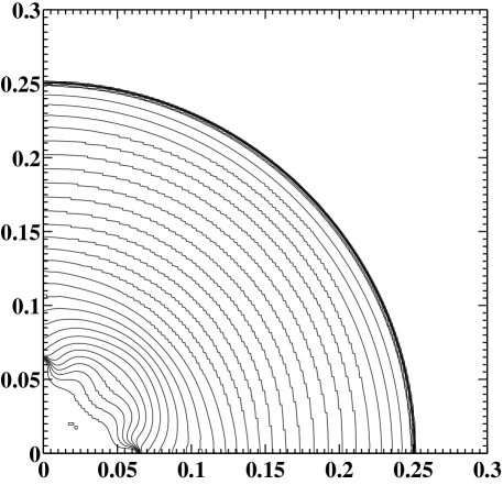
Figure 1: Contour plot of the density logarithm for the run Sedov.2D.b.256.100 at time $t_{tot}=0.9975\cdot 10^{-3}$ (cf. Fig. 2). 30 contour lines correspond to the values of the density logarithm that are equally spaced between its maximum (0.75) and minimum (-3.11) values.

In this type of tests, designated as “Sedov” in Table 1, the computational domain is initialized with a small uniform region of very high pressure. The size of this region, or charge, is one cell at the finest refinement level. High pressure produces a very strong and fast blast wave that propagates outward and quickly decelerates. Once the radius of the blast wave $r_{b}$ becomes much larger than the size of the charge $r_{0}$ the flow can be considered self-similar of the first kind and the only two parameters that completely determine its properties are the initial density $\rho_{0}$ and the initial charge energy $E_{0}$. Structure of the post-shock flow is characterized by the very steep drop in density and pressure behind the blast wave front (e.g., see Figs. 1 and 2). However, while density drops to essentially vacuum in the central region, pressure asymptotes to a constant and typically fairly high value. With good approximation it can be said that pressure remains nearly constant in the inner 50% of the blast wave radius and this inner region is typically called the “pressure plateau”. Since density asymptotically approaches zero inside pressure plateau, temperature asymptotically tends to infinity toward the blast wave origin. Fig. 1 shows the contour plot of the density logarithm in the computational domain for the run Sedov.2D.b.256.100 at the end of the simulation, while Fig. 2 shows the density distribution along the diagonal cut of the computational domain for all runs in 2D and 3D discussed in this work. The full analytic solution for the structure of the flow can be found in [27, 28] and we refer to those works for further details.

As it was discussed in § 2.1, problems involving stationary ambient medium which is dynamically important, including propagation of global shocks, are not optimal applications of the method presented here. However, the extremely demanding conditions presented by this problem for the numerical codes as well as the availability of the analytic solution make this an excellent test problem, which we use to verify the accuracy of our method as well as its convergence properties in the case of flows with discontinuities. The ability of the scheme to converge to the correct analytic solution in this case is crucial to demonstrate the fact that the non-conservative nature of the method does not introduce a systematic error to the solution and the Rankine-Hugoniot conditions are valid in the transformed reference frame $\mathbf{\tilde{X}}$. As was discussed in § 2.2, such verification of validity of shock jump conditions would be even more critical in the cases of non-trivial choices of scaling parameters $\alpha$ and $\beta$ when rigorous analytical proofs of such validity are not available.

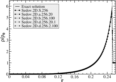
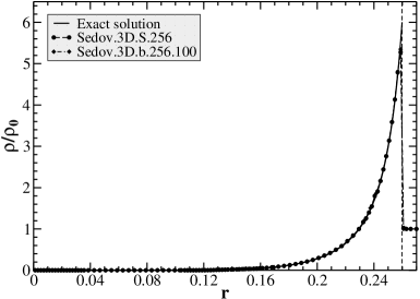
Figure 2: Left: Comparison of runs Sedov.2D at time $t_{tot}=0.9975\cdot 10^{-3}$. Right: Comparison of runs Sedov.3D at time $t_{tot}=0.355\cdot 10^{-3}$. In both panels shown is density along the diagonal cut of the computational domain in the units of ambient density $\rho_{0}$. Vertical dashed line indicates the shock front position based on the exact solution.

This class of tests was carried out with all types of computational reference frames discussed above, except for type c (constant acceleration contracting frame). All tests were compared against the full analytic solution [27] as well as against the results of a corresponding reference simulation performed in the inertial frame. We also carried out this test in three dimensions in the inertial and constant acceleration (type b) frames in order to verify the accuracy of the method in 3D. All 2D and 3D runs, including the ones in the inertial frame, had the same total physical simulation run time $t_{tot}$ (see Table 2). Moreover, it was ensured that in all moving frame runs the domain extent in physical space at the end of the simulation coincided with that of the simulation in the inertial frame. To achieve that in the case of oscillating frame runs the number of oscillation periods was always integer and, thus, the domain extent in physical space was the same at the beginning and the end of the run. This guaranteed that the effective resolution of each run, i.e., cell size in physical space at the finest refinement level, was the same at time $t=t_{tot}$, when cross-comparison of the runs was performed.

Initial conditions in all runs (both 2D and 3D) are as follows. Ambient density is $\rho_{0}=1.0$ and ambient pressure is $P_{0}=10^{-4}$. It should be noted that in order to reproduce the true Sedov blast wave the ambient pressure would have to be set at essentially zero value. While this is possible in the case of a stationary reference frame, in which ambient material velocity is zero, in a moving reference frame that is impossible. The reason for that is the large velocity $\mathbf{\tilde{u}}=-\dot{a}\mathbf{\tilde{r}}$ of the ambient material in the computational frame which is necessary to support the shock. The fact that 100% of the total energy in the ambient material is kinetic energy results in breakdown of the solution in the hydrodynamic solver in cells containing ambient material. On the other hand, the maximum difference (max-norm) between the lowest resolution runs performed in a stationary frame with $P_{0}=10^{-4}$ and $P_{0}=10^{-16}$ is $1.5\cdot 10^{-6}$. This is almost 4 orders of magnitude less than the 1-norm error between the numerical and exact solution (cf. Fig. 7). Hence, we conclude that at the resolutions considered the solutions obtained with $P_{0}=10^{-4}$ are virtually identical to the solutions that would be obtained with $P_{0}=0$. The charge is a cell at the finest refinement level located in the corner of the domain with coordinates $x_{i}=0$. Charge density is $\rho_{0}$ and charge energy is $E_{0}=1000.0$. Initially fluid is at rest in the inertial frame.

All runs were performed in a quadrant in 2D and an octant in 3D. Due to this boundary conditions on the lower $x$, $y$ (and $z$) boundaries were reflective. Boundary conditions on the upper $x$, $y$ (and $z$) boundaries where of the type appropriate for the problems with dynamically important ambient material, as discussed in § 3.

2. Converging shock (Guderley blast wave)

We use the problem of a converging shock, i.e., the so-called Guderley blast wave, as an example of a collapsing environment. In this problem a strong spherical or cylindrical shock is initiated by some mechanism, e.g., a piston or simply a pressure jump in the initial conditions. The shock propagates toward the center of symmetry of the system increasing its strength, i.e., undergoing cumulation, until the moment of collapse. Thus, this problem presents the same complication for the method discussed here as the strong point explosion since the collapsing shock propagates in the medium stationary in the inertial frame. The solution of this problem was first obtained by [29, 30] and we refer to [28] for the detailed discussion (see also references therein). The converging shock is an example of a self-similar problem of the second type. In such problems the value of the similarity exponent $\kappa$ must be found based on the limiting self-similar solution that exists close to the instant of collapse. There is no general analytic form of such limiting solution, consequently it must be determined numerically. In particular, as the shock wave radius decreases, the solution in the region, the radius of which is of the order of the shock radius and is proportional to it, will be approaching the limiting solution thereby giving an approximation of the latter. The only dependence of that limiting solution on the initial conditions will be described by the parameter $A$, which characterizes the intensity of the initial push. The second unique property of a self-similar problem of the second type is the existence of a critical characteristic in the $r,t$ plane, which is of the same family as the shock wave characteristic and which converges with the latter at the moment of collapse. That characteristic defines the region of influence, i.e., the shock wave cannot be affected in any way by the flow outside the region bounded by the critical characteristic and, thus, it does not depend on the outer boundary conditions. Therefore, in solving the problem of the converging shock wave, it is very important to obtain the structure of the flow in the vicinity of the shock front as accurately as possible and as closely to the instant of collapse as possible as that structure is then used to represent the sought limiting solution based on which all of the characteristics of the flow are obtained. Extremely demanding conditions presented by this test for a numerical code, in particular the sharp rise in pressure and temperature and, consequently, the shock strength near the moment of collapse, as well as the availability of a single parameter that is highly sensitive to the quality of the solution, namely the similarity exponent $\kappa$, make this an excellent test for assessment of the performance of this method in the case of contracting reference frames.

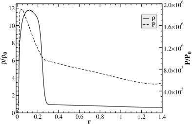
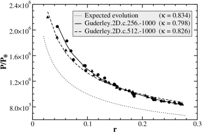
Figure 3: Left: Structure of the converging shock wave right before the shock front collapse at the center of symmetry. Shown is density and pressure, normalized to their pre-shock values $\rho_{0}$ and $P_{0}$, at time $t=0.89\cdot 10^{-3}$. Profiles are taken along the diagonal cut of the computational domain of the run Guderley.2D.S.256. Right: Position and values of pressure maxima for the final stages of collapse of the converging shock. Circles represent pressure maxima at each moment in time for the run Guderley.2D.c.256.-1000, while the triangles show the same for the run Guderley.2D.c.512.-1000. The solid and dashed lines show the corresponding fits for those two runs. The dotted line shows the expected evolution.

All performed simulations of this type of test were carried out in a constant acceleration contracting frame, i.e., type c as discussed in § 4.1. As with other tests, we also performed a reference run in the inertial frame (see Fig. 3). The total duration in physical time of all simulations as well as their initial domain extent in physical space is the same (see Table 1). At the end of the moving frame runs their domain extent in physical space is exactly half that of the reference run, therefore, the final resolution of the run Guderley.2D.c.256.-1000 is twice the resolution of the reference run Guderley.2D.S.256.

Initial distribution of all physical quantities, including fluid velocities, is identical in all runs. Initial density is uniform $\rho_{0}=1.0$. Pressure distribution contains a jump along the interface with the radius $r_{P}=0.8$. Pressure inside the interface is $P_{0}=1.0$, while outside is $P_{out}=10^{6}$. Here, as in the case of the Sedov blast wave, the pre-shock pressure should ideally be set to zero. However, for the same reason as the one discussed before that is impossible in the case of a contracting reference frame. Moreover, in this case we also find that the significant decrease in pre-shock pressure has a negligible effect on the solution. All runs were performed in a quadrant in 2D. Consequently, boundary conditions on the lower $x$ and $y$ boundaries were reflective. As it was said above, the choice of boundary conditions on the upper $x$ and $y$ boundaries does not affect the structure of the flow in the shock vicinity. Thus, we use zero-order extrapolation boundary conditions on the upper $x$ and $y$ boundaries, as it was discussed in § 3.

Left panel of Fig. 3 shows the structure of the flow right before the collapse of the shock front at the center of symmetry. The region, representing the limiting self-similar solution, extends to $r\approx 0.1$. The flow outside that region is completely determined by the initial and boundary conditions. As the shock approaches the point of collapse the pressure and temperature behind the front tend to infinity, while density behind the front stays constant and equal to $[(\gamma+1)/(\gamma-1)]\rho_{0}$. Further behind the front density rises monotonically with radius and eventually it asymptotes to a limiting value $\rho_{lim}$, which is achieved at the moment of collapse. For $\gamma=\,{}^{7}\!/_{5}$ the limiting density is $\rho_{lim}=21.6\rho_{0}$.

The similarity exponent describes the shape of the distribution of basic quantities in the self-similar region immediately behind the shock front. For example, the pressure behind the front is

$$P\sim R^{2(\kappa-1)/\kappa},$$ (57)

where $R$ is the current shock position. Monotonicity of pressure behind the front depends on the value of the polytropic index $\gamma$. For $\gamma=\,{}^{7}\!/_{5}$, used in our simulations, the pressure rises behind the front until it reaches the maximum, after which it monotonically decreases. Thus, in practice in a numerical solution it is much easier to identify the pressure maximum, rather than the value of pressure immediately behind the shock front. Moreover, as can be seen in Fig. 3, such pressure maximum trails the shock front rather closely. Right panel of Fig. 3 shows positions and values of pressure maxima for a sample of times in the runs Guderley.2D.c.256.-1000 and Guderley.2D.c.512.-1000. The moments in time were chosen fairly close to the point of collapse when it is possible to assume that the solution has a large degree of self-similarity. Subsequently, a fit was produced for each run according to eq. (57), based on which the similarity parameter $\kappa$ was determined. The obtained values of $\kappa$ for both runs are shown in the legend. The dotted line shows the expected evolution of maximum pressure, and in the legend the exact theoretical value of $\kappa$ is given.

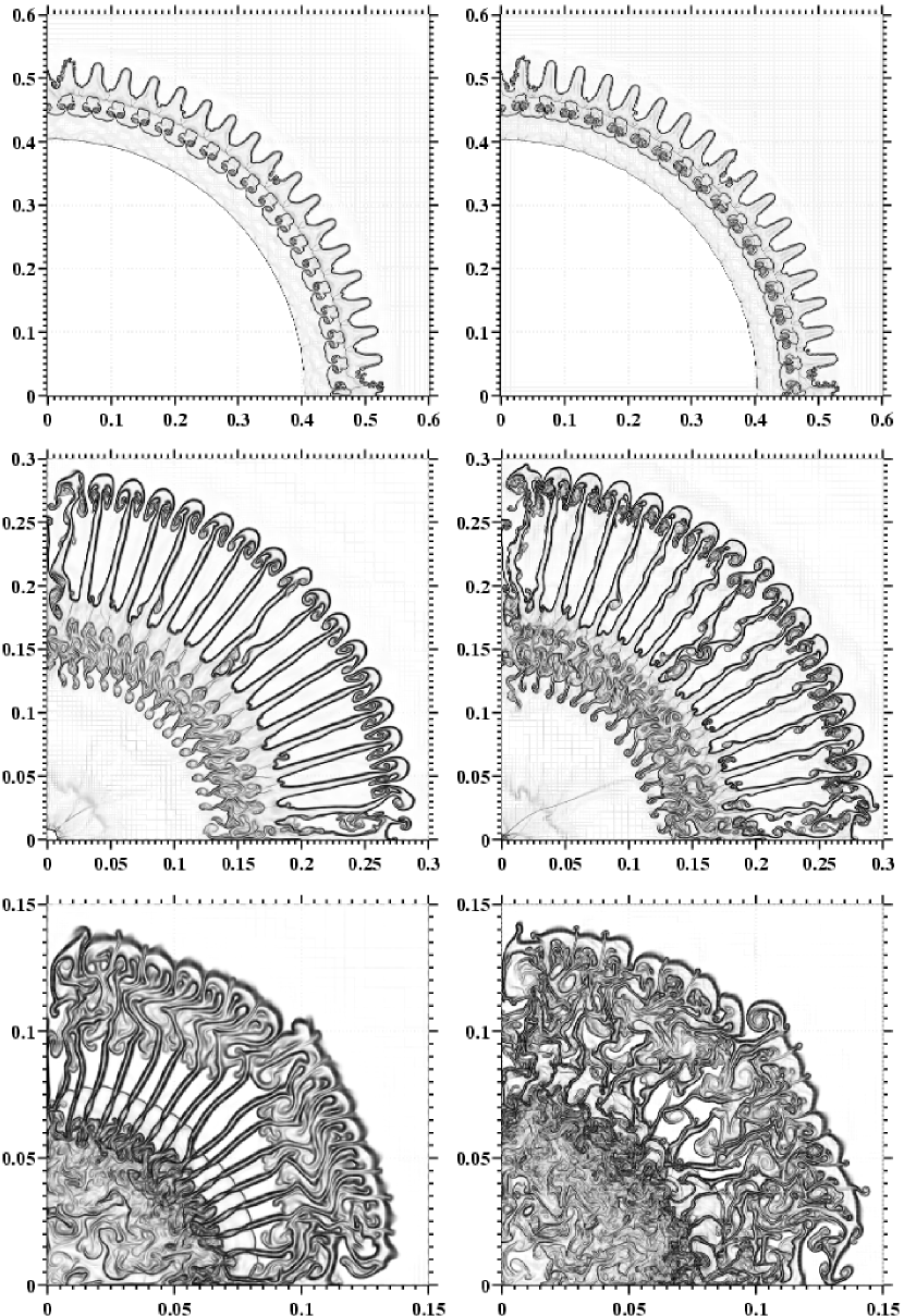
Figure 4: Evolution of the converging shock wave interacting with a density interface with imprinted perturbations. Shown are the Schlieren images of the computational domain of the simulations GuderleyShell.2D.S.4096 (left panels) and GuderleyShell.2D.c.4096.-1250 (right panels) for three moments in time, namely from top to bottom: $t=0.358\cdot 10^{-3}$, $t=0.576\cdot 10^{-3}$, and $t=0.713\cdot 10^{-3}$.

We also conducted a more complicated variation of this test, designated as “GuderleyShell” in Table 1. In that test a converging shock, identical to the one discussed above, interacts with the density interface with imprinted perturbations. This problem is somewhat analogous to the collapse of a fuel pellet in the inertial confinement fusion applications, in which the perturbations are the result of surface nonuniformities of the pellet itself as well as of the nonuniformity of the pellet surface illumination with laser beams. The setup of this test is identical to the one described above, except that besides the pressure jump at $r_{P}=0.8$ there is also a density jump at $r_{\rho}=0.7$ with density inside that interface $\rho_{in}=0.05$. The interface itself is imprinted with a sinusoidal perturbation with amplitude $A=0.015\approx 2\%\,r_{\rho}$ and 18 perturbation periods in a quadrant. We performed a reference run in the inertial frame and a run in the constant acceleration contracting frame. Computational domain setup and domain resolution were identical in both runs at time $t=0$.

The key feature of this problem is the rapid inward growth of perturbations driven by the Rayleigh-Taylor instability due to the presence of dense pressurized shocked material above the interface. Fig. 4 [31] shows the initial stage of the perturbation growth right after the shock impact of the density interface, the intermediate stage, when the perturbation spikes are fully evolved, and the final stage right after the moment of shock front collapse. We use this test to illustrate the difference in the final state of the system due to the two-fold increase in resolution, which is provided by the reference frame contraction in otherwise identical simulations. Such resolution increase is primarily manifested in the flow being much more unstable in the accelerating frame run. Moreover, higher resolution of the central region allowed to achieve higher central peak pressure at the moment of the shock front collapse and, as a result, a faster rebound blast wave propagating outward through the material continuing to collapse. It should be noted that, as it was discussed in § 2.1, in this type of problems involving propagation of a global shock the increase of the physical time step cannot be expected since while the shock velocity is minimal in the contracting reference frame, pre-shock material has large velocity in the computational frame. Nevertheless, in the case of the moving frame with only minimal additional computational effort, primarily due to the $\approx 10\%$ increase in the number of time steps, it was possible to achieve the result that would require twice higher resolution.

3. Expansion of a gas sphere into vacuum

This problem, which is an example of the optimal application of the method presented here, was used to demonstrate efficiency and long term performance of the method in systems that exhibit large degree of expansion. We also use these tests to verify the conservativity properties of the method in a setting fairly representative of its typical realistic application. We consider both an initially stationary (designated as test category “Sphere” in Table 1) and an initially rotating sphere (test category “SphereRot” in Table 1). The latter case allows us to demonstrate the performance of the method with an expanding and rotating reference frame. In all those tests the initial setup of the problem is a sphere of radius $r_{s}=0.3$ with constant initial density $\rho_{s}=10^{3}$ and constant initial pressure $P_{s}=10^{5}$. Ideally ambient conditions for this problem should be vacuous. However, since that is unfeasible in a Eulerian code, ambient conditions were set to have the minimal possible dynamical effect on the expansion of a sphere. In particular, in the reference runs performed in the inertial frame ambient density was $\rho_{0}=10^{-2}$ and ambient pressure was $P_{0}=10^{-2}$ in the non-rotating case and $\rho_{0}=10^{-3}$ and $P_{0}=10^{-3}$ in the rotating case. In the moving frame runs ambient material was set to be stationary in the computational frame and, therefore, it was expanding along with the sphere material. Consequently, it was possible to use higher values for the ambient density and pressure without causing dynamical effects on the expansion of the sphere, namely $\rho_{0}=1.0$ and $P_{0}=1.0$ in the non-rotating case and $\rho_{0}=0.1$ and $P_{0}=0.1$ in the rotating case.

Fig. 5 shows the solution structure for the non-rotating and rotating sphere cases at four different times. Both density and velocity are shown as functions of the similarity variable $r/t$ thereby illustrating gradual development of the self-similar structure by the flow. Fig. 6 shows the temporal evolution in the system of the total kinetic energy measured in the inertial frame for two cases.

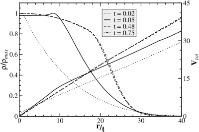
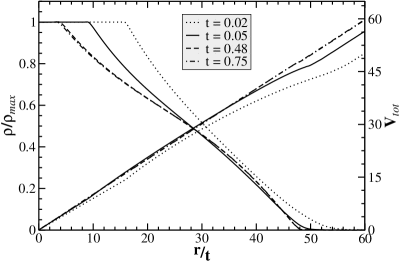
Figure 5: Left: Run Sphere.2D.a.2048.50. Right: Run SphereRot.2D.$\textrm{e}_{2}$.2048.80. Both panels show normalized density (set of decreasing curves) and total velocity (set of increasing curves). Density is normalized to its maximum value at each time. All distributions are given along the diagonal cut of the domain.

In the non-rotating case expansion starts with the outer layer which expands with the maximum escape velocity $u_{max}=[2/(\gamma-1)]c_{s}$, where $c_{s}$ is the initial sound speed in the sphere. For the conditions given above $u_{max}=38.7$. The rarefaction wave propagates toward the sphere center. The time when it reaches the center marks the end of the acceleration phase. At that point all of the sphere material has been disturbed and the linear velocity profile sets in. The dotted lines in Fig. 5 show the density and velocity profiles at that time, i.e., at $t=0.02$. Note that, as can be seen in Fig. 6, at the end of the acceleration phase in the non-rotating case kinetic energy constitutes about 56% of the total energy. After that the rarefaction wave bounces off at the center and the reflected rarefaction starts to propagate outward. This phase is shown with the solid lines in Fig. 5 for $t=0.05$. Initially the flow in the system is not self-similar since there is a characteristic dimension in the problem, namely the initial sphere radius $r_{s}$. However, as the expansion proceeds and the flow extent becomes much larger than $r_{s}$, it eventually “forgets” about the initial conditions and the flow asymptotically approaches the self-similar regime. This can be seen in Fig. 5 as the density and velocity distributions at $t=0.48$ and $t=0.75$ are almost identical.

In the rotating case the initial angular velocity of the sphere is $\omega_{s}=100.0$ (see Table 1). This value was chosen to ensure that initially kinetic and thermal energies of the sphere material are comparable, with the initial kinetic energy due to rotation constituting about 60% of the total energy (see Fig. 6). Evolution of the rotating sphere critically depends on the magnitude of that initial kinetic energy. Our choice of the angular velocity ensured, on one hand, an important role of the acceleration phase during which the rarefaction wave traveled into the sphere interior and the kinetic energy rose from 60% to about 95% of the total energy (see Fig. 6). The dotted lines in the right panel of Fig. 5 show the flow structure at the end of that phase, i.e., at $t=0.02$. On the other hand, the rarefaction wave never reached the center and, thus, the reflected rarefaction was never produced as can be seen in the absence of the characteristic bump in the solid line showing density at $t=0.05$ (cf. the solid line for the same time in Fig. 5). Note also that in the rotating sphere the expansion velocity is higher than in the non-rotating one due to the centrifugal force acting on the rotating fluid. Consequently, the flow tends to “forget” the initial conditions much sooner and, therefore, to approach the self-similar regime much more rapidly.

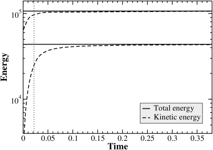
Figure 6: Temporal evolution of the kinetic energy in the case of expansion of a non-rotating sphere (lower pair of curves, run Sphere.2D.a.2048.50) and a rotating sphere (upper pair of curves, run SphereRot.2D.$\textrm{e}_{2}$.2048.80) into vacuum. Shown only the first half of the total physical simulation run time. Vertical dashed line corresponds to the total run time of the runs Sphere.2D.S and SphereRot.2D.S.

In performing those tests we used only the reference frames that are most suited for this type of problems and can provide the optimal performance in the absence of fluid motions feedback. For both the non-rotating and rotating cases we also carried out a series of reference runs in the inertial laboratory frame. In the non-rotating case the most natural choice for the reference frame was the constant velocity expanding frame (runs Sphere.2D.a in Table 1). During the acceleration phase, however, the linear velocity profile gradually extends inward along with the rarefaction wave propagating inward. In the computational frame that results in the sphere material initially possessing a large velocity gradient $\mathbf{\tilde{u}}=-\dot{a}\mathbf{\tilde{r}}$ (see eq. (7)) which is slowly being eliminated as the fluid accelerates until all of the sphere material is comoving with the reference frame. The initial presence of such velocity gradient can cause the degradation of the solution. In a realistic application a feedback mechanism would cause the reference frame to accelerate gradually until the linear velocity profile is established thereby eliminating such a problem. In order to assess the improvement of the solution due to such more accurate tracking of fluid motions, we carried out a set of simulations utilizing the delayed stretch reference frame, i.e., type $\textrm{a}_{d}$ as discussed in § 4.1, designed to imitate the action of such a realistic feedback mechanism (runs Sphere.2D.$\textrm{a}_{d}$ in Table 1). Those simulations were initialized by transforming the computational domain of the reference inertial frame runs at time $t_{s}=0.021$ to the constant velocity expanding frame.

In the case of a rotating sphere angular velocity of the fluid resulted in all of it having a radial expansion velocity from $t=0$. Therefore, with a good approximation throughout the acceleration phase the interior of the sphere could be characterized by the linear velocity profile. That justified the use of an expanding frame for the whole duration of the runs and eliminated the need for the use of the delayed stretch. At the same time in the process of expansion the fluid quickly loses its angular velocity due to the conservation of angular momentum. In order to account for that we used the constant velocity expanding frame with expansion-correlated angular velocity, i.e., type $\textrm{e}_{2}$ as discussed in § 4.1 (runs Sphere.2D.$\textrm{e}_{2}$ in Table 1). In both the non-rotating and rotating cases the grid velocity $v_{g}$ was chosen to be slightly lower than the expansion velocity of the sphere. For example, in the runs Sphere.2D.a velocity $v_{g}$ of the grid right boundaries with coordinates $\tilde{r}_{b}=0.6$ (see Table 2) was 50.0 (see Table 1). Thus, initially at the sphere boundary $\tilde{r}_{s}=0.3$ grid velocity was $v_{g,s}=(v_{g}/\tilde{r}_{b})\tilde{r}_{s}=25.0$ which is lower than the maximum expansion velocity into vacuum $u_{max}=38.7$. Therefore, sphere material in all moving frame simulations initially expanded somewhat until the outer layer of the sphere reached the point in the domain with matching grid velocity.

The non-rotating sphere runs were performed in a quadrant with the sphere center located in the lower left corner of the domain. In the rotating case, the domain contained the full sphere in order to accommodate its rotation with the sphere center and the fixed point of reference frame expansion located in the center of the computational domain. We carried out each type of runs with a range of resolutions. The total time $t_{tot}$, given in Table 2, of the reference runs performed in the inertial frame was chosen to cover the duration of the acceleration phase of the expansion. Correspondingly, the domain size in those runs was set to accommodate the expansion of the sphere during that time. In the moving frame runs, with the exception of the delayed stretch runs Sphere.2D.$\textrm{a}_{d}$, the domain size was chosen to be half the size of the domain in the reference runs, since the sphere does not expand significantly in the computational frame. Therefore, at $t=0$ the computational domain in the moving frame coincides with the inner half of the domain of the corresponding reference runs. Thus, initially cell size in physical and computational space is identical for all runs at a given resolution level.

Finally, since ambient material in all simulations was set to be stationary in the current reference frame, boundary conditions in the case of a non-rotating sphere were of the reflective type on all domain boundaries as discussed in § 3. This allowed us to use those runs for the study of the conservativity properties of the method in § 4.4 below. In the simulations of a rotating sphere boundary conditions were of the zero-order extrapolation type on all boundaries.

4. Isentropic expansion with an embedded density structure

The fourth type of tests we conducted is the isentropic expansion of a uniform pressure field with an embedded density structure (test category “Clump” in Table 1). The initial setup of the problem is the computational domain with constant initial pressure $P_{0}=1.0$. The embedded density structure is a circular clump with uniform density $\rho_{c}=10^{3}$ while ambient density is $\rho_{0}=1.0$. Clump radius is $r_{c}=0.15$ and its center has coordinates $\tilde{x}_{i}=0.3$. All fluid has constant expansion velocity $u_{i}=\dot{a}\tilde{x}_{i}$, where $\dot{a}$ is such that both components of the clump center velocity are equal to $50.0$. The computations are performed in the reference frame co-expanding with the fluid with the center of expansion located in the lower left corner of the domain. Consequently, all boundaries have perfectly reflecting boundary conditions.

In the course of its evolution the domain expands by more than two orders of magnitude while pressure drops to $10^{-7}$ and clump density drops to $0.063$. In this problem the exact structure of the flow at time $t_{tot}$ can be determined analytically, moreover the clump boundary must remain as a sharp discontinuity. Consequently, we use this test to verify the second order convergence of the numerical solution to the exact one.

4.3 Test results: method accuracy

There are two principal sources of errors in the strategy employed by us for solving the system (11) - (13), i.e., operator splitting. They are, on one hand, the numerical errors introduced individually by the hydrodynamic and source term solvers and, on the other hand, the errors due to the imbalance that can arise during a time step between the two solvers.

In order to illustrate the origin of the first source of errors consider the action of the two operators in the course of one time step in the case of direct operator splitting as described by the eq. (25). It is convenient to rewrite that equation as follows

$$\begin{array}[]{rcl}\tilde{q}^{n+1}=\mathcal{S}^{(\Delta t)}\mathcal{H}^{(\Delta t)}\tilde{q}^{n}&\,=&\mathcal{S}^{(\Delta t)}\left(\tilde{q}^{*,n+1}_{H}+\delta\tilde{q}^{n+1}_{H}\right)=\\ &&\tilde{q}^{*,n+1}+\delta\tilde{q}^{n+1}_{S}+\delta\tilde{q}^{n+1}_{HS}+\delta^{2}\tilde{q}^{n+1}_{HS}.\end{array}$$

The solution is first advanced over the full step $\Delta t$ with a hydrodynamic solver. The resulting solution consists of the exact solution $\tilde{q}^{*,n+1}_{H}$ of the homogeneous part of the original equations and the numerical error $\delta\tilde{q}^{n+1}_{H}$ introduced by the solver. That error does not violate the conservativity of the solution, provided that the hydrodynamic scheme is conservative. After that source terms are applied adjusting the obtained solution to account for the effects of grid expansion/contraction and to apply forces due to the grid acceleration and/or rotation. Thus the final solution at the end of the time step consists of the exact solution $\tilde{q}^{*,n+1}$ of the full equations and the error $\delta\tilde{q}^{n+1}_{S}$ produced by the source term solver acting on the exact part $\tilde{q}^{*,n+1}_{H}$ of the homogeneous solution, as well as the errors $\delta\tilde{q}^{n+1}_{HS}$ and $\delta^{2}\tilde{q}^{n+1}_{HS}$ due to the source term solver action on the error $\delta\tilde{q}^{n+1}_{H}$. The error $\delta\tilde{q}^{n+1}_{HS}$ is the “exact” part of the result of the application of the source term operator $\mathcal{S}$ to the hydrodynamic error $\delta\tilde{q}^{n+1}_{H}$, therefore, it does not violate the conservativity of the final solution. That is not the case for the other two errors since the source term solver simply adds or subtracts a certain amount of state vector components in each cell. A small numerical error in that amount, i.e., the sum of errors $\delta\tilde{q}^{n+1}_{S}$ and $\delta^{2}\tilde{q}^{n+1}_{HS}$, results in violation of conservativity. As was discussed in § 3, we use the second-order accurate conservative explicit hydrodynamic schemes and the fourth-order accurate implicit source term solver. Consequently, the error $\delta\tilde{q}^{n+1}_{HS}$ has the largest effect on the accuracy of the solution. It drops quadratically with the decrease in spatial and temporal step. The error $\delta\tilde{q}^{n+1}_{S}$ is significantly smaller due to the much higher accuracy of the source term solver, moreover it decreases as the $4^{th}$ power of the spatial and temporal step. Finally, the error $\delta^{2}\tilde{q}^{n+1}_{HS}$ has the smallest magnitude. It does not have a unique dependence on the spatial and temporal steps since the “exact” solution $\delta\tilde{q}^{n+1}_{HS}$ itself changes with resolution.

Aside from employing more accurate hydrodynamic schemes or using the brute force approach of higher resolution, the most efficient way to minimize all of the above errors is by closely correlating the motion of the non-inertial frame with the fluid motion and, thereby, by minimizing the velocity field in the computational domain. However, that will have the largest effect on the error $\delta\tilde{q}^{n+1}_{HS}$ since it typically dominates other errors. In the limit of the reference frame perfectly following the fluid motion so that the material is stationary in the computational domain, the hydrodynamic solver does not alter the solution during a time step, as no waves are produced at cell interfaces, and, therefore, it does not produce the error $\delta\tilde{q}^{n+1}_{H}$. Consequently, the error $\delta^{2}\tilde{q}^{n+1}_{HS}$ is also absent. However, the error $\delta\tilde{q}^{n+1}_{S}$ would still be present. In § 4.4 and § 4.5 we illustrate the effect this can have on the conservativity and convergence properties of the solution. The first and last errors in eq. (4.3) can be further minimized by increasing the accuracy of the source term solver. One of the major advantages of the Kaps-Rentrop method, used by us, is the fact that this scheme is embedded, i.e., it provides means to control the solver accuracy or, equivalently, the magnitude of the relative error of the solution. In all simulations discussed in this work we use the target value of the relative error of $10^{-4}$. We found it to be the most optimal compromise between speed and accuracy of the solver. However, even infinite accuracy of the latter would not completely eliminate the error $\delta\tilde{q}_{HS}^{n+1}$ since there is always a seed present $\delta\tilde{q}^{n+1}_{H}$.

The second source of numerical errors is the imbalance between the action of the hydrodynamic and source term operators during a time step. It can be seen from the eqs. (11) - (13) as well as the expressions for $d\ln a/d\tau^{\prime}$, $d^{2}\ln a/d\tau^{\prime 2}$, and $d\ln\Omega/d\tau^{\prime}$ given in § 4.1 that source terms usually depend explicitly on time, i.e., grid velocity $\dot{a}(t)$ can vary substantially in the course of one time step. We found that two techniques can be very efficient in maintaining balance between the two operators. Firstly, in § 3 it was discussed that in our source term solver we use time step subcycling. Consequently, in the course of such subcycling source terms and their Jacobian $A_{ij}$ at each substep must be evaluated using the value of $t$ that corresponds to the beginning of the global time step. This also applies to both substeps in the case of Strang splitting. The second technique is limiting the time step, at which the simulation is advanced, in correspondence with the rate of change of the source terms, namely

$$d\tau=\displaystyle\alpha\min\left\{d\tau_{H},\left|\tilde{q}_{p}\left(\frac{d\tilde{q}_{p}}{d\tau^{\prime}}\right)^{-1}\right|\right\},$$ (58)

where $d\tau_{H}$ is the next time step determined based on the CFL condition (27) and the factor $\alpha$ is typically $0.05-0.1$. Subscript $p$ indicates the state vector components that represent density and energy. We do not use momenta in the determination of the time step as they can have zero values. Values for $d\tilde{q}_{p}/d\tau^{\prime}$ are simply found based on the right-hand side of the original equations. The above prescription ensures that source terms do not vary significantly within one time step thereby allowing the hydrodynamics to adjust appropriately to the changes in the velocity of the reference frame.

AMR can serve as an additional source of errors when an insufficiently accurate interpolation technique is used in the process of refining a certain region. Consider the fluid of uniform density and pressure stationary in the inertial reference frame. Assume that the computational domain resolution is increased from $dx$ to $dx/2$. While density and pressure are uniform and constant throughout the domain, the velocity gradient $\mathbf{\tilde{u}}=-\dot{a}\mathbf{\tilde{r}}$ would have to be interpolated appropriately to the new resolution. Assume that constant interpolation is used. Then in two adjacent fine cells, which replaced one coarse cell, velocity will be the same instead of representing the velocity gradient. This will lead to the creation of artifact features in the computational domain. The use of higher order interpolation techniques, e.g., centered linear interpolation, significantly removes such artifacts although at a certain level they are always present.

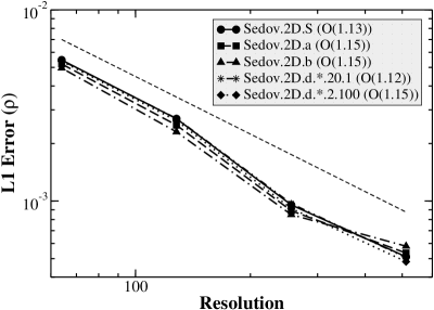
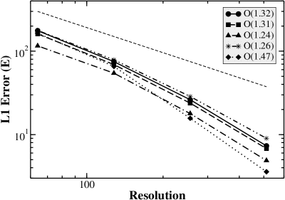
Figure 7: Convergence of the numerical solution to the exact one in simulations of the Sedov blast wave in various reference frames. Left: $L1$ error in density. Right: $L1$ error in total energy in the laboratory reference frame. The order of convergence is shown in brackets in the legend in both panels. The dashed lines correspond to first-order convergence.

Figs. 1, 2 and 7 illustrate the overall accuracy of the method presented here for the case of the strong point explosion test, discussed in § 4.2. Note in Fig. 1 that the overall sphericity and azimuthal uniformity of the solution is preserved and no artifacts along the axes were introduced neither by the hydrodynamic scheme, nor due to the fact that the simulation was performed in the expanding non-inertial reference frame. The only exception is the central vacuous region in which internal energy becomes extremely high. However due to the presence of singularity at the center in the exact solution the numerical solution in that region obtained with practically any Eulerian code would significantly differ from the analytic one. Fig. 7 shows the convergence of the $L1$ error in density and total energy between the numerical and exact solutions in simulations of the Sedov blast wave. It can be seen in Fig. 7 (see also Fig. 2) that even for a fairly low resolution of 64 cells the solution accuracy in the moving frame runs is rather high. More importantly, it can be seen in Fig. 7 that even in this test, which is not an optimal application of this method, the solution accuracy practically for all types of moving frames is equal to or greater than the accuracy of the solution in the laboratory frame. The only exception are the higher resolution runs performed in the high amplitude low frequency oscillating reference frame in which the solution has a slightly higher error in energy. That shows that the computation in a moving frame does not introduce a systematic error and the numerical solution properly converges to the exact one.

One important point, that follows from Figs. 2 and 7, concerns the behavior of the runs performed in the oscillating reference frames. It is unlikely that in realistic applications the frame motion would be smooth as it is in the runs with the constant velocity or constant acceleration frames. Consequently, it is important to assess what level of oscillatory noise is acceptable in the frame motion in order to determine how one should set up the filtering in the fluid motion feedback mechanism. The run Sedov.2D.d.256.20.1 was designed to simulate the low frequency high amplitude oscillations of the frame while the run Sedov.2D.d.256.2.100 was intended to simulate the high frequency low amplitude noise. In both runs, in particular in the latter one, source terms have a very high degree of temporal variability. Therefore, it is essential to use time step limiting as described by eq. (58), without which the solution quality dramatically degrades. With the proper use of such step limiting it is possible to have very high frequency oscillations of the reference frame and still have the solution to virtually coincide with the reference run performed in the inertial frame. It is very important to note, though, that the time step determined according to eq. (58) can be much lower than the maximum time step allowed for this method, based on eq. (27), and that can adversely impact the overall performance of the method. In fact, the run Sedov.2D.d.256.2.100 took 110877 steps vs. 6365 steps for the run Sedov.2D.d.256.20.1, 6512 steps for the run Sedov.2D.a.256.20 and 7756 steps for the run Sedov.2D.b.256.100. Therefore, while the method discussed in this work allows one to accommodate high frequency oscillations of the frame without any significant loss of accuracy, it is beneficial for the code performance to filter out such high frequency noise and only to follow smooth global motions of the fluid. Of course, a healthy balance must be found between that and still closely tracking the fluid motions since, as was discussed above, the loss of such close correlation increases the error introduced by the hydrodynamic solver.

Solution accuracy in the case of the contracting reference frame, considered for the problem of the converging shock, is illustrated in the right panel of Fig. 3. It can be seen that for the lower resolution run the error in the similarity exponent $\kappa$, determined based on the numerical solution, is about 4.3%, while for the run with twice higher resolution the error drops by more than a factor of 4 and is slightly less than 1%. Therefore, in such a numerically challenging test, which is not an optimal application of the method presented here, as was discussed before, it is possible to achieve exceptional solution accuracy with contracting reference frames even in the cases of modest resolution.

The above discussion of the method accuracy is also valid when solving the system (11) - (13) with a different choice of scaling parameters $\alpha$ and $\beta$, in particular the one given by (18) and providing conservation of mass. In performing the same strong point explosion tests as the ones discussed above with such choice of $\alpha$ and $\beta$ the accuracy is marginally better due to the fact that the source term solver does not introduce the error in density. In cases in which system evolution is followed over much longer time periods such improvement in accuracy can be more prominent. That effect can be even more pronounced for less accurate source term solvers, in particular the ones with accuracy comparable to that of the hydrodynamic solver. In those cases the choice (18) of $\alpha$ and $\beta$ ensuring conservation of mass (and momentum in constant velocity frames) may significantly improve solution accuracy. Scaling parameter choice can also have an impact on the method performance due to the time step restriction given by eq. (58). Indeed, the absolute magnitude of the source terms and, thus, the rate of change of the state vector may vary depending on the form of the source terms given by different choices of scaling parameters. Finally, solution accuracy can be further increased by the use of Strang splitting. However, in tests discussed here we find this to lead to only marginal solution improvement, moreover in discontinuous flows the convergence rate remains first order in the case of Strang splitting, which, on the other hand, can have significantly larger computational cost.

4.4 Test results: conservativity properties

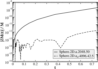
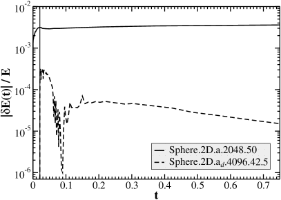
Figure 8: Temporal evolution of the relative error in total mass (left) and total energy (right) conservation for the simulations of expansion of a non-rotating sphere into vacuum. Vertical line indicates the time of start of the reference frame expansion for the run Sphere.2D.$a_{d}$.4096.42.5.

Solving the system (11) - (13) via an operator splitting technique inevitably leads to conservativity errors when the solution is transformed back to the inertial frame. Therefore, it is extremely important to assess the price in conservativity that is being paid by using this method as well as possible ways to control and minimize such errors.

It was discussed in § 4.3 that the main cause of conservativity violation are the errors $\delta\tilde{q}^{n+1}_{S}$ and $\delta^{2}\tilde{q}^{n+1}_{HS}$ (see eq. (4.3)). Consider Fig. 8 which shows temporal evolution of the relative error in total mass and energy conservation in the highest resolution simulations of expansion of a non-rotating sphere into vacuum. The overall behavior is rather similar in both runs. One point should be noted, though, which is not as obvious due to the logarithmic scale. The growth rate of the conservativity errors is increasing in time, except for the error in total energy in the delayed stretch run. That is the manifestation of the fact that the errors $\delta\tilde{q}^{n+1}_{S}$ and $\delta^{2}\tilde{q}^{n+1}_{HS}$ indicated in eq. (4.3) accumulate at each time step and the source term operator, acting on them at the subsequent step, produces an even larger error. Therefore, it is very important to minimize them. Aside from the brute force resolution increase, closely adjusting the moving frame velocity to the fluid velocity is the only method that does not penalize the performance and, instead, can cause a significant speed up due to larger time steps in the computational domain. Indeed, in the case of the delayed stretch run, which did not have during the acceleration phase a significant velocity mismatch characteristic of the run Sphere.2D.a.2048.50, the conservativity error is two-three orders of magnitude lower. In fact, the error in total energy conservation in case of the delayed stretch even shows the decreasing trend. In both runs, as mentioned above, the magnitude of the errors could have been reduced even further by decreasing the target relative error in the implicit source term solver from the value of $10^{-4}$ used in these simulations. By reducing that value down to $10^{-12}-10^{-13}$ we were able to decrease the conservativity errors essentially to the order of machine precision. On the other hand, that also resulted in about an order of magnitude slower performance of the solver due to the much higher number of iterations needed to provide the requested level of accuracy. We also find that the use of Strang splitting can have a much more profound effect on the conservativity of the solution than on its accuracy. In particular, in this case the error in mass and total energy conservation can be additionally decreased by about 2 orders of magnitude for each resolution.

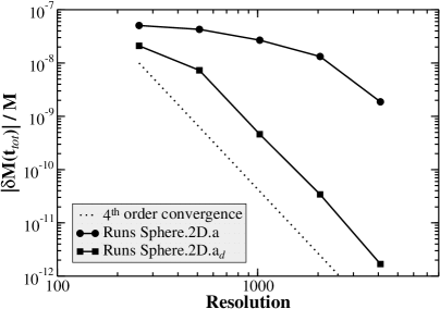
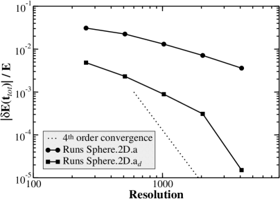
Figure 9: Dependence of the final relative error in total mass (left) and total energy (right) conservation on resolution for the simulations of expansion of a non-rotating sphere into vacuum.

Figure 9 shows that the use of the delayed stretch consistently results in much lower conservation errors at all resolutions. Moreover, the use of the delayed stretch not only significantly reduces the magnitude of the error, but also increases the rate at which it drops with increasing resolution. The dashed line in both figures indicates the rate of the conservation error decrease proportional to the inverse $4^{th}$ power of the resolution. That would correspond to the ideal rate of decrease in the case when the only contribution to the conservation error is due to the term $\delta\tilde{q}^{n+1}_{S}$ in eq. (4.3), which drops as the $4^{th}$ power of the spatial and temporal step. As previously discussed, such situation would correspond to the case when the error $\delta\tilde{q}^{n+1}_{HS}$ due the hydrodynamic solver becomes very small, thus essentially removing the seed for the second contributor to the conservation error, namely the error $\delta^{2}\tilde{q}^{n+1}_{HS}$. Indeed, such behavior is characteristic only of the delayed stretch runs.

Finally, it should be noted that, as was discussed in § 2.2, given the choice (18) of scaling parameters $\alpha$ and $\beta$ it is possible to always conserve mass. Moreover, in the tests considered above momentum would also be conserved since the runs were performed in a constant velocity frame.

4.5 Test results: method convergence

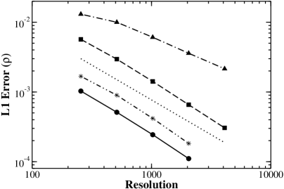
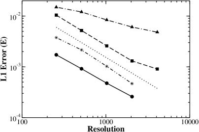
Figure 10: Convergence of the $L1$ error in density (left) and total energy (right) for the simulations of expansion of a non-rotating sphere into vacuum. Dotted lines show the expected rate of convergence. Left: Circles: convergence of runs Sphere.2D.S.256 - 2048 to the run Sphere.2D.S.4096 at $t=0.024$ (order of convergence $O(1.04)$); Squares: convergence of runs Sphere.2D.a.128 - 2048.50 to the run Sphere.2D.S.4096 at $t=0.024$ ($O(1.0)$); Triangles: convergence of runs Sphere.2D.a.128 - 2048.50 to the run Sphere.2D.$\textrm{a}_{d}$.4096.42.5 at $t=0.75$ ($O(0.6)$); Stars: convergence of runs Sphere.2D.$\textrm{a}_{d}$.256 - 2048.42.5 to the run Sphere.2D.$\textrm{a}_{d}$.4096.42.5 at $t=0.75$ ($O(0.98)$). Right: Order of convergence: Circles - $O(0.92)$; Squares - $O(0.99)$; Triangles - $O(0.42)$; Stars - $O(0.92)$.

Another crucial indicator of the quality of a numerical method is its convergence properties. Fig. 7 shows the convergence of the numerical solution to the exact one in simulations of the Sedov blast wave. It can be seen that the convergence rate is first-order as would be expected for the case of a discontinuous flow. Moreover, the convergence rate is fairly insensitive to the type of the moving frame used. Interestingly, the total energy shows the convergence rate that is higher than that of density.

We also consider the convergence of the solutions obtained in the simulations of expansion of a non-rotating and a rotating sphere into vacuum at the early stage of system evolution, i.e., at the end of the acceleration phase, as well as at the later stage when the flow expansion is quite substantial. The results are shown in Figs. 10 - 11, giving the convergence of the $L1$ error in density and total energy. Note, that the resulting $L1$ error was normalized to the maximum value of the given quantity $q_{p,max}$ in the solution profile of the run being considered in order to allow error comparison at early and late stages of system evolution. Since the reference run always has the highest resolution, its diagonal cut was interpolated individually to the points of each run, being studied for convergence.

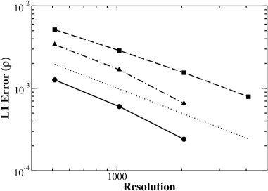
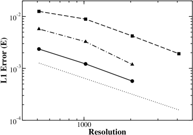
Figure 11: Convergence of the $L1$ error in density (left) and total energy (right) for the simulations of expansion of a rotating sphere into vacuum. Dotted lines show the expected rate of convergence. Left: Circles: convergence of runs SphereRot.2D.S.512 - 2048.80 to the run SphereRot.2D.S.4096 at $t=0.02$ (order of convergence $O(1.13)$); Squares: convergence of runs SphereRot.2D.$\textrm{e}_{2}$.256 - 2048.80 to the run SphereRot.2D.S.4096 at $t=0.02$ ($O(0.87)$); Triangles: convergence of runs SphereRot.2D.$\textrm{e}_{2}$.256 - 1024.80 to the run SphereRot.2D.$\textrm{e}_{2}$.2048.80 at $t=0.75$ ($O(1.1)$). Right: Order of convergence: Circles - $O(0.99)$; Squares - $O(0.76)$; Triangles - $O(0.98)$.

The reference “exact” solution at the end of the acceleration phase was taken based on the highest resolution run performed in the inertial reference frame, i.e., the run Sphere.2D.S.4096 in the non-rotating case and the run SphereRot.2D.S.4096 in the rotating case. The reference “exact” solution in the case of a non-rotating sphere at $t_{tot}=0.75$, i.e., when the sphere has expanded by almost two orders of magnitude, was the highest resolution run performed with the delayed stretch, namely the run Sphere.2D.$\textrm{a}_{d}$.4096.42.5. The reference “exact” solution in the case of a rotating sphere at $t_{tot}=0.75$ was the highest resolution run performed in the expanding and rotating reference frame, i.e., the run SphereRot.2D.$\textrm{e}_{2}$.4096.80. The caption of each figure indicates the order of convergence for each curve. The convergence in all cases is first-order. The only exception is the lower convergence rate at a later stage of the runs performed without the delayed stretch, i.e., the dash-dotted line. The reason for that is the contamination of the solution by a large error due to the significant mismatch between the velocities of the global flow and the reference frame during the acceleration phase, as was discussed in § 4.3 and § 4.4. Fig. 11 shows that similar results are produced in the case of a rotating sphere as well. Ideally, the flow in such system should be smooth. Consequently the use of the second-order scheme should lead to the second-order convergence. In practice, however, there is always a discontinuity present in the problem as the result of the propagation of the sphere material into the ambient medium. In an ideal situation ambient density would have to be set at zero which is impossible in a Eulerian code. Therefore, even though the ambient density can be very small it still produces a discontinuity thereby decreasing the order of convergence of the overall solution.

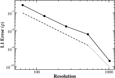
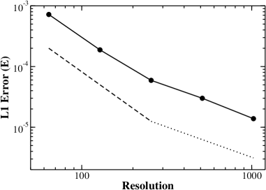
Figure 12: Convergence of the $L1$ error in density (left) and total energy (right) in runs Clump.2D.a.*.100. Dashed line in both panels corresponds to second-order convergence, while the dotted line in the left panel corresponds to fourth-order convergence and in the right panel - to first-order convergence. Overall convergence order in density is $O(2.01)$ and total energy is $O(1.88)$.

Fig. 12 shows the convergence of the $L1$ error in density and total energy in the simulations of isentropic expansion of a uniform pressure field with the embedded density structure. In this case second-order convergence of the numerical solution to the exact one is achieved. Moreover, the density discontinuity remains sharp throughout the duration of the simulations. The convergence rate in total energy for the two highest resolution simulations drops to first order due to the fact that the errors in density and pressure become small enough so that the overall solution in total energy becomes affected by the error arising as a result of the transformation of the solution to the laboratory reference frame.

5 Discussion and Conclusions

We have presented the method for computation of fluid flows characterized by the following two properties: (1) large degree of expansion/contraction on the evolutionary timescale; (2) domination of the flow velocity field by the global component associated with expansion/contraction and/or rotation of the flow. The key of the method is the transformation $\mathbf{\Lambda}$ (eq. (4)) of the computational domain to a non-inertial reference frame that is comoving with the global flow. Consequently, the fluid variable fields, including velocity, are transformed according to the eqs. (7), (10), (14). The formulation based on such general scaling transformation of the fluid variable fields provides a large degree of flexibility in terms of the form of the source terms which can be suited to the needs of a particular problem. Transition to a moving frame allows to accommodate naturally large changes of the flow extent. Moreover, treatment of rapidly rotating flows, e.g., compact stars and stellar cores, is naturally incorporated in this framework. We also showed that the conservative formulation of the equations of fluid dynamics exists only in the case of restricted reference frame transformations, namely only for non-rotating reference frames expanding/contracting with a constant velocity, and only for the polytropic index $\gamma=1+\,{}^{2}\!/_{\nu}$.

The first key advantage of this approach over other methods that can be used for computation of such flows, namely the AMR and traditional moving mesh techniques, is the fact that thermal and local kinetic energies are comparable in magnitude in the moving reference frame, thereby eliminating the high Mach number problem. All moving mesh methods operate in the inertial frame $\mathbf{X}$, moreover practically all of them are designed to evolve the total energy of the flow. To illustrate the consequences such approaches have on the solution we performed the test Sphere.2D.a.256.50 involving expansion of a non-rotating sphere into vacuum with the Zeus-MP code (v. 2.0.2) [13]. The problem setup was identical to the one described in § 4.2 with one exception. In our simulations ambient material is set to be co-expanding with the reference frame in order to minimize its dynamical effects on the expanding material of the sphere. Setting ambient material to co-expand with the computational grid proved to be impossible in our Zeus-MP simulation since the overwhelming dominance of the total energy of the ambient material by its kinetic component causes an immediate breakdown of the solution. Therefore, we set ambient material to be stationary in the laboratory frame. The grid motion was prescribed to be identical to the grid motion in our simulations and outflow boundary conditions were used on outer domain boundaries, while perfectly reflective boundary conditions were used on the boundaries containing the fixed point of expansion. The run was performed with CFL = 0.5 and artificial viscosity parameter was set to 2.0. Result of the simulation is shown in Fig. 13. The solid line shows the density distribution along the diagonal cut of the domain in our Zeus-MP run, while the dashed line shows for reference the result obtained in the simulation using the method presented here. The complete breakdown of the solution can be seen in the figure. As the outer layers start to expand and their velocity increases thereby rapidly increasing the fraction of the kinetic part of total energy the pressure structure of the rarefaction wave starts to degrade dramatically. The accumulating errors in pressure propagate inward with the rarefaction wave very rapidly completely destroying the solution. All of moving mesh techniques that evolve total energy would suffer from the same problem, albeit to a different extent depending on spatial and temporal accuracy of their hydrodynamic scheme. There exist moving mesh algorithms that evolve internal energy. In particular, Zeus-MP is capable of operating in such a mode and in that case it produces results comparable to the ones obtained with the method presented in this work. Such schemes are also non-conservative, however, unlike the method presented here there are no means in them to control the magnitude of the conservativity error besides the brute force method of resolution increase. Moreover the conservativity error would converge with at most the order of the scheme, e.g., second order, while in our method it is possible to achieve fourth-order convergence of the conservativity error, as was shown in § 4.4.

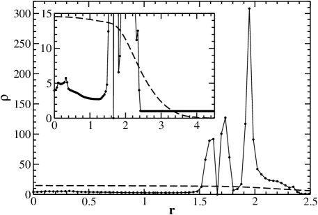
Figure 13: Test Sphere.2D.a.256.50 performed with Zeus-MP (solid line). Shown is the diagonal cut through the domain at $t=0.12$. Dashed line shows the reference solution obtained with the method presented here. Inset shows the zoom-in of the main graph.

It is also important to emphasize that moving mesh algorithms, especially the ones that evolve internal energy, are tightly coupled to a particular implementation of a hydrodynamic scheme which may not be appropriate for all problems when, for example, a higher order scheme might be required. The key practical advantage of the method presented here is the form-invariance of the homogeneous part of fluid equations. Consequently, eqs. (11) - (13) allow for their very easy implementation in a numerical code since all of the effects associated with the moving frame are provided for by source terms. The latter can be solved via operator splitting techniques and there exist very accurate and efficient methods for solving such systems of ordinary differential equations. Unlike the case of the moving mesh formulation (16) which redefines the state vector and the flux functions and thus could require major changes in the hydrodynamic solvers of numerical codes, the formulation discussed here does not affect the hydrodynamic solvers. Thus it allows essentially for the implementation of one general source term integrator that can then be easily combined with any Eulerian hydrodynamic scheme and AMR strategy and, therefore, can utilize the wide potential of existing techniques for solving systems of hyperbolic equations. In particular, we have demonstrated performance of the method in combination with the second-order dimensionally split hydrodynamic scheme used with cell-based AMR (Alla code) and the second-order unsplit scheme using grid-based AMR (AstroBEAR code). Such portability of the method may be especially beneficial in combining this approach with more involved hydrodynamic schemes, in particular implicit and low Mach number solvers for which there may exist no immediate implementation for the solution of the equations similar to eq. (16) and which may provide further improvements in efficiency in problems in which the local velocity component is small, i.e., $\tilde{u}_{i}<\tilde{c}_{i}$.

We conducted extensive numerical testing of the method in order to address three key issues: (1) what is the solution accuracy in the “worst-case scenario” applications, i.e., problems for which this method is poorly suited; (2) how different types of reference frame motions correlate with the solution accuracy; (3) what is the performance of the method in the case of its optimal applications. The goal of the first two questions was to determine the limitations in applicability of this method as well as the requirements that have to be imposed on the feedback mechanism filters, used in realistic applications to generate reference frame motions, which will not lead to the degradation of solution accuracy.

In tests based on the strong point explosion, which represented an application not optimal for this method, solution accuracy and rate of convergence to the exact solution were generally better than, or similar to, that of the reference solution obtained in the stationary reference frame. Moreover, using the appropriate timestep limiting, given by eq. (58), it was possible to have both low frequency high amplitude and high frequency low amplitude reference frame oscillations without any loss of solution accuracy. The test problem involving converging shock demonstrated accuracy of the method also in the case of contracting reference frames. Typically, given a source term solver which has higher accuracy than the hydrodynamic solver, the latter completely determines the overall solution accuracy and convergence properties. In our tests of isentropic expansion of a uniform pressure field with an embedded density structure we observe convergence rate that would be expected for the 2nd-order accurate code. On the other hand, the error in conservativity is completely determined by the source term accuracy. Indeed, in tests involving expansion of a non-rotating and a rotating sphere into vacuum we observed the 4th-order convergence of the total error in conservation of mass and energy. In general, the key factor that determines the accuracy and conservativity of the solution is how well the frame and fluid velocities are correlated.

In summary, the method presented here provides excellent performance in computation of fluid flows described above, in particular due to much lower errors in pressure. The method is able to accommodate a large range of fluid motions, including the highly oscillatory ones, without the loss of accuracy. Finally, the non-conservative formulation of the equations, though, as was shown, unavoidable due to the non-inertiality of the computational frame, virtually does not affect the accuracy or convergence properties of the solution.

Acknowledgments This work was supported in part by the US Department of Energy under contract B523820 to the Center for Astrophysical Thermonuclear Flashes at the University of Chicago. AYP also expresses gratitude to the Institute for Pure and Applied Mathematics (IPAM), UCLA for support during the semester program “Grand Challenge Problems in Computational Astrophysics”, March - June, 2005. The authors are grateful to anonymous referees for valuable comments and criticisms.

Appendix A Case of Cylindrical Symmetry

Here we give the set of transformed Euler equations in the expanding / contracting reference frame in the case of cylindrical symmetry. We consider the transformed equations in the absence of rotation around the symmetry axis of the coordinate system, i.e., $u_{\phi}=0$. As before, we consider the transformation $\mathbf{\Lambda_{\{r,z\}}}$ of the inertial frame $\mathbf{X_{\{r,z\}}}=\{r,z,t\}$, defined in cylindrical coordinates, to a comoving expanding/contracting reference frame $\mathbf{\tilde{X}_{\{\tilde{r},\tilde{z}\}}}=\{\tilde{r},\tilde{z},\tau\}$

$$\mathbf{\Lambda_{\{r,z\}}}=\left\{\begin{array}[]{lcl}\tilde{r}&=&a^{-1}(t)r,\\ \tilde{z}&=&a^{-1}(t)z,\\ \tau&=&\displaystyle\int_{0}^{t}\frac{dt}{a^{\beta+1}(t)}.\end{array}\right.$$ (59)

Transformation $\mathbf{\Lambda_{\{r,z\}}}$ and the expansion coefficient $a(t)$ have the same properties as before. Decomposition of the velocity field $\mathbf{u}$ is similar to eq. (7)

$$\left\{\begin{array}[]{rcl}u_{r}&\,=&\displaystyle a^{-\beta}\left(\frac{d\ln a}{d\tau}\tilde{r}+\tilde{u}_{r}\right),\\ u_{z}&\,=&\displaystyle a^{-\beta}\left(\frac{d\ln a}{d\tau}\tilde{z}+\tilde{u}_{z}\right).\end{array}\right.$$ (60)

Density, pressure, and internal energy fields are transformed as before (eqs. (10), (14)).

Euler equations in cylindrical coordinates in the reference frame $\mathbf{X_{\{r,z\}}}$ are

$${\partial{\rho}\over\partial{t}}+{\partial{\left(\rho u_{r}\right)}\over\partial{r}}+{\partial{\left(\rho u_{z}\right)}\over\partial{z}} \,=\, -\frac{\rho u_{r}}{r},$$ (61)

$${\partial{\left(\rho u_{r}\right)}\over\partial{t}}+{\partial{\left(\rho u^{2}_{r}\right)}\over\partial{r}}+{\partial{\left(\rho u_{r}u_{z}\right)}\over\partial{z}}+{\partial{P}\over\partial{r}} \,=\, -\frac{\rho u^{2}_{r}}{r},$$ (62)

$${\partial{\left(\rho u_{z}\right)}\over\partial{t}}+{\partial{\left(\rho u_{r}u_{z}\right)}\over\partial{r}}+{\partial{\left(\rho u^{2}_{z}\right)}\over\partial{z}}+{\partial{P}\over\partial{z}} \,=\, -\frac{\rho u_{r}u_{z}}{r},$$ (63)

$${\partial{E}\over\partial{t}}+{\partial{u_{r}\left(E+P\right)}\over\partial{r}}+{\partial{u_{z}\left(E+P\right)}\over\partial{z}} \,=\, -\frac{u_{r}\left(E+P\right)}{r}.$$ (64)

The transformed Euler equations in the frame $\mathbf{\tilde{X}_{\{\tilde{r},\tilde{z}\}}}$ have the form

$${\partial{\tilde{\rho}}\over\partial{\tau}}+{\partial{\left(\tilde{\rho}\tilde{u}_{r}\right)}\over\partial{\tilde{r}}}+{\partial{\left(\tilde{\rho}\tilde{u}_{z}\right)}\over\partial{\tilde{z}}} \,=\, \left(\alpha-3\right)\frac{d\ln a}{d\tau}\tilde{\rho}-\frac{\tilde{\rho}\tilde{u}_{r}}{\tilde{r}}.$$ (65)

$${\partial{\left(\tilde{\rho}\tilde{u}_{\tilde{r}}\right)}\over\partial{\tau}}+{\partial{\left(\tilde{\rho}\tilde{u}^{2}_{\tilde{r}}\right)}\over\partial{\tilde{r}}}+{\partial{\left(\tilde{\rho}\tilde{u}_{\tilde{r}}\tilde{u}_{\tilde{z}}\right)}\over\partial{\tilde{z}}}+{\partial{\tilde{P}}\over\partial{\tilde{r}}} \,=\, \left(\alpha+\beta-4\right)\frac{d\ln a}{d\tau}\tilde{\rho}\,\tilde{u}_{\tilde{r}}-$$ (66)

$$\Bigg{\{}\frac{d^{2}\ln a}{d\tau^{2}}-\beta\left(\frac{d\ln a}{d\tau}\right)^{2}\Bigg{\}}\tilde{\rho}\,\tilde{r}-$$

$$\frac{\tilde{\rho}\tilde{u}^{2}_{\tilde{r}}}{\tilde{r}},$$

$${\partial{\left(\tilde{\rho}\tilde{u}_{\tilde{z}}\right)}\over\partial{\tau}}+{\partial{\left(\tilde{\rho}\tilde{u}_{\tilde{r}}\tilde{u}_{\tilde{z}}\right)}\over\partial{\tilde{r}}}+{\partial{\left(\tilde{\rho}\tilde{u}^{2}_{\tilde{z}}\right)}\over\partial{\tilde{z}}}+{\partial{\tilde{P}}\over\partial{\tilde{z}}} \,=\, \left(\alpha+\beta-4\right)\frac{d\ln a}{d\tau}\tilde{\rho}\,\tilde{u}_{\tilde{z}}-$$ (67)

$$\Bigg{\{}\frac{d^{2}\ln a}{d\tau^{2}}-\beta\left(\frac{d\ln a}{d\tau}\right)^{2}\Bigg{\}}\tilde{\rho}\,\tilde{z}-$$

$$\frac{\tilde{\rho}\tilde{u}_{\tilde{r}}\tilde{u}_{\tilde{z}}}{\tilde{r}},$$

$${\partial{\tilde{E}}\over\partial{\tau}}+{\partial{\tilde{u}_{\tilde{r}}\left(\tilde{E}+\tilde{P}\right)}\over\partial{\tilde{r}}}+{\partial{\tilde{u}_{\tilde{z}}\left(\tilde{E}+\tilde{P}\right)}\over\partial{\tilde{z}}} \,=\, \frac{d\ln a}{d\tau}\bigg{[}\left(\alpha+2\beta-3\right)\tilde{E}-3\tilde{P}-\tilde{\rho}\,\tilde{V}^{2}\bigg{]}-$$ (68)

$$\Bigg{\{}\frac{d^{2}\ln a}{d\tau^{2}}-\beta\left(\frac{d\ln a}{d\tau}\right)^{2}\Bigg{\}}\tilde{\rho}\,\left(\tilde{u}_{\tilde{r}}\,\tilde{r}+\tilde{u}_{\tilde{z}}\,\tilde{z}\right)-$$

$$\frac{\tilde{u}_{\tilde{r}}\left(\tilde{E}+\tilde{P}\right)}{\tilde{r}},$$

where $\tilde{V}^{2}=\tilde{u}^{2}_{\tilde{r}}+\tilde{u}^{2}_{\tilde{z}}$. As it can be seen, the contribution of cylindrical symmetry to the original set of the transformed Euler equations (11) - (13) in the computational frame in the absence of rotation is manifested by the addition of the geometric source terms, which are of the same form as in the inertial frame but which include the local velocity field in the computational frame, and by the value of the dimensionality parameter $\nu=3$. The latter is explained by the fact that, even though the problem is described in the two-dimensional space, its effective dimensionality in the case of cylindrical symmetry is 3.

References

- [1] M.J. Berger, P. Colella, Local adaptive mesh refinement for shock hydrodynamics, J. Comp. Phys. 82 (1) (1989) 64-84.
- [2] A. Harten, J.M. Hyman, Self-adjusting grid methods for one-dimensional hyperbolic conservation laws, J. Comp. Phys. 50 (2) (1983) 235-269.
- [3] K.-H.A. Winkler, M.L. Norman, D. Mihalas, Adaptive-mesh radiation hydrodynamics. I - The radiation transport equation in a completely adaptive coordinate system. II - The radiation and fluid equations in relativistic flows, J. Quant. Spectrosc. Radiat. Transfer 31 (1984) 473-489.
- [4] R. Fazio, R.J. LeVeque, Moving-Mesh Methods for one-dimensional hyperbolic problems using CLAWPACK, Comp. Math. Appl. 45 (2003) 273-298.
- [5] C.W. Hirt, A.A. Amsden, J.L. Cook, An arbitrary Lagrangian-Eulerian computing method for all flow speeds, J. Comp. Phys. 14 (3) (1974) 227-253.
- [6] R.W. Anderson, N.S. Elliott, R.B. Pember, An arbitrary Lagrangian-Eulerian method with adaptive mesh refinement for the solution of the Euler equations, J. Comp. Phys. 199 (2) (2004) 598-617.
- [7] F.K. Röpke, Following multi-dimensional type Ia supernova explosion models to homologous expansion, Astron. Astrophys. 432 (2005) 969-983.
- [8] F.K. Röpke, W. Hillebrandt, Full-star type Ia supernova explosion models, Astron. Astrophys. 431 (2005) 635-645.
- [9] H. Trac, U.-L. Pen, A moving frame algorithm for high Mach number hydrodynamics, New Astron. 9 (2004) 443-465.
- [10] T. Abel, G.L. Bryan, M.L. Norman, The formation of the first star in the Universe, Science 295 (2002) 93-98.
- [11] A.M. Khokhlov, Fully threaded tree algorithms for adaptive refinement fluid dynamics simulations, J. Comp. Phys. 143 (2) (1998) 519-543.
- [12] A.Y. Poludnenko, P. Varnière, A. Cunningham, A. Frank, S. Mitran., AstroBEAR: AMR for Astrophysical Applications - I: Methods, in: Adaptive Mesh Refinement - Theory and Applications, eds.: T. Plewa, T. Linde, V.G. Weirs, Lect. Notes in Comp. Science and Eng. Series (LNCSE), Vol. 41, Springer, 2005.
- [13] J.C. Hayes, M.L. Norman, R.A. Fiedler, J.O. Bordner, P.S. Li, S.E. Clark, A. ud-Doula, M.-M. Mac Low, Simulating radiating and magnetized flows in multi-dimensions with ZEUS-MP, Submitted to Astrophys. J. Supp. (2005) (astro-ph/0511545)
- [14] R. Salmon, Lectures on geophysical fluid dynamics, Oxford University Press, 1998.
- [15] O. Jahn, V.V. Sreedhar, The maximal invariance group of Newton’s equations for a free point particle, Am. J. Phys. 69 (10) (2001) 1039-1043.
- [16] L. O’Raifeartaigh, V.V. Sreedhar, The maximal kinematical invariance group of fluid dynamics and explosion-implosion duality, Ann. Phys. 293 (2001) 215-227.
- [17] M. Hassaïne, P.A. Horváthy, Symmetries of fluid dynamics with polytropic exponent, Phys. Lett. A 279 (2001) 215-222.
- [18] L.O’C. Drury, J.T. Mendonça, Explosion implosion duality and the laboratory simulation of astrophysical systems, Phys. Plasmas 7 (2000) 5148-5152.
- [19] O. Jahn, V.V. Sreedhar, A. Virmani, Symmetries of discontinuous flows and the dual Rankine Hugoniot conditions in fluid dynamics, Ann. Phys. 316 (2005) 30-43.
- [20] R. Fazio, Numerical applications of the scaling concept, Acta Applicandae Mathematicae 55 (1999) 1-25.
- [21] S.N. Gurbatov, A.I. Saichev, S.F. Shandarin, The large-scale structure of the Universe in the frame of the model equation of non-linear diffusion, Mon. Not. R. Astr. Soc. 236 (1989) 385-402.
- [22] P. Colella, P.R. Woodward, The Piecewise Parabolic Method (PPM) for Gas-Dynamical Simulations, J. Comp. Phys. 54 (1984) 174-201.
- [23] M.J. Berger, R.J. LeVeque, Adaptive mesh refinement using wave-propagation algorithms for hyperbolic systems, SIAM J. Numer. Anal. 35 (6) (1998) 2298-2316.
- [24] R.J. LeVeque, Wave propagation algorithms for multidimensional hyperbolic systems, J. Comp. Phys. 131 (2) (1997) 327-353.
- [25] P. Kaps, P. Rentrop, Generalized Runge-Kutta methods of order four with stepsize control for stiff ordinary differential equations, Numerische Mathematik 33 (1979) 55
- [26] W.H. Press, S.A. Teukolsky, W.T. Vetterling, B.P. Flannery, Numerical recipes in Fortran 77: The art of scientific computing, Vol. 2, 2nd ed., Cambridge University Press, 1997
- [27] V.P. Korobeinikov, Zadachi teorii tochechnogo vzryva, Moskva “Nauka”, 1985.
- [28] Ya.B. Zel’dovich, Yu.P. Raizer, Physics of shock waves and high-temperature hydrodynamic phenomena, Dover Publications, 2002.
- [29] K.P. Stanyukovich, Unsteady motion of continuous media, Pergamon Press, 1960.
- [30] G. Guderley, Starke kugelige und zylindrische Verdichtungsstöße in der Nähe des Kugelmittelpunktes bzw. der Zylinderachse, Luftfahrtforschung 19 (1942) 302-312.
- [31] Animations of those simulations can be found at http://flash.uchicago.edu/apol/JCP/.