10,000 Standard Solar Models: a Monte Carlo Simulation

Abstract

We have evolved 10,000 solar models using 21 input parameters that are randomly drawn for each model from separate probability distributions for every parameter. We use the results of these models to determine the theoretical uncertainties in the predicted surface helium abundance, the profile of the sound speed versus radius, the profile of the density versus radius, the depth of the solar convective zone, the eight principal solar neutrino fluxes, and the fractions of nuclear reactions that occur in the CNO cycle or in the three branches of the p-p chains. We also determine the correlation coefficients of the neutrino fluxes for use in analysis of solar neutrino oscillations. Our calculations include the most accurate available input parameters, including radiative opacity, equation of state, and nuclear cross sections. We incorporate both the recently determined heavy element abundances recommended by Asplund, Grevesse, & Sauval (2005) and the older (higher) heavy element abundances recommended by Grevesse & Sauval (1998). We present best-estimates of many characteristics of the standard solar model for both sets of recommended heavy element compositions.

1 INTRODUCTION

The primary purpose of this paper is to provide a quantitative basis for deciding if a given prediction from solar models agrees or disagrees with a measured value. We proceed by constructing solar models in which, for every model separately, each of 21 input parameters is drawn randomly from a corresponding probability distribution that describes our knowledge of the parameter. We evolve models with many different sets of input parameters and use the calculated distributions of different theoretical quantities to describe the statistical significance of comparisons between solar model predictions and helioseismological or neutrino measurements. To give an explicit example, the calculated probability distribution of the surface helium abundance is determined by evolving many different solar models, each with its own set of 21 randomly chosen input parameters, and counting how many solar models yield helium abundances within each specified bin or range of values.

The exquisite precision that has been obtained in helioseismology over the past decade and the revolutionary advances in understanding the properties of solar neutrinos make it appropriate to develop the best-possible analysis techniques. New and more powerful measurements of helioseismological parameters and of solar neutrinos will be available in the next decade. The Monte Carlo simulations described in this paper will help to position us to take full advantage of the new data.

To the best of our knowledge, the calculations described in this paper are the first systematic attempt to use Monte Carlo simulations to determine the uncertainties in solar model predictions of parameters measured by helioseismology. The helioseismological parameters we study are the depth of the convective zone, the surface helium abundance, and the profiles of the sound speed and density versus radius. Bahcall & Ulrich (1988) used a less extensive Monte Carlo simulation, 1,000 solar models and 5 input parameters, to determine the principal uncertainties in solar neutrino predictions. The Monte Carlo simulations described in the present paper provide a quantitative statistical basis for deciding if solar model predictions agree, or disagree, with helioseismological measurements. We do not know of any other statistical measure of the agreement, or lack of it, between solar models and helioseismology.

As astroseismology continues to develop, Monte Carlo simulations of the kind described in this paper will be necessary to determine the statistical measure of agreement between stellar models and astroseismological measurements.

We provide in this paper the first full determination of the correlation coefficients of the predicted solar model neutrino fluxes, including correlations imposed by the evolution of the solar model as well as correlations introduced by specific input parameters. Previous discussions of correlations between neutrino fluxes have mostly been based upon power-law approximations to the dependence of individual neutrino fluxes upon specific input parameters (Fogli & Lisi, 1995; Fogli et al., 2002). The correlation coefficients determined here will make possible a simpler and somewhat more powerful analysis of solar neutrino propagation.

In subsequent papers, we will use the models calculated for this paper to discuss the uncertainties in quantities that require more extensive analysis to derive standard deviations. Examples of the quantities that will be studied later include the shapes of the production probabilities versus radius for solar neutrino fluxes, the shape of the electron distribution versus radius, and the shape of the neutron distribution versus radius. These three quantities are all necessary for a precise analysis of solar neutrino oscillations.

At present, the uncertainties in the heavy element abundances on the surface of the Sun represent the dominant uncertainties in the prediction with solar models of many quantities of interest. We therefore carry out simulations using three different choices for the heavy element abundances and their uncertainties (see discussion below). We use the same uncertainties for non-composition parameters for all three choices of the heavy element abundances. Table 1 lists the uncertainties in 10 important input parameters; § 3) discusses the uncertainties due to radiative opacity and equation of state.

1.1 The dilemma posed by the heavy element abundances

New and much improved determinations for volatile elements have led to lower estimated photospheric abundances for the very important elements C, N, O, Ne, and Ar (see Asplund et al., 2005; Lodders, 2003; Asplund et al., 2000; Allende Prieto et al., 2001, 2002; Asplund et al., 2004). Reductions range between 0.13 and 0.24 dex. The photospheric abundance of Si has also been reported (Asplund, 2000) to be smaller than previous determinations by 0.05dex. Si is usually used as reference element to link the photospheric and meteoritic abundance scales (Lodders, 2003). As a result, a lower value of the photospheric Si leads to an equal reduction of the meteoritic abundances of other important elements (e.g. Mg, S, Ca, Fe, Ni).

These new determinations use 3-D calculations (not 1-D as in the previous calculations) which solve the MHD equations consistently with radiative transfer and which correctly predict observed line widths. Moreover, the new calculations frequently include non-LTE effects; observational effects such as blends are treated carefully. The net result is that for the new calculations the abundances inferred from molecular and atomic lines are generally in agreement, whereas this was often not the case in previous abundance studies.

Surprisingly, these new (lower) heavy element abundances, when included in solar model calculations, lead to best-estimate predictions for helioseismologically measured quantities like the depth of the convective zone, the surface helium abundance, and the radial distributions of sound speeds and densities that are in strong disagreement with the helioseismological measurements (Bahcall & Pinsonneault, 2004; Bahcall et al., 2005a, b; Basu & Antia, 2004). So far there has not been a successful resolution of this problem (see, for example, Bahcall & Pinsonneault, 2004; Bahcall et al., 2004b, 2005b; Basu & Antia, 2004; Antia & Basu, 2005; Turck-Chièze et al., 2004; Guzik & Watson, 2004; Guzik et al., 2005; Seaton & Badnell, 2004; Badnell et al., 2005; Montalban et al., 2004).

Given what we know about the input parameters of the solar models, are the disagreements between solar models that incorporate the new abundances (as summarized in Asplund et al. 2005, hereafter AGS05 abundances) and helioseismological measurements statistically significant? And, if so, at what significance level? The Monte Carlo calculations described in this paper are required to answer these questions.

Quite remarkably, the older (higher) heavy element abundances (as summarized in Grevesse & Sauval, 1998, hereafter GS98 abundances) lead to good agreement with helioseismological measurements when incorporated into precise solar models (see, for example, Bahcall et al., 2001b; Bahcall & Pinsonneault, 2004; Bahcall et al., 2005b; Basu & Antia, 2004). In this subject, for now, it seems that ‘Better is worse.’

With this unclear situation regarding heavy element abundances, what is our best strategy to simulate the uncertainties in the surface chemical composition? We hedge our bets. We simulate 5,000 solar models for both of the following cases: 1) adopt AGS05 abundances using the perhaps ’optimistic’ uncertainties determined by Asplund et al. (2005) and summarized in Table 3 of this paper; hereafter AGS05-Opt composition choice; and 2) adopt GS98 recommended abundances but with ’conservative’ uncertainties given in Table 3 of the present paper; hereafter GS98-Cons composition choice. These two cases represent our primary Monte Carlo simulation. In addition, we compute 1,000 solar models for a third hybrid case: 3) adopt the newer AGS05 abundances but with conservative uncertainties; we denote this option AGS05-Cons.

1.2 How this paper was written

Our greatest fear in carrying out this project was that we would discover something that we wanted to change after we had calculated the 10,000 Monte Carlo models. In order to avoid this disaster, we went carefully over all the details by examining the outputs of many sets of small numbers of models (10 to 100) that were ultimately discarded, but which we used to refine the technical details of how we handled the simulations of input parameters and the calculations and analysis of solar models.

Based upon the preliminary calculations, we wrote a complete draft of the paper that described all the technical details and the results (including tables and figures). We decided we needed to complete this exercise before running the 10,000 models to make sure that the results were understandable and self-consistent and that the simulations were indeed doing what we wanted them to do. Although this is an unorthodox way to write a paper, it turned out to be essential for this project.

We discovered using the preliminary models that we had to adjust some important technical aspects of our simulation. For example, we had to shift the mean of the log-normal distribution of the simulated heavy element composition variables so as to give the observed best-estimate composition value (see eq. [6]). We had to make several adjustments in the size and distribution of the mesh points in our final models so as to make possible robust and automated helioseismological inversions. As we wrote up the results, we realized that there were additional things that we needed to print out and analyze or save.

A paper that is written in this unusual way should probably be read in an unusual way (see § 1.4-§ 1.6).

1.3 Outline of this paper

We present in § 2 the best estimates and $1\sigma$ uncertainties for 19 of the 21 input parameters, including all 7 of the critical nuclear parameters, as well as the solar age and luminosity, the diffusion coefficient, and, perhaps more importantly, the 9 most significant heavy element abundances. The equation of state and the radiative opacities are treated separately in §3. In this section we describe how we compute the effective $1\sigma$ uncertainties for the radiative opacity and the equation of state for all of the measurable quantities that we calculate with solar models. We also give in this section the computed $1\sigma$ uncertainties due to opacity and equation of state for all of the predicted solar model quantities. We then describe in § 4 the stellar evolution code used in the calculations and some numerical issues, particularly regarding the precision with which each solar model has been calculated in order that the numerical error for every model is less than $0.1\sigma$ of the estimated uncertainty in each of the calculated helioseismological and neutrino predictions. In § 5 we present and discuss the best-estimate predictions of our standard (preferred) solar models for 23 output parameters. We also present in this section the best-estimates for the production profile versus radius of each solar neutrino flux and the profiles of the electron and neutron number densities. We present in § 6 our Monte Carlo results for the depth of the solar convective zone and for the surface helium abundance. We also compare these results with the helioseismologically measured values. § 7 compares the calculated solar model sound speed profiles and the density profiles with the results of helioseismological measurements. We describe in § 8 the Monte Carlo results for the distributions of individual solar neutrino fluxes and also illustrate the important correlations between the different fluxes. In § 9, we tabulate and discuss the correlation coefficients among the predicted neutrino fluxes. We present and discuss in § 10 the fractions of the total solar nuclear energy generation that occur via different fusion pathways. Finally, we summarize our main results and discuss their implications in § 11.

1.4 How should this paper be read?

We think most readers will be product oriented. They will want to see the results and, will not be as interested in the technical details of how the calculations were done. We describe the technical details in this paper; they are necessary in order for the experts to evaluate our results and may be useful in other contexts. But, we do not expect that anyone but dedicated experts to read these descriptions.

Therefore, most readers should begin by leafing through the paper to get a general impression of what is included, paying particular attention to figures and tables. Very few readers need to go through the paper in the logical order in which it is written.

1.5 What to skip

The average reader can easily skip essential aspects of our presentation like the choice of the 19 best-estimate values for the input parameters that are given in § 2 and the technical way that we simulate composition uncertainties (also described in § 2). To use the results, it is also not necessary to understand how we have evaluated uncertainties due to the input functions that represent the radiative opacity and the equation of state (§ 3). Only aficionados of solar modeling will be interested in § 4 on the precision with which we have calculated different parameters and technical details like the number of radial shells used in the evaluations.

1.6 What to read

We give here some examples of sections that may be of interest to readers with expertise in different areas.

If you teach a course that touches on solar energy or on stellar evolution, or if you are an astronomer working in a specialty not connected to stellar evolution or to the Sun, you may find it interesting to peruse the section on the standard solar model, § 5. This perusal will give you a feel for what we can calculate about the Sun. Then you can jump to the final summary and discussion, § 11, to get an overall picture of the agreement between the solar model and different experiments and to appreciate the outstanding challenges.

If you are interested in helioseismology or astroseismology, you will want to look the results given in § 6 and § 7. In these sections, we present the uncertainties in predicting quantities that have been measured helioseismologically: the distribution of sound speeds, the distribution of the matter density, the surface abundance of helium, and the depth of the convective zone. We also compare the measured and predicted values for helioseismological variables and discuss the extent to which the theoretical and observed values agree or disagree.

If you are interested in neutrinos, you will want to look carefully at the results presented in § 8. We describe in this section the uncertainties in the predicted neutrino fluxes and compare the best-fit values with the inferences from solar neutrino experiments. We also describe the correlations that are potentially observable between the pep, p-p, and ⁷Be solar neutrino fluxes. In § 9 the correlation coefficients between all the computed neutrino fluxes are given. In addition, we describe in § 5.4 the distribution of the production probability of each of the neutrino fluxes and in § 5.5 we present the electron and neutron number densities versus radius (quantities that are required to discuss aspects of neutrino oscillations).

Of course, stellar model theorists may be interested in some of the technical details regarding the calculation of our solar models, details that are given in § 4 (brief description of the stellar evolution code and precision of the models) and § 5 (input parameters and their accuracy).

Nuclear astrophysicists may like to know the fraction of solar energy generation that takes place in different reaction paths. This information is given in Table 18 of § 10. Nuclear physicists in particular may find it useful to look at Table 1 to see the current status of the most important nuclear fusion cross sections and the discussion in § 8 to understand how the nuclear uncertainties affect the predicted neutrino fluxes.

We hope that most readers will be interested in the conclusions and discussion presented in § 11.

2 BEST-ESTIMATES AND UNCERTAINTIES FOR INPUT PARAMETERS

In this section, we present the best-estimate, or standard, values we adopt for each of the input parameters of the solar models. We also present the $1\sigma$ uncertainties of the best-estimate parameters.

In § 2.1, we tabulate and discuss for 10 important input parameters the best-fit values and $1\sigma$ uncertainties. These 10 parameters include all the critical nuclear parameters as well as the solar age and luminosity and the diffusion coefficient for heavy element diffusion. In § 2.2, we describe for the 9 most important surface heavy element abundances the best-estimate values we adopt and their associated uncertainties. The simulation of the composition uncertainties is less straightforward than the simulation of the uncertainties for the 10 non-composition parameters discussed in § 2.1. We present in § 2.3 the equations that are used to simulate the composition uncertainties. We describe in § 2.4 how the software works that produces the 19 simulated input parameters discussed above for each solar model.

The final 2 input parameters that we consider, out of a total of 21, are the radiative opacity and the equation of state. The opacity and equation of state are complicated functions, unlike the parameters discussed in this section which are all scalar numbers. Therefore we defer a discussion of the radiative opacity and the equation of state to a separate discussion in § 3.

2.1 Ten important input parameters

Table 1 presents the best-estimates and the associated $1\sigma$ uncertainties that we have adopted for each of 10 important input parameters to the solar models. The most recent references on which we rely for these data are given in the last column of the table.

Table 1: Best-estimates and $1\sigma$ uncertainties for 10 important input parameters for solar models.

Quantity	Best	$1\sigma$	Ref.
	Estimate	Uncertainty
p-p	3.94$\times 10^{-25}$ MeV b	0.4%	1
3He+3He	5.4 MeV b	6.0%	2,3
3He+4He	0.53 keV b	9.4%	3,4
7Be+$e^{-}$	Eq. (26), ref. 3	2%	3,5
7Be+p	20.6 eV b	3.8%	6
hep	8.6$\times 10^{-20}$ keV b	15.1%	1
14N+p	1.69 keV b	8.4%	7,8
age	$4.57\times 10^{9}$ yr	0.44%	9
diffusion	1.0	15.0%	10
luminosity	$3.842\times 10^{33}{\rm~{}erg\,s^{-1}}$	0.4%	9,11,12

The reader may find useful some brief comments regarding Table 1. The first seven rows of the table refer, with the exception of the row for the ⁷Be + $e^{-}$ reaction, to the low-energy cross section factors for the indicated nuclear fusion reactions (see for example Chapter 3 of Bahcall, 1989). The entries for the p-p reaction (low energy cross section factor $S_{11}$) and the hep reaction have recently been recalculated with a rather high precision (Park et al., 2003) culminating more than six decades of theoretical work on the p-p reaction. The ³He-³He reaction ($S_{3,3}$) has been measured, in an experimental tour de force, down to the energies at which solar fusion occurs (Junker, 1998).

The rate of the ³He(⁴He,$\gamma$)⁷Be reaction ($S_{3,4}$) represents the most important nuclear physics uncertainty in the prediction of solar neutrino fluxes (see Bahcall & Pinsonneault, 2004). We continue to use the estimated uncertainty given by Adelberger et al. (1998). However, a recent measurement by Nara Singh et al. (2004) gives a best-estimate that agrees exactly with the Adelberger et al. recommended value but with a much smaller error bar. The important result Nara Singh et al. measurement should be checked by other experimental groups before it can be used to reduce the error estimate for the ³He + ⁴He reaction. The measurements should also be extended to lower energies; the Nara Singh measurement goes down to 420 keV.

The reaction ⁷Be($e^{-}$,$\nu$)⁷Li is, unlike the other nuclear reactions listed in Table 1, an electron capture reaction, not a nucleon-nucleon fusion reaction. The electron is attracted to the ⁷Be nucleus, not repelled by Coulomb forces as in a nucleon-nucleon reaction. Therefore, the ⁷Be + $e^{-}$ reaction cannot be described by a low-energy cross section factor in the way that nucleon-nucleon fusion reactions are described. The reaction rate must be calculated theoretically, not measured. We use formula (26) of Adelberger et al. (1998) Adelberger et al. for the rate of the ⁷Be + $e^{-}$ reaction. This formula has a coefficient that is about 1% higher than was obtained in the previous theoretical calculations that go back more than 40 years. The reason is that Adelberger et al. (1998) use the recalculation by Bahcall (1994) of the capture rate from states of ⁷Be that are bound in the Sun. In his recalculation, Bahcall used profiles of the temperature, density, and chemical composition obtained from modern solar models.

In recent years, reevaluations of the rate of the ¹⁴N(p,$\gamma$)¹⁵O reaction have yielded values much smaller for the astrophysical factor $S_{1,14}$ than the previous adopted value (Angulo & Descouvemont 2001; Mukhamedzhanov et al. 2003). More importantly, the reaction rate has been measured recently by two beautiful, independent experiments (Formicola et al., 2004; Runkle et al., 2005). We use the weighted average cross section ($S_{1,14}$) obtained from the measurements of Formicola and Runkle for this reaction and the associated $1\sigma$ uncertainty.

The rates of other important nuclear reactions not listed in Table 1 are taken from Adelberger et al. (1998).

We adopt the solar age, and the associated uncertainty, determined by G. Wasserberg by detailed analysis of meteoritic data (see discussion in Bahcall & Pinsonneault, 1995). The solar luminosity is the same as adopted in Bahcall et al. (2005a) and its uncertainty is discussed in Bahcall & Pinsonneault (1995).

We use the diffusion subroutine that is described in Thoul et al. (1994) and which is publicly available at $\rm www.sns.ias.edu/\sim jnb$. Our best-estimate for the diffusion rate assumes that the results from this subroutine are exactly correct (hence the best-estimate value of 1.0 in Table 1). A discussion of the adopted uncertainty is also given in Thoul et al. (1994) (see also Proffitt, 1994).

2.2 Composition parameters

In recent years, determinations of the solar abundances of heavy elements have become more refined and detailed (Lodders, 2003 and especially Asplund, 2000; Asplund et al., 2000; Allende Prieto et al., 2001, 2002; Asplund et al., 2004, 2005). These recent determinations yield significantly lower values than were previously adopted (e.g., by Grevesse & Sauval, 1998) for the abundances of the volatile heavy elements: C, N, O, Ne, and Ar. However, these recent abundance determinations lead to solar models that disagree with helioseismological measurements (Bahcall & Pinsonneault, 2004; Basu & Antia, 2004). By contrast, solar models that use the older determinations of element abundances by Grevesse & Sauval (1998) are in excellent agreement with helioseismology (Bahcall & Pinsonneault, 2004; Bahcall et al., 2005b; Basu & Antia, 2004; Antia & Basu, 2005; Turck-Chièze et al., 2004; Guzik et al., 2005; Montalban et al., 2004).

As of this writing, we do not know the reason for the discrepancy between helioseismological measurements and the predictions of solar models constructed with the more recently determined heavy element abundances. We therefore carry out independent simulations using the older heavy element abundances recommended by Grevesse & Sauval (1998) (which we call GS98 abundances) and the more recent heavy element abundances recommended by Asplund et al. (2005) (which we call AGS05 abundances). In Table 2 we summarize the best-estimate values for the GS98 and AGS05 compositions adopted in this paper. Only elements accounted for in the Opacity Project radiative opacity calculations are given (Badnell et al., 2005).

We follow the compilers of heavy element abundances in regarding as the appropriate quantity on which to focus attention the logarithmic ratio

$${\rm abundance}_{i}~{}=~{}\log\mathrel{(N_{\rm i}/N_{\rm H})}+12.0.$$ (1)

The quantity abundance_i is the logarithmic ratio of the number of atoms of type $i$ divided by the number of hydrogen atoms ($N_{\rm H}$) on the scale in which the logarithm of the number of hydrogen atoms is 12.0.

We vary the heavy element abundances for the following nine important elements: C, N, O, Ne, Mg, Si, S, Ar, and Fe. We have carried out numerical experiments with different solar models to verify that the nine heavy elements considered here are overwhelmingly the most significant for solar modeling. The remaining elements listed in Table 2, i.e. Na, Al, Ca, Cr, Mn, and Ni, are kept equal to their best-estimate value in the Monte Carlo simulations.

Table 2: Adopted Abundances

Element	GS98	AGS05	Element	GS98	AGS05
C	8.52	8.39	S	7.20	7.16
N	7.92	7.78	Ar	6.40	6.18
O	8.83	8.66	Ca	6.35	6.29
Ne	8.08	7.84	Cr	5.69	5.63
Na	6.32	6.27	Mn	5.53	5.47
Mg	7.58	7.53	Fe	7.50	7.45
Al	6.49	6.43	Ni	6.25	6.19
Si	7.56	7.51

We define in the next two subsections abundances uncertainties that we caricature as ‘conservative’ uncertainties and ‘optimistic’ uncertainties.

2.2.1 Conservative Uncertainties

We first define “Conservative [Historical] Uncertainties” (see column 2 of Table 4 of Bahcall & Serenelli, 2005). We calculate conservative uncertainties by assuming that the differences between the Asplund et al. (2005) recommended abundances and the Grevesse & Sauval (1998) recommended abundances represent the current $1\sigma$ uncertainties. Thus

Table 3: Adopted $1\sigma$ uncertainties for individual heavy elements (in dex).

Heavy	‘Conservative’	‘Optimistic’
Element	[historical] (dex)	[Asplund et al. 2005] (dex)
C	0.13	0.05
N	0.14	0.06
O	0.17	0.05
Ne	0.24	0.06
Mg	0.05	0.03
Si	0.05	0.02
S	0.04	0.04
Ar	0.22	0.08
Fe	0.05	0.03

$$\sigma({\rm abundance_{i}})=\left|\,{\rm abundance}_{i}{\rm(GS98)}-{\rm abundance}_{i}{\rm(AGS05)}\right|\,,$$ (2)

where in equation (2) GS98 stands for the composition recommended by Grevesse & Sauval (1998) and AGS05 stands for the composition recommended by Asplund et al. (2005).

2.2.2 Optimistic Uncertainties

The primary uncertainties in the determination of heavy element abundances are generally not the measurement errors. The most important uncertainties are usually the systematic uncertainties that arise from the detailed modeling of the solar atmosphere that is necessary in order to infer element abundances from the measurements of line strengths. It is very difficult to assess the systematic uncertainties that arise from the modeling. We cite as evidence of this difficulty the fact that when compilers of element abundances list errors they usually do not specify whether they intend their errors to be used as $1\sigma$ uncertainties, $3\sigma$ uncertainties, or to have some other significance.

We define here as ‘optimistic $1\sigma$ uncertainties’ the abundance uncertainties recommended by Asplund et al. (2005). We use the characterization ‘optimistic’ in contrast to the ‘conservative’ uncertainties defined in § 2.2.1. The optimistic uncertainties are a factor of two or more smaller than the conservative uncertainties for the most abundant elements (see Table 3).

2.3 Simulating Composition Uncertainties

We describe in this subsection how we simulate the distribution of uncertainties for each of the heavy element abundances. This question deserves special attention since people working in the field of element abundances almost universally quote best-estimates and uncertainties in terms of logarithms of the number abundances. Since symmetric logarithmic uncertainties result in asymmetric errors on the abundances ([$10^{+\epsilon}-1.0$] is different from $|10^{-\epsilon}-1.0|$ ), special care must be taken to make sure that logarithmic uncertainties translate into uncertainties for the abundances that have the desired properties (e.g., the correct average value).

Let

$$y=\log_{10}\left[\mathrel{(N_{\rm i}/N_{\rm H})}/\mathrel{(N_{\rm i}/N_{\rm H})}_{0}\right]\,,$$ (3)

where $\log\mathrel{(N_{\rm i}/N_{\rm H})}_{0}$ is the tabulated (recommended) value of the abundance. Let $\sigma$ be the uncertainty in $\log\mathrel{(N_{\rm i}/N_{\rm H})}_{0}$ that is listed in Table 3. We assume a normal distribution for $y$ with the tabulated value of $\sigma$ (in dex). Thus

$$P(y)dy=[\sqrt{(}2\pi)\sigma]^{-1}\exp[-y^{2}/(2*\sigma^{2})]dy.$$ (4)

The normal distribution in the logarithm of $\mathrel{(N_{\rm i}/N_{\rm H})}/\mathrel{(N_{\rm i}/N_{\rm H})}_{0}$ translates into a log-normal distribution of $\mathrel{(N_{\rm i}/N_{\rm H})}/\mathrel{(N_{\rm i}/N_{\rm H})}_{0}$. This translation is exhibited by letting

$$z\equiv\frac{\mathrel{(N_{\rm i}/N_{\rm H})}}{\mathrel{(N_{\rm i}/N_{\rm H})}_{0}}\,.$$ (5)

Then

$$P(z)=[z\sqrt{(}2\pi)\sigma_{\rm l}]^{-1}\exp[-(\ln z)^{2}/(2*\sigma_{\rm l}^{2})]\,,$$ (6)

where $\sigma_{\rm l}$ is $\ln 10\times\sigma$. The variable $z$ is log-normal distributed with an average value

$$\left<z\right>=\exp({\sigma_{\rm l}^{2}/2}).$$ (7)

We want $\left<z\right>$ to be equal to 1.0. To accomplish this we shift the whole distribution by considering instead of $z$ the variable $z^{\prime}$ where

$$z^{\prime}\equiv z-\left(\exp({\sigma_{1}^{2}/2})-1.0\right)\equiv\frac{\rm\mathrel{(N_{\rm i}/N_{\rm H})}^{\prime}}{\mathrel{(N_{\rm i}/N_{\rm H})}_{0}}\,.$$ (8)

Then, because of the relation between the average and the standard deviation in a log-normal distribution, equation (7), we have $<z^{\prime}>=1.0$.

We calculate $z^{\prime}$, which is used in the stellar evolution program and in evaluating opacities, from equation (5) and equation (8). Thus

$$z^{\prime}=\frac{\mathrel{(N_{\rm i}/N_{\rm H})}^{\prime}}{\mathrel{(N_{\rm i}/N_{\rm H})}_{0}}=10^{y}-\left(\exp({\sigma_{1}^{2}/2})-1.0\right).$$ (9)

In general, the standard deviation of $z^{\prime}$ can be related to the standard deviation of $y$ by

$$\sigma(z^{\prime})=\sigma(10^{y})=\sqrt{\exp{(\sigma_{1}^{2}(y))}\times\left(\exp{(\sigma_{1}^{2}(y))}-1\right)},$$ (10)

where, as before, $\sigma_{1}(y)=\ln{10}\ \sigma(y)$. For small values if $10^{y}=\mathrel{(N_{\rm i}/N_{\rm H})}/\mathrel{(N_{\rm i}/N_{\rm H})}_{0}$, they are related by a simple factor

$$\sigma(z^{\prime})=\sigma(10^{y})\simeq\ln 10\,\sigma(y)\,.$$ (11)

2.4 Simulation software

The essence of our Monte Carlo simulations is software that chooses for each solar model a randomly selected value for each of the 19 parameters discussed in this section. For each of the 10 parameters discussed in § 2.1, the software chooses a particular value from a Gaussian probability distribution with the mean and standard deviation given in Table 1. For the 9 composition variables, the software chooses for each solar model particular values from probability distributions with the uncertainties listed in Table 3 and, as appropriate, with the best-estimate heavy element abundances as given in Grevesse & Sauval (1998) or Asplund et al. (2005).

Since we consider very large numbers of models, 5,000 in each simulation, there is a small chance that a simulated value for one of the variables will be non-physical, if we accept without thinking the probability distributions discussed in § 2.1, § 2.2 and § 2.3. The problematic cases could be the neon and argon composition variables when the conservative uncertainties are adopted, in which case a strict application of the log-normal probability distribution would yield a few models with neon or argon abundances less than zero due to the shift in mean value (Eq. 8). To deal with this situation, the software rejects non-physical values, i. e. negative simulated values for positive definite quantities such as cross sections or compositions, and repeats the random selection until a positive value is found. Given that negative, non-physical values of neon and argon are expected to occur at the $3.3$ and $3.9\,\sigma$ level respectively, we do not expect this procedure will introduce any bias in the simulated data.

3 UNCERTAINTIES DUE TO OPACITY AND EOS

We describe in § 3.1 how we compute the effective $1\sigma$ uncertainties that arise from uncertainties in the radiative opacity and in the equation of state (EOS). Since these quantities are not single numbers like the input parameters discussed in § 2, the estimate of the effective errors of the opacity and the EOS have to be computed separately for each output quantity of interest, depending upon the sensitivity of each quantity to the radiative opacity and the EOS.

We then present and discuss in § 3.2 the calculated effective $1\sigma$ uncertainties due to the radiative opacity and in § 3.3 we present the results for the $1\sigma$ uncertainties due to the equation of state.

3.1 Definition of Effective $1\sigma$ Uncertainties for Opacity and Equation of State

We begin this subsection by defining how we compute the uncertainties in different solar model predictions that are caused by our imperfect knowledge of the radiative opacity and the equation of state. Then we illustrate these definitions by showing explicitly how we calculate the uncertainties in the rms sound speed profile.

Let us denote by $X$ the solar model quantity for which we want to determine the uncertainty introduced by the opacity uncertainties. First we evolve two solar models that are identical except that one model uses the recent OP opacity calculations (Badnell et al., 2005; Seaton & Badnell, 2004; Seaton, 2005) and the other model uses the OPAL opacity (Iglesias & Rogers, 1996). From this pair of matched solar models we get two values for $X$ we call $X_{i}({\rm OP})$ and $X_{i}({\rm OPAL})$ for the models with the OP and the OPAL opacities respectively (the subscript $i$ denotes a given pair of matched models). The unbiased estimator $s^{2}_{i}$ for the variance is,

$$s^{2}_{i}(X({\rm opacity}))=\frac{\left(X_{i}({\rm OP})-X_{i}({\rm OPAL})\right)^{2}}{2}.$$ (12)

We define the fractional standard deviation squared

$$\sigma^{2}_{i}(X({\rm opacity}))=\frac{s^{2}_{i}(X({\rm opacity}))}{\mu^{2}_{i}(X({\rm opacity}))}=2\frac{\left(X_{i}({\rm OP})-X_{i}({\rm OPAL})\right)^{2}}{\left(X_{i}({\rm OP})+X_{i}({\rm OPAL})\right)^{2}}$$ (13)

where $\mu_{i}(X({\rm opacity}))$ is the mean value between $X_{i}({\rm OP})$ and $X_{i}({\rm OPAL})$.

In order to obtain a more representative value for $\sigma(X({\rm opacity}))$, we decided to average the difference shown in equation (13) over a matched set of $N=20$ pairs of solar models. In all $N$ cases, one member of each pair of models was constructed using the OP opacity and one member was constructed using the OPAL opacity. For each pair of models, the 19 input parameters discussed in § 2 were simulated as described in § 2.4. The 19 parameters were the same for both members of each pair, but different parameters were simulated for all of the $N$ pairs. The OPAL 2001 equation of state was used in all cases.

In practice, we calculated $\sigma(X({\rm opacity}))$ from the equation

$$\sigma(X({\rm opacity}))~{}=~{}\sqrt{N^{-1}\sum_{i}\sigma^{2}_{i}(X({\rm opacity}))}\ ,$$ (14)

where as before $i$ denotes a pair of matched solar models (same values for the 19 input parameters discussed in § 2 and EOS).

The effective $1\sigma$ fractional uncertainty in $X$ due to the equation of state is calculated in an analogous fashion. In this case, the matched pairs of solar models are computed by changing only the EOS. We use the 2001 OPAL equation of state (Rogers, 2001) and the earlier 1996 OPAL equation of state (Rogers et al., 1996). Thus

$$\sigma(X({\rm EOS}))~{}=~{}\sqrt{N^{-1}\sum_{i}\sigma^{2}_{i}(X({\rm EOS}))}\ ,$$ (15)

where $\sigma^{2}_{i}(X({\rm EOS}))$ for each pair of matched solar models is computed as

$$\sigma^{2}_{i}(X({\rm EOS}))=2\frac{\left(X_{i}({\rm EOS2001})-X_{i}({\rm EOS1996})\right)^{2}}{\left(X_{i}({\rm 2001})+X_{i}({\rm 1996})\right)^{2}}$$ (16)

One of the quantities that is of greatest interest is the distribution of sound speeds predicted by the solar model. We characterize this distribution by the root-mean-squared (rms) difference between the sound speeds predicted by a given solar model and the sound speeds inferred from the measured helioseismological frequencies. Thus

$$\delta{\rm c}~{}=~{}\sqrt{{\rm M^{-1}}\sum_{i=1}^{M}{\left[\frac{(c_{\odot}-c_{\rm model})^{2}}{c_{\odot}^{2}}\right]}}\,,$$ (17)

where the summation is carried out over $M$ shells in the solar model. For consistency and greatest accuracy, the inversion of the helioseismological frequencies to obtain the solar sound speeds is accomplished using as a reference model the same solar model whose sound speed is being considered (see, e.g., Basu et al., 2000). We define the rms difference in densities, $\delta{\rho}$, analogous to the definition of $\delta{\rm c}$ in equation (17) by

$$\delta{\rho}~{}=~{}\sqrt{{\rm M^{-1}}\sum_{i=1}^{M}{\left[\frac{(\rho_{\odot}-\rho_{\rm model})^{2}}{\rho_{\odot}^{2}}\right]}}\,.$$ (18)

We perform the summation indicated in equations (17) and (18) over three separate regions: (1) the interior region: $0.07R_{\odot}\leq R\leq 0.45R_{\odot}$; (2) the exterior region: $0.45R_{\odot}\leq R\leq 0.95R_{\odot}$; and (3) the entire measured region: $0.07R_{\odot}\leq R\leq 0.95R_{\odot}$. We have broken up the measured domains of sound speeds and of densities into these three regions because the region just below the solar convective zone is relatively poorly described by the standard solar models (see, e.g., Fig. 13 of Bahcall et al., 2001b or Fig. 1 of Bahcall et al., 2005b).

We illustrate the use of equation (13) by showing explicitly how we calculate the effective $1\sigma$ uncertainty of the sound speed distribution due to uncertainties in the radiative opacity. We have

$$\sigma(\delta c({\rm opacity}))~{}=~{}\sqrt{N^{-1}\sum_{i}\sigma^{2}_{i}(\delta c({\rm opacity}))}\ ,$$ (19)

where, analogously to eq. 13,

$$\sigma^{2}_{i}(\delta c({\rm opacity}))=2\frac{\left(\delta c_{i}({\rm OP})-\delta c_{i}({\rm OPAL})\right)^{2}}{\left(\delta c_{i}({\rm OP})+\delta c_{i}({\rm OPAL})\right)^{2}}.$$ (20)

Similarly, for the $1\sigma$ uncertainty in $\delta{\rm c}$ due to the equation of state uncertainties, we have:

$$\sigma(\delta c({\rm EOS}))~{}=~{}\sqrt{N^{-1}\sum_{i}\sigma^{2}_{i}(\delta c({\rm EOS}))}\ ,$$ (21)

where for each individual pair of matched solar models (same 19 input parameters and radiative opacities),

$$\sigma^{2}_{i}(\delta c({\rm EOS}))=2\frac{\left(\delta c_{i}({\rm EOS2001})-\delta c_{i}({\rm EOS1996})\right)^{2}}{\left(\delta c_{i}({\rm EOS2001})+\delta c_{i}({\rm EOS1996})\right)^{2}}.$$ (22)

Table 4: $\sigma({\rm opacity}_{\rm eff})$: Effective Standard Deviations due to Uncertainties in the Radiative Opacity.

Neutrino	Effective	Helioseismological	Effective	Nuclear	Effective
Flux	$1\sigma$ (%)	Quantity	$1\sigma$(%)	Fusion Branch	$1\sigma$ (%)
pp	0.07 (0.04)	$Y_{\rm surf}$	0.32 (0.29)	p-p	0.01 ($<0.01$)
pep	0.17 (0.10)	$R_{\rm cz}$	0.17 (0.10)	CNO	1.29 (0.97)
hep	0.23 (0.18)	$\delta{\rm c_{all}}$	29.0 (12.6)	p-p(I)	0.10 (0.07)
7Be	0.78 (0.62)	$\delta{\rm c_{inner}}$	19.4 (7.2)	p-p(II)	0.78 (0.61)
8B	1.87 (1.36)	$\delta{\rm c_{outer}}$	32.0 (13.5)	p-p(III)	0.79 (0.61)
13N	1.14 (0.86)	$\delta{\rho_{\rm all}}$	26.8 (8.7)
15O	1.49 (1.12)	$\delta{\rho_{\rm inner}}$	17.4 (13.3)
17F	1.65 (1.24)	$\delta{\rho_{\rm outer}}$	29.2 (8.7)

3.2 Effective $1\sigma$ Uncertainties due to Radiative Opacity

In this subsection, we describe and discuss the effective $1\sigma$ uncertainties due to the radiative opacity.

Table 4 presents the effective $1\sigma$ uncertainties due to radiative opacity for individual solar neutrino fluxes, measured helioseismological parameters, and the parameters that characterize the different nuclear fusion reactions that are responsible for solar energy generation. The results were calculated using equation (14). The numerical values without parentheses were computed using solar models that incorporate the Grevesse & Sauval (1998) heavy element abundances; the values in parentheses were computed using the Asplund et al. (2005) abundances. The uncertainties are given in all cases in fractional percent.

For all the solar neutrino fluxes, the radiative opacity introduces errors that are small compared to the previously estimated total uncertainties in the predicted and the measured solar neutrino fluxes (Bahcall & Pinsonneault, 2004; Bahcall & Serenelli, 2005; Bahcall et al., 2004a). This statement is correct for solar models computed with both the Grevesse & Sauval (1998) heavy element abundances, as well as the Asplund et al. (2005) abundances. However, the $\sim 2\%$ ($\sim 1\%$) uncertainty in the predicted ⁸B solar neutrino flux due to the radiative opacity is comparable to some of the other commonly-calculated theoretical uncertainties for this important flux. Nevertheless, even for ⁸B neutrinos the radiative opacity contributes an uncertainty that is a factor of several below the total theoretical uncertainty for this important neutrino flux.

For the surface helium abundance and the depth of the convective zone, the radiative opacity contributes uncertainties that are comparable to the claimed accuracy in the helioseismological measurements. For the surface helium abundance, the quoted measurement error is 0.0034 or 1.4% (see eq. [24] and Basu & Antia, 2004), which should be compared with the smaller 0.3% uncertainty due to the radiative opacity (Table 4). For the depth of the convective zone, the spread among accurate measurements is about 0.001 or 0.14% (see eq. [23] and Basu & Antia, 2004 see also Kosovichev & Fedorova, 1991; Christensen-Dalsgaard et al., 1991), while the radiative opacity causes an uncertainty of 0.17% (0.10%, AGS05 abundances) that is comparable or larger (Table 4).

The radiative opacity causes a huge uncertainty, $\sim 20\%-32$% ($\sim 7\%-14$%, AGS05 heavy element abundances), in the calculated profile of the sound speed. The uncertainty in the density profile due to the radiative opacity varies from about 17% (13% for AGS05 abundances) in the inner region ($R\leq 0.45R_{\odot}$) to 30% ($\sim$9% for AGS05 abundances) in the outer region of the Sun ($R\geq 0.45R_{\odot}$).

The calculated fractions of the nuclear fusion reactions that take different paths in the Sun are practically independent of uncertainties due to the radiative opacity (last two columns of Table 4). In all cases, the fractional uncertainties are $\mathrel{\hbox{\hbox to0.0pt{\hbox{\lower 4.0pt\hbox{$\sim$}}\hss}\hbox{$<$}}}1$% in the frequencies that different nuclear fusion paths are taken, with the only exception of CNO for the GS98 composition for which we get 1.3%.

3.3 Effective $1\sigma$ uncertainties due to equation of state

Table 5: $\sigma({\rm Equation~{}of~{}State}_{\rm eff})$: Effective Fractional Standard Deviations due to Uncertainties in the Equation of State.

Neutrino	Effective	Helioseismological	Effective	Nuclear	Effective
Flux	$1\sigma$(%)	Quantity	$1\sigma$ (1%)	Fusion Branch	$1\sigma$(%)
pp	0.02 (0.02)	$Y_{\rm surf}$	0.12 (0.14)	p-p	0.00 ($<0.01$)
pep	0.01 (0.01)	$R_{\rm cz}$	$<0.01$ ($<0.01$)	CNO	0.22 (0.24)
hep	0.05 (0.05)	$\delta{\rm c_{all}}$	11.6 (5.2)	p-p(I)	0.02 (0.02)
7Be	0.18 (0.20)	$\delta{\rm c_{inner}}$	16.2 (11.3)	p-p(II)	0.18 (0.20)
8B	0.30 (0.33)	$\delta{\rm c_{outer}}$	13.7 (4.6)	p-p(III)	0.18 (0.20)
13N	0.20 (0.21)	$\delta{\rho_{\rm all}}$	15.7 (4.2)
15O	0.24 (0.26)	$\delta{\rho_{\rm inner}}$	10.4 (13.0)
17F	0.26 (0.29)	$\delta{\rho_{\rm outer}}$	17.8 (4.1)

In this subsection, we present and discuss the calculated effective $1\sigma$ uncertainties due to the equation of state. We determine the uncertainties for the EOS from equation (15).

Table 5 summarizes the effective uncertainties that are due to a lack of knowledge of the equation of state. We see immediately from Table 5 that the uncertainty in the EOS does not significantly affect the calculation of the neutrino fluxes (see column 2 of Table 5) nor the fraction of the nuclear energy generation that occurs via different fusion pathways (see column 6 of Table 5). For both the neutrino fluxes and the fusion fractions, the fractional uncertainties are in all cases less than 0.5%.

Also, the surface helium abundance is only affected by 0.2%, and the depth of the convective zone by less than 0.01%, by the uncertainty in the EOS. Both of these uncertainties are small compared to the helioseismological measurement errors.

The situation is different for the sound speed profile and the density profile. For these profiles, the uncertainty in the equation of state can cause a $1\sigma$ difference that ranges from about 12% (6% AGS05 abundances) to 21% (15% AGS05 abundances), depending upon whether one considers the sound or the density profile and whether one is considers the total profile or the inner or outer profile.

4 SOLAR MODEL CALCULATIONS

In § 4.1 we briefly describe the stellar evolution code used for computing the solar models of our Monte Carlo simulations. In § 4.2 we describe the precision with which the solar models were computed. In particular, we summarize the results of tests carried out using different numbers of radial zones, time steps, and criteria for convergence to the adopted solar luminosity, radius, and chemical composition.

4.1 Stellar Evolution Code

The stellar evolution code used for computing the solar models in our Monte Carlo simulations is the Garching stellar evolution code which has been described in some detail in Weiss & Schlattl (2000) with the updates/modifications mentioned in Bahcall et al. (2005a). Crucial to this work is the calculation of appropriate radiative opacities, that depend not only on the total metallicity assumed for the Sun but on the individual element abundances. For this reason, we compute for each solar model in our simulations a complete new set of radiative opacity tables corresponding to the simulated composition. This has been performed using the data and software tools provided by the Opacity Project group (Seaton, 2005).

4.2 Precision of Solar Model Calculations

In general, we have set the numerical parameters of our stellar evolution code such that the errors we make in calculating the desired solar parameters–neutrino related quantities and helioseismological parameters–are less than $0.1\sigma$ of the current uncertainty in predicting each parameter.

Our best standard solar models (Bahcall et al., 2005b) have approximately 2000 radial mesh points. The base of the convective zone is particularly well resolved by using a grid spacing $\Delta R/{\rm R_{\odot}}\approx 4\times 10^{-5}$ in a region centered at the base of the convective zone and extending by $0.002{\rm R_{\odot}}$ both outwards and inwards. Because the depth of the convective zone evolves very slowly during solar evolution, redistributing mesh points in each evolutionary step is enough to guarantee that the depth of the convective zone is very well defined at all times. This high density of mesh points near the boundary of the convective zone is necessary in order to compute a precise depth of the convective zone. Evolution from the Zero Age Main Sequence to the solar age is accomplished with evolutionary time-steps that are not longer than 10 Myr. Convergence of the model to the measured values of the solar luminosity, radius, and surface $Z/X$ is considered satisfactory when the relative differences between the computed and the adopted values are smaller than $10^{-6}$ for each of the three quantities. With these conditions, the computational time required to calculate a solar model is kept within reasonable limits if only a few solar models have to be computed; however, the computational time becomes prohibitively large when thousands of models are required.

The computational time can be reduced by relaxing the constraints on the model accuracy. However, when a less stringent convergence criterion is adopted, e.g., fewer mesh points are used, or a longer evolutionary time-step is permitted, the solar model predictions deviate slightly from those of the more accurate models. As a practical compromise, we allow small deviations of the predicted solar model quantities from the results of our most precise models, deviations that are less than or equal to $0.1\sigma$ of the current uncertainty in the predictions of each parameter. Among the quantities discussed in this paper, the predicted values that are most sensitive to the numerical accuracy of the solar models are, given their small current theoretical uncertainties, the depth of the convective zone and the p-p and pep neutrino fluxes. The calculated depth of the convective zone is sensitive to the radial mesh density while the neutrino fluxes are mostly affected by the evolutionary time-step.

Guided by trial and error, we performed a series of numerical tests and found an acceptable set of constraints that preserves the desired accuracy while significantly reducing the required computational time. There are three important sets of requirements that we have used in evolving models for the Monte Carlo calculations discussed in this paper. First, the convergence accuracy is $10^{-4}$ in the solar radius, luminosity, and surface $Z/X$. Second, the total number of mesh points in each solar model is about 1200 during the initial 3.5 Gyr of evolution and is smoothly increased from that moment on until the model has about 1800 mesh points at the end of the evolution. At all times, the high mesh density near the base of the convective zone is same as in our most precise models. This fine mesh distribution is necessary for the solar sound speed and density inversions to have a similar level of accuracy as our best solar models described in § 5. Third, evolutionary time-steps of up to 15 Myr (50% longer than in our most precise models) are allowed.

The computational time is reduced by more than a factor of 3 relative to our standard models (see § 5) for solar models computed with these precision requirements. However, the calculated values of all the neutrino fluxes and nuclear fusion rates and all of the helioseismological parameters we discuss in this paper are the same as in our most precisely calculated models to within an accuracy of $0.1\sigma$ of the current theoretical uncertainty. In particular, the p-p and pep neutrino fluxes and the depth of the convective zone of our best standard solar models (Bahcall et al., 2005b) are reproduced with the less precise models considered here to better than $0.07\sigma(\hbox{p-p})$, $0.05\sigma({\rm pep})$, and $0.07\sigma({\rm convective~{}zone})$. Other quantities have larger theoretical uncertainties and thus the errors introduced by using less accurate models become negligible. For example, for the important ${}^{8}B$ neutrino flux the error due to the reduced requirements for the precision of the solar models is only $0.005\sigma({\rm{}^{8}B})$.

5 THE STANDARD SOLAR MODEL

We present in this section the best-estimate predictions of our standard solar models. The most important input parameters, aside from composition variables, are listed in Table 1. Any input quantities not discussed explicitly in § 2 are the same as described in Bahcall et al. (2005b); Bahcall & Pinsonneault (2004) or Bahcall et al. (2001b) with the latest description taking precedence. The best-estimate heavy element abundances are given in Grevesse & Sauval (1998) (GS98) and Asplund et al. (2005) (AGS05). For short, we will sometimes refer to these standard solar models as, respectively, the BSB(GS98) and the BSB(AGS05) standard models.

The only difference between the models discussed in this section and the models discussed in Bahcall et al. (2005b) is that for the models presented here (and throughout this paper) we use the improved low-temperature opacities of Ferguson et al. (2005) rather than the previously-available opacities of Alexander & Ferguson (1994). The improved low-temperature opacities make no significant difference in any of the quantities we consider here except for the depth of the convective zone. For the BS05(OP) model, the agreement with helioseismology is slightly improved by using the new opacities. The Ferguson et al. (2005) opacities decrease the depth of the convective zone by 0.07% (or $0.0005R_{\odot}$) relative to the values obtained with the Alexander & Ferguson (1994) values.

The free parameters in our solar models are: the initial helium abundance $Y_{\rm init}$, the initial metallicity $Z_{\rm init}$ and the mixing lenght parameter $\alpha$. Our Zero Age Main Sequence model is a 1 M_⊙ homogeneous star. An acceptable solar model has to have the present-day solar luminosity, radius and surface metallicity at the present solar age within a precision already discussed in § 4.2.

5.1 Predictions for 23 Measurable Quantities

Table 6 gives, for 23 measurable quantities, the calculated best-estimate predictions for our preferred standard solar models, BSB(GS98) and BSB(AGS05). The values that are not in parentheses were calculated using the Grevesse & Sauval (1998) solar heavy element abundance (BSB(GS98) model); these values are very similar to those obtained with the solar model BS05(OP) of Bahcall et al. (2005b). The values that are in parentheses were calculated using the Asplund et al. (2005) recommended solar heavy element abundances (BSB(AGS05) model); these values correspond most closely to the values obtained from the solar model BS05(AGS, OP) of Bahcall et al. (2005b).

Table 6: Standard Solar Model Predictions: measurable quantities.

Neutrino	Neutrino	Helioseismological	Helioseismological	Other	Calculated
Source	Flux	Quantity	Value	Quantities	Value
p-p	5.99 (6.06)	$Y_{\rm surface}$	0.2426 (0.2291)	Cl(SNU)	8.12 (6.58)
pep	1.42 (1.45)	$R_{\rm cz}$	0.7132 (0.7279)	Ga (SNU)	126.08 (118.88)
hep	7.93 (8.25)	$\delta{\rm c_{all}}$	0.00099 (0.00488)	p-p	99.2%( 99.5%)
7Be	4.84 (4.34)	$\delta{\rm c_{inner}}$	0.00077 (0.00239)	CNO	0.78% (0.50%)
8B	5.69 (4.51)	$\delta{\rm c_{outer}}$	0.00114 (0.00606)	p-p(I)	88.3% (89.6%)
13N	3.05 (2.00)	$\delta{\rho_{\rm all}}$	0.0113 (0.0442)	p-p(II)	10.8 % (9.6%)
15O	2.31 (1.44)	$\delta{\rho_{\rm inner}}$	0.0054 (0.0070)	p-p(III)	0.91% (0.81%)
17F	5.83 (3.25)	$\delta{\rho_{\rm outer}}$	0.0143 (0.0591)

We now comment on some of the measurable quantities listed in Table 6. We first consider the predicted quantities that have been measured with helioseismology and then discuss briefly the quantities that have been measured by solar neutrino experiments.

5.1.1 Measured Helioseismological Quantities

For comparison with the value given in Table 6, the helioseismologically determined depth of the convective zone is (Kosovichev & Fedorova, 1991; Christensen-Dalsgaard et al., 1991; Guzik & Cox, 1993; Basu & Antia, 1997, 2004; Basu, 1998):

$$R_{\rm CZ}=0.713\pm 0.001R_{\odot}\,.$$ (23)

The surface helium abundance of the Sun has recently been redetermined by Basu & Antia (2004). They find

$$Y_{\rm surf}=0.2485\pm 0.0034.$$ (24)

The interpretation of the errors given in equation (23) and equation (24) is not simple since systematic uncertainties are dominant. However, it is clear from Table 6 that the best-estimates for $R_{\rm CZ}$ and $Y_{\rm surface}$ computed with the Grevesse & Sauval (1998) abundances are in agreement with the measured values while the best-estimate values computed with the Asplund et al. (2005) differ noticeably from the measured values.

We will compare in § 6 the Monte Carlo distributions for $R_{\rm CZ}$ and $Y_{\rm surface}$ with the observed values given above. The profiles, $\delta c$ and $\delta\rho$, of the fractional differences, solar $-$ model, of the sound speed and density are discussed in § 7 and compared with helioseismological measurements. For completeness, we present in § 5.3 the absolute values of the sound speed and density at different radii in the Sun in our standard models.

5.1.2 Measured Solar Neutrino Quantities

The measured event rate in the chlorine solar neutrino experiment, expressed in solar neutrino units (SNU), is (Cleveland et al., 1998).

$$\Sigma\phi(i)\sigma(i)|_{\rm Cl}~{}=~{}2.56\pm 0.16~{}({\rm statistical})\pm 0.16~{}({\rm systematic})~{}~{}{\rm SNU}\,,$$ (25)

where the summation is over all 8 of the neutrino fluxes shown in Table 6. The difference between the predicted standard model value of the chlorine event rate and the measured event rate created the ‘solar neutrino problem’ in 1968 (Bahcall et al., 1968; Davis et al., 1968). The predicted rates given in Table 6 for the BSB(GS98) and BSB(AGS05) solar models bracket the predicted value estimated in 1968.

The neutrino absorption cross sections and their uncertainties used to calculate the predicted rate for the chlorine experiment shown in Table 6 are taken from Bahcall & Ulrich (1988) except for the ⁸B absorption cross section, which is taken from Bahcall (1997). The uncertainties from the high energy neutrinos (hep and ⁸B) are calculated separately and combined quadratically with the uncertainties from the lower energy neutrinos (all other neutrino sources). The reason is that the lower energy neutrinos essentially cause only ground-state to ground-state nuclear transitions whereas the hep and ⁸B neutrinos predominantly cause transitions to excited states.

The weighted average rate measured by the SAGE, GALLEX, and GNO solar neutrino experiments is (Hampel et al., 1999; Abdurashitov et al., 2002, 2003; Altmann et al., 2005)

$$\Sigma\phi(i)\sigma(i)|_{\rm Ga}~{}=~{}68.1\pm 3.85~{}~{}{\rm SNU}\,.$$ (26)

The neutrino absorption cross sections and their uncertainties used to calculate the predicted rate in the gallium experiments (see Table 6) are taken from Bahcall (1997). The uncertainties from the high energy and low energy neutrinos are combined quadratically, as explained above for the chlorine experiment.

The flux of electron neutrinos from ⁸B neutrino flux measured in the Kamiokande, Super-Kamiokande, and SNO experiments, assuming no distortion of the neutrino energy spectrum (no neutrino oscillations), is (Aharmin et al., 2005; Ahmed et al., 2004; Fukuda et al., 1996, 2001)

$$\phi(^{8}{\rm B})_{\rm e}~{}=~{}(1.68\pm 0.10)\times 10^{6}~{}{\rm cm^{-2}\,s^{-1}}.$$ (27)

The measured rates of electron type solar neutrinos determined in the chlorine, gallium, Kamiokande, Super-Kamiokande, and SNO experiments is, in all cases, much less than the rate predicted by the standard solar models. The discrepancies can be seen easily by comparing the values given in Table 6 with the values given in equation (25), (26), and (27).

The differences between the predicted standard model rates and the measured rates in the chlorine and gallium solar neutrino experiments are well explained by the hypothesis of solar neutrino oscillations (Gribov & Pontecorvo, 1969; Wolfenstein, 1978; Mikheyev & Smirnov, 1985, 1986; see, for example, Bahcall et al., 2004a). The electron type neutrinos that are produced in the Sun and that have been measured directly on earth have mostly been converted to muon and tau neutrinos by the time they reach the terrestrial detectors. The quantitative disagreements between solar neutrino measurements and the predictions of the standard solar model, neglecting neutrino oscillations, are presented and discussed in § 8.

By contrast, the total flux of ⁸B neutrinos (electron, muon, and tau neutrinos) determined by the SNO experiment (Aharmin et al. 2005, average of Phase I and Phase II measurements) is

$$\phi(^{8}{\rm B})~{}=~{}(4.99\pm 0.33)\times 10^{6}~{}{\rm cm^{-2}\,s^{-1}}\,,$$ (28)

which is in excellent agreement with the predicted ⁸B neutrino flux (see Table 6). In fact, the measured flux lies approximately halfway between the values predicted by the BSB(GS98) and the BSB(AGS05) solar models.

Given the reluctance to accept the solar model results by many physicists in the 1980’s and 1990’s (which led to the solar neutrino problem), it is of interest to compare the present best-estimate rates for the standard solar model predictions with the values in the systematic study by Bahcall & Ulrich (1988). Despite two decades of refinements in nuclear parameters, opacity, equation of state, and the inclusion of element diffusion, as well as intensive studies of the surface heavy element abundances, the neutrino predictions from the standard solar model remain almost unchanged. The 1988 prediction for the rate in the chlorine experiment (then the only available solar neutrino experiment) was 7.9 SNU (Bahcall & Ulrich, 1988), which is intermediate between the values of 8.1 SNU and 6.6 SNU predicted, respectively, by the current BSB(GS98) and BSB(AGS05) solar models. The predicted gallium rate in 1988 was 132 SNU which is 5% (10%) higher than the rate currently predicted with the BSB(GS98) and BSB(AGS05) models. The best-estimate value for the ⁸B neutrino flux was $5.76\times 10^{6}{~{}\rm cm^{-2}\,s^{-1}}$, within 2% of the current prediction using the BSB(GS98) model. In all cases, the changes in the predictions for solar neutrino experiments have been less than the quoted theoretical errors given in 1988 (or now).

5.2 Some Characteristics of the Standard Solar Models

In this subsection, we present some characteristics of the standard solar model that are important and of general interest, but which–unlike the 23 quantities discussed in § 5.1–cannot be measured directly.

Table 7 lists in the second column the central values of the temperature, density, pressure, as well as the hydrogen mass fraction and the helium mass fraction. The values that are not enclosed in parentheses refer to the BSB(GS98) standard solar model and the values in parentheses refer to the BSB(AGS05) solar model. Column 4 of the table gives the values at the base of the convective zone of the temperature, density, and pressure, as well as the mass enclosed in the convective zone and the magnitude of the radiative opacity at the base of the zone. The last column gives the initial helium and heavy element abundance, the present-day surface abundance of Z/X, and the mixing length parameter.

Table 7: Some Characteristics of the Standard Solar Models

Center		Base of convective zone		Other quantities
$T_{\rm C}$	15.67 (15.48)	$T_{\rm CZ}$	2.184 (2.006)	$Y_{\rm init}$	0.27250 (0.26001)
$\rho_{\rm C}$	152.9 (150.4)	$\rho_{\rm CZ}$	0.1862 (0.1555)	$Z_{\rm init}$	0.01884 (0.01405)
$P_{\rm C}$	235.7 (233.8)	$P_{\rm CZ}$	0.05584 (0.04341)	(Z/X)surf	0.02292 (0.01655)
$X_{\rm C}$	0.3461 (0.3647)	$M_{\rm CZ}$	0.02403 (0.01974)	$\alpha$	2.2097 (2.1531)
$Y_{\rm C}$	0.6337 (0.6202)	$\kappa_{\rm CZ}$	20.62 (19.03)

At the present-epoch, the solar core in our standard models is contracting while the outer layers are expanding. The net effect is an increase in the gravitational binding energy of the Sun that releases energy at rate equal to 0.04% of the present solar luminosity, half of which is radiated away while the other half is stored as internal energy.

It is of interest to see how the characteristic parameters of the solar model have evolved over the last two decades, in which important refinements have been introduced into the calculations. The refinements include taking account of the diffusion of elements, using a more accurate radiative opacity and equation of state, and revising and refining the input nuclear cross sections. As a reference model, we use the Bahcall & Ulrich (1988) standard solar model, which represented the first systematic combined investigation of the solar neutrino problem and of helioseismology and which was also the most comprehensive solar model study prior to the inclusion of element diffusion.

The central values of $T_{\rm C}$, $\rho_{\rm C}$, $P_{\rm C}$, $X_{\rm C}$ and $Y_{\rm C}$ for the Bahcall & Ulrich (1988) model were 15.6, 148, 229, 0.3411, and 0.639 (same units as in the Table 7). We see by comparing the earlier values with the values given in Table 7 that the important improvements over the past two decades in the solar model physics have left the central parameters of the model almost unchanged.

On the other hand, the quantities at the base of the convective zone have changed considerably over the past two decades. The depth of the convective zone has moved deeper as the result of including element diffusion (Bahcall & Pinsonneault, 1995). In 1988, the estimated depth of the convective zone was $0.74R_{\odot}$, whereas the BSB(GS98) and the BSB(AGS05) solar models locate the base of the convective zone at $0.713R_{\odot}$ and $0.728R_{\odot}$ respectively, in much better agreement with helioseismological measurements of the convective zone depth (see eq. [23]). All of the current best-estimate parameters for the solar convective zone reflect the fact that the transition between radiative and convective energy transport occurs in a deeper part of the solar model than it did for the Bahcall & Ulrich solar model.

In 1988, the best-estimate for the initial helium abundance was $Y_{\rm init}=0.271$, which is essentially identical to the current best-estimated obtained with the BSB(GS98) solar model but is 4% larger than the best-estimate obtained with the BSB(AGS05) model. The biggest change since 1988 is in the adopted ratio of $Z/X_{\rm surf}$. In 1988, we used the value of $Z/X_{\rm surf}=0.02765$ from Grevesse (1984), which is 21% larger than the Grevesse & Sauval (1998) value and 67% larger than the Asplund et al. (2005) ratio.

5.3 Sound Speed and Density Versus Radius

Table 8: The sound speed in the Sun as a function of radius for the standard solar models BSB(GS98) and BSB(AGS05).

$R/{\rm R_{\odot}}$	BSB(GS98)	BSB(AGS05)	$R/{\rm R_{\odot}}$	BSB(GS98)	BSB(AGS05)
0.000	5.0666e+02	5.0873e+02	0.675	2.3923e+02	2.3707e+02
0.025	5.0803e+02	5.0996e+02	0.700	2.2940e+02	2.2767e+02
0.050	5.1074e+02	5.1236e+02	0.725	2.1702e+02	2.1699e+02
0.075	5.1167e+02	5.1304e+02	0.750	2.0345e+02	2.0358e+02
0.100	5.0838e+02	5.0963e+02	0.800	1.7603e+02	1.7613e+02
0.150	4.8748e+02	4.8852e+02	0.850	1.4748e+02	1.4755e+02
0.200	4.5498e+02	4.5569e+02	0.900	1.1609e+02	1.1614e+02
0.250	4.2068e+02	4.2100e+02	0.920	1.0201e+02	1.0207e+02
0.300	3.8941e+02	3.8933e+02	0.930	9.4440e+01	9.4501e+01
0.350	3.6228e+02	3.6178e+02	0.940	8.6375e+01	8.6441e+01
0.400	3.3866e+02	3.3773e+02	0.950	7.7661e+01	7.7731e+01
0.450	3.1782e+02	3.1647e+02	0.960	6.8017e+01	6.8093e+01
0.500	2.9912e+02	2.9737e+02	0.970	5.6939e+01	5.7020e+01
0.550	2.8188e+02	2.7976e+02	0.980	4.4299e+01	4.4401e+01
0.600	2.6531e+02	2.6295e+02	0.990	2.8017e+01	2.7985e+01
0.650	2.4831e+02	2.4599e+02	1.000	7.9193e+00	7.9889e+00

In this subsection, we present and discuss the sound speed profile and the density profile in the Sun. These profiles are not directly measurable, but are nevertheless of considerable theoretical interest. In § 7, we compare the sound speed and density profiles in Monte Carlo solar models with the corresponding profiles in the Sun. Helioseismological inversions of solar observations determine not the absolute values of the sound speed and density that are discussed in the present subsection, but rather the differences between the model and solar profiles that are discussed in § 7.

Table 8 presents the sound speeds as a function of solar radius for both the BSB(GS98) and the BSB(AGS05) standard solar models. The sound speed in the solar models varies from about $500~{}{\rm km~{}s}^{-1}$ in the solar center to about $8~{}{\rm km~{}s}^{-1}$ on the solar surface. The two standard solar models have very similar sound speed profiles. The relative difference of the solar sound speed between the BSB(GS98) and BSB(AGS05) models in the convective envelope is about $-0.05\%$. At the base of the convective zone the sound speed of BSB(GS98) becomes larger and the relative difference has a maximum of about 1% at 0.65 $R_{\odot}$. From that point inwards, the difference decreases, becoming negative again at 0.3 $R_{\odot}$ and reaches the value of $-0.04\%$ at the solar center.

Table 9: The logarithm of the total density in the Sun as a function of radius for the standard solar models BSB(GS98) and BSB(AGS05).

$R/{\rm R_{\odot}}$	BSB(GS98)	BSB(AGS05)	$R/{\rm R_{\odot}}$	BSB(GS98)	BSB(AGS05)
0.000	2.185	2.177	0.675	-0.591	-0.610
0.025	2.164	2.158	0.700	-0.684	-0.706
0.050	2.109	2.104	0.725	-0.768	-0.798
0.075	2.032	2.028	0.750	-0.853	-0.883
0.100	1.943	1.941	0.800	-1.042	-1.073
0.150	1.752	1.753	0.850	-1.274	-1.304
0.200	1.546	1.548	0.900	-1.586	-1.616
0.250	1.321	1.325	0.920	-1.754	-1.784
0.300	1.082	1.085	0.930	-1.854	-1.884
0.350	0.836	0.839	0.940	-1.970	-2.000
0.400	0.592	0.593	0.950	-2.108	-2.138
0.450	0.355	0.354	0.960	-2.280	-2.309
0.500	0.127	0.124	0.970	-2.508	-2.537
0.550	-0.091	-0.097	0.980	-2.852	-2.880
0.600	-0.299	-0.309	0.990	-3.506	-3.533
0.650	-0.496	-0.512	1.000	-6.783	-6.774

Quadratic interpolation within Table 8 accurately reproduces the numerical values from the solar models. The sound speed can be interpolated from the table to an accuracy that is typically much better than 0.1% from the center of the Sun up to $0.98~{}R_{\odot}$. Only in the region $0.15R_{\odot}<R<0.2R_{\odot}$ is the accuracy of the quadratic interpolation degraded to about 0.15%.

Table 9 presents the density profiles for the BSB(GS98) and BSB(AGS05) standard solar models. The density varies by 9 orders of magnitude from the solar interior to the solar surface, from $153{\rm~{}gm~{}cm}^{-3}$ ($150{\rm~{}gm~{}cm}^{-3}$ ) at the center of the Sun to $1.65\times 10^{-7}{\rm~{}gm~{}cm}^{-3}$ ($1.68\times 10^{-7}{\rm~{}gm~{}cm}^{-3}$) at the solar surface (optical depth equal 0.312). Quadratic interpolation in Table 9 reproduces the solar model densities to an accuracy better than 0.2% in the inner $0.8~{}R_{\odot}$ and is more accurate than 0.5% up to $0.97~{}R_{\odot}$.

The fractional differences between the densities for the BSB(GS98) and the BSB(AGS05) solar models are larger than the fractional differences of the sound speeds. The density in the convective envelope is about 7% larger in the BSB(GS98) model than in the BSB(AGS05) model. This difference smoothly drops to zero at 0.45 $R_{\odot}$ where it becomes negative and at 0.25 $R_{\odot}$ the BSB(AGS05) density is about 1% larger than that of the BSB(GS98) model. Towards the center the BSB(GS98) model again has higher density than the BSB(AGS05) model, the difference being close to 2% in the center.

Figure 1: Neutrinos fluxes versus radius. The figure shows the production profiles of the principal neutrino fluxes versus radius for our standard solar model BSB(GS98). The dotted line in the upper panel, close to the profile for the p-p neutrino flux, represents the production profile of the solar luminosity. The production profiles are normalized to unity when integrated over $dR/R_{\odot}$. The double-peaked distribution of the ¹³N neutrino flux is explained in the text.

5.4 Neutrino Fluxes Versus Radius

Figure 1 shows the production profiles versus radius of each of the important solar neutrino fluxes, as well as the solar luminosity. The ⁸B, ⁷Be, ¹⁵O, and ¹⁷F neutrino fluxes are concentrated toward the center of the Sun, while the p-p, pep, and hep fluxes are more broadly distributed.

The ¹³N neutrino production profile is double-peaked. The inner peak (small radii) represents neutrinos produced where the CN reactions are approximately in steady state. The outer peak (large radii) represents the residual burning of ¹²C by the reaction ¹²C(p,$\gamma$)¹³N($\beta^{+}$)¹³C at radii at which the temperature is too low to permit the subsequent burning of nitrogen.

Table 10 gives the locations of the peak in the flux distribution per unit radius for each solar neutrino flux, as well as the locations below and above the peak radius within which 34.1% (effective $\sigma/2$) of the flux is produced. The table presents values that were computed using the Grevesse & Sauval (1998) recommended heavy element abundances and also values that were computed using the Asplund et al. (2005) recommended abundances. One can see immediately from the table that the flux distributions are practically independent of which of the two recommended compositions is used, which is another indication that solar neutrino fluxes are not much affected by the choice of heavy element composition (within the currently fashionable range of surface heavy element abundances).

5.5 Electron and Neutron Number Densities Versus Radius

We present in this subsection the electron and neutron number densities that are required to calculate the propagation of neutrinos through solar material.

Table 10: Neutrino Flux Dependence on Radius

Neutrino	BSB(GS98)				BSB(AGS05)
Flux	$R_{\rm peak}$	$R_{\rm inner}$	$R_{\rm outer}$		$R_{\rm peak}$	$R_{\rm inner}$	$R_{\rm outer}$
p-p	0.0990	0.0470	0.1471		0.0990	0.0471	0.1472
pep	0.0864	0.0410	0.1286		0.0866	0.0411	0.1290
hep	0.1230	0.0616	0.1796		0.1230	0.0618	0.1797
7Be	0.0594	0.0276	0.0889		0.0592	0.0274	0.0887
8B	0.0443	0.0220	0.0654		0.0442	0.0219	0.0653
13N	0.0468	0.0221	0.0698		0.0470	0.0224	0.0701
13N2	0.1637	0.1473	0.1781		0.1615	0.1450	0.1758
15O	0.0468	0.0220	0.0700		0.0470	0.0222	0.0703
17F	0.0454	0.0217	0.0675		0.0455	0.0218	0.0677

The dominant effect for converting an electron type neutrino to a muon or tau neutrino in the Sun is proportional to the profile of the electron number density minus one-half the neutron number density, $n_{e}-0.5\times n_{\rm n}$, as a function of solar radius (Wolfenstein, 1978; Mikheyev & Smirnov, 1985; Lim & Marciano, 1988). This matter-induced change of neutrino flavors is known as the MSW effect, after its discoverers Mikheyev, Smirnov, and Wolfenstein. The probability for matter to induce transformations of other active neutrinos, $\nu_{\mu}$ or $\nu_{\tau}$, is proportional to $-0.5\times n_{\rm n}$. If one only considers active neutrinos, $\nu_{e}$, $\nu_{\mu}$, and $\nu_{\tau}$, then it is not necessary to know $n_{\rm n}$ because the common phase induced by $n_{\rm n}$ does not affect the oscillation probability. However, in order to calculate the propagation of sterile neutrinos, one requires the profile of $n_{e}-0.5\times n_{\rm n}$ (Barger et al., 1991).

Table 11: The electron number density and the neutron number density versus radius for the standard solar models (GS98 and AGS05, see § 5.1.).

$R/{\rm R_{\odot}}$	$\log_{10}(n_{e}/{\rm N_{A}})$		$\log_{10}(n_{n}/N_{\rm A})$			$R/{\rm R_{\odot}}$	$\log_{10}(n_{e}/{\rm N_{A}})$		$\log_{10}(n_{n}/N_{\rm A})$
	GS98	AGS05	GS98	AGS05			GS98	AGS05	GS98	AGS05
0.000	2.0125	2.0114	1.6990	1.6795		0.600	-0.3649	-0.3708	-1.1501	-1.1878
0.025	1.9981	1.9974	1.6665	1.6476		0.650	-0.5621	-0.5732	-1.3489	-1.3919
0.050	1.9581	1.9585	1.5770	1.5593		0.700	-0.7460	-0.7651	-1.5582	-1.6008
0.075	1.8998	1.9015	1.4495	1.4325		0.750	-0.9130	-0.9394	-1.7395	-1.8012
0.100	1.8295	1.8326	1.3037	1.2862		0.800	-1.1024	-1.1287	-1.9289	-1.9906
0.150	1.6648	1.6703	1.0102	0.9901		0.850	-1.3341	-1.3603	-2.1605	-2.2221
0.200	1.4711	1.4783	0.7440	0.7223		0.900	-1.6462	-1.6721	-2.4726	-2.5340
0.250	1.2509	1.2591	0.4950	0.4729		0.940	-2.0306	-2.0561	-2.8571	-2.9180
0.300	1.0129	1.0211	0.2462	0.2236		0.950	-2.1685	-2.1938	-2.9950	-3.0557
0.350	0.7678	0.7752	-0.0050	-0.0285		0.960	-2.3399	-2.3648	-3.1663	-3.2267
0.400	0.5244	0.5303	-0.2519	-0.2769		0.970	-2.5683	-2.5926	-3.3947	-3.4545
0.450	0.2877	0.2916	-0.4911	-0.5183		0.980	-2.9124	-2.9355	-3.7388	-3.7973
0.500	0.0602	0.0614	-0.7209	-0.7509		0.990	-3.5662	-3.5890	-4.3927	-4.4508
0.550	-0.1574	-0.1594	-0.9407	-0.9740		1.000	-6.8436	-6.8296	-7.6700	-7.6915

We present here the separate distributions for $n_{e}$ and $n_{n}$. The user can easily form the combined density $n_{e}-0.5\times n_{n}$ from the values given here. In addition, since we give separately $n_{e}$ and $n_{n}$ the user can study more exotic, non-standard interactions that may require different combinations of $n_{e}$ and $n_{n}$ (see, e.g., Wolfenstein, 1978 and Friedland et al., 2004).

Table 11 gives, at representative points in the Sun, the electron and neutron number densities as a function of solar radius for our standard solar model. For the electron distribution, the values given in Table 11 can be used (with quadratic interpolation) to reproduce the actual electron distribution in the given solar models to better than 0.1% in all the solar interior from the center up to $0.7R_{\odot}$ and, for larger radii, to better than 2% up to $0.99R_{\odot}$. For the neutron distribution, quadratic interpolation in Table 11 reproduces the solar models distribution to an accuracy of 0.5% (usually much better) from the center up to $0.7R_{\odot}$ and, for larger radii, to an accuracy of 2% up to $0.99R_{\odot}$. More extensive numerical files of the number densities are available at http://www.sns.ias.edu/$\sim$jnb.

As can be seen in Table 11, the electron and neutron density distributions are different for different assumed solar compositions. In the case of the electron density distribution, the differences between the models are smaller than 2% for $R<0.6R_{\odot}$ and rise up to 6% in the convective envelope ($R>0.7R_{\odot}$) where the higher values correspond to the BSB(GS98) model. On the other hand, the neutron density is 5% higher for the BSB(GS98) model at the center and this difference smoothly increases up to 10% at the base of the convective envelope, while in the convective envelope itself the difference is about 15%.

Figure 2 shows the calculated solar model values of the electron and neutron number densities versus solar radius for the standard solar model constructed with the GS98 heavy element abundances. In the inner region of the Sun, $R<0.3R_{\odot}$, where matter effects are most relevant for neutrino oscillations, the electron and neutron number densities can be approximated by analytic formulae. We find for the electron number density

$$\log{n_{e}/{\rm N_{A}}}=2.36-4.52x-0.33\ \exp{\left[(-x/0.075)^{1.1}\right]}\,,$$ (29)

and for the neutron number density

$$\log{n_{n}/{\rm N_{A}}}=1.72-4.80x\,,$$ (30)

where $x=R/{\rm R_{\odot}}$. The analytic fits given in equation (29) and equation (30) are shown as dotted lines in Figure 2.

Figure 2: Electron and Neutron Number Densities Versus Radius. The figure shows as solid lines the logarithm of the number densities of electrons and of neutrons, divided by Avogadro’s number ${\rm N_{\rm A}}$, versus radius. The dotted lines represent the analytic fits presented in the text, equation (29) and equation (30). For radii $R<0.3R_{\odot}$, the analytic fits are sufficiently close to the actual model distributions that it is difficult to see them as separate lines in the figure. The electron and neutron number densities plotted in this figure were calculated using a solar model that incorporated GS98 heavy element abundances. The number densities are practically the same if AGS05 heavy element abundances are used, see text and Table 11.

The first two terms in equation (29) (with slightly different constants), originally derived by Bahcall & Ulrich (1988) (see Bahcall, 1989), have been used by many authors in calculations of MSW survival probabilities. However, these two terms alone significantly overestimate the electron number density for radii less than $0.12R_{\odot}$ (see Fig. 6d of Bahcall & Ulrich, 1988 or Fig. 4d of Bahcall, 1989). We have therefore added the third term in equation (29), which leads to satisfactory agreement with the numerical values for the solar model in the inner region of the Sun. The rms difference between the values given by equation (29) is 7% for $R<0.7R_{\odot}$. The agreement of the values given in equation (30) with the solar model values is 12% rms for $R<0.7R_{\odot}$. In the outer region, for $R>0.8R_{\odot}$ (which is less important for standard MSW transformations), the analytic fits represented by equation (29) and equation (30) are not accurate and one must use the more precise numerical values extrapolated from Table 11 or take the values directly from the solar model.

For our standard solar model constructed with AGS05 heavy element abundances, the coefficients for the corresponding versions of equation (29) and equation (30) are practically the same. The three coefficients in the AGS05 version of equation (29)the numerical constants are, respectively, 2.38, 4.56, and -0.36 (instead of the values of 2.36, 4.52, and -0.33 that are optimal for GS98 abundances). For the AGS05 version of equation (30), the numerical constants are 1.72 and -4.84 (instead of 1.72 and -4.80 for GS98 abundances).

The analytic formulae given in equation (29) and equation (30) can be used in analytic discussions of solar neutrino oscillations (just as they have been used by many authors in previous decades) and for most purposes these formulae are adequate for numerical calculations of neutrino oscillations. However, for the most precise work, quadratic interpolation in Table 11 should be used.

6 MONTE CARLO RESULTS FOR CONVECTIVE ZONE DEPTH AND SURFACE HELIUM ABUNDANCE

We present in this section our Monte Carlo results for the depth of the solar convective zone and the surface helium abundance. We compare the results with the helioseismologically measured values. We begin by discussing in § 6.1 the comparison between the calculated and measured values for the depth of the convective zone. We then discuss in § 6.2 the comparison between the calculated and measured values of the surface helium abundance.

Our major results are summarized in Figure 3. All of the panels in the figure show the number of solar models that were found to have the depth of the convective zone (or, for the right-hand panels, the surface helium abundance) in a given bin. The top two rows of the figure were obtained from 5,000 solar models each and the bottom (lowest) row summarizes the results for 1,000 solar models. All of the distributions are well fit (as judged by a reduced $\chi^{2}$ calculation) by a Gaussian shape, which is shown in each panel as a smooth curve.

6.1 Depth of The Convective Zone

The top two left panels of Figure 3 summarize the results for the depth of the convective zone that were obtained with our two standard composition choices: 1) GS98 abundances and ‘conservative’ uncertainties (GS98-Cons); 2) AGS05 abundances and ‘optimistic’ uncertainties (AGS05-Opt). The third (lowest) row was computed with a hybrid choice of AGS05 abundances and conservative uncertainties (AGS05-Cons).

Figure 3: Depth of the convective zone, $R_{\rm cz}$ and surface helium abundance, $Y_{\rm surf}$. The three left panels present the number of models with different values of the depth of the convective zone for a) conservative composition errors and Grevesse & Sauval (1998) recommended abundances; b) the recommended errors and abundances given by Asplund et al. (2005); and c) conservative composition errors and the Asplund et al. (2005) recommended abundances. The composition uncertainties are discussed in § 2.2. The right three panels show the number of solar models with different values of the surface helium abundance for the same three cases as for the depth of the convective zone. The arrows and the dotted lines represent the measured values and their uncertainties. The distribution of models is, in all six cases shown in Figure 3, well described with a Gaussian distribution, the smooth curves in each panel. The confidence level in the top two plots is, for example, 96.3% and 80.0%.

The GS98 abundances and the ‘conservative’ composition uncertainties listed in the second row of Table 3 were used in calculating the solar models to which the top panel refers. The mean value and $1\sigma$ uncertainty for the calculated values of the convective zone are

$$R_{\rm CZ}=0.7154\pm 0.0102R_{\odot};~{}{\rm GS98-Cons}.$$ (31)

In this case, the solar model results are in good agreement with the helioseismologically determined depth of the convective zone (see eq. [23]).

However, the situation is different if the AGS05 abundances and the AGS05 uncertainties (‘optimistic’ uncertainties, see column 3 of Table 3) are both used. The second row of Figure 3 shows that the disagreement in this case is significant. We find

$$R_{\rm CZ}=0.7280\pm 0.0037R_{\odot};~{}{\rm AGS05-Opt}.$$ (32)

Thus the composition and composition uncertainties recommended by Asplund et al. (2005) lead to solar models with values for $R_{\rm CZ}$ that differ from the helioseismologically measured value by $3.7\sigma$, where the $\sigma$ used here is the quadratically-combined solar model and helioseismological errors.

If the AGS05 (Asplund et al., 2005) abundances and the ‘conservative’ composition uncertainties are used to calculate the depth of the convective zone, we find (see second row of Fig. 3)

$$R_{\rm CZ}=0.7296\pm 0.0105R_{\odot};~{}{\rm AGS05-Cons}.$$ (33)

There is no strong disagreement between the AGS05 abundances and the measured depth of the convective zone if conservative composition uncertainties are assumed. Note, however, that this a result of the large conservative composition uncertainties.

6.2 Surface Helium Abundance

The right hand panels of Figure 3 compare the solar model calculations of the present-day surface helium abundance with the helioseismologically measured values.

Using the GS98 abundances and conservative uncertainties, we find (see the top right panel of Fig. 3):

$$Y_{\rm surf}=0.2420\pm 0.0072;~{}{\rm GS98-Cons},$$ (34)

which is in very good agreement with the helioseismologically determined value of $Y_{\rm surf}=0.2485$ (see eq. [24]).

The AGS05 abundances and uncertainties lead to solar model predictions,

$$Y_{\rm surf}=0.2292\pm 0.0037;~{}{\rm AGS05-Opt},$$ (35)

that differ from the helioseismologically measured value by $3.8\sigma$ (combined solar model and helioseismological error).

The agreement is still not good if we use AGS05 abundance and conservative uncertainties. In this case, we find from the solar models that

$$Y_{\rm surf}=0.2285\pm 0.0067;~{}{\rm AGS05-Cons}.$$ (36)

The best-estimate with the AGS05 abundances and conservative uncertainties differs from the helioseismologically measured value (eq. [24]) by about $2.7\sigma$.

7 MONTE CARLO RESULTS FOR SOUND SPEED AND DENSITY PROFILES

In the previous section we examined the distribution of the position of the CZ base and the helium abundance of the models. While the CZ base and helium abundance are two very important quantities obtained from helioseismic studies of the Sun, there are by no means the only two. Helioseismic inversions have allowed us to determine the solar sound-speed and density profiles for most of the Sun, the results are valid from roughly 5-7% of the solar radius to 95% of the solar radius. Thus we have additional information about the Sun with which to compare our models. We present in this section the Monte Carlo results for the comparison between the solar model and helioseismologically obtained solar sound-speed and density profiles.

Inversions to determine solar the solar sound-speed and density profiles are done by inverting the frequency differences between the Sun and a solar model to obtain the sound-speed and density between the Sun and the model (called the “reference model”). Thus inversions directly show us whether or not the structure of a solar model agrees with that of the Sun. For this work, the frequency differences between the Sun and the models were inverted using the Subtractive Optimally Localized Averages (SOLA) technique (Pijpers & Thompson, 1992, 1994). We set up the inversion problem and determined the various parameters of the inversion in the manner described by Rabello-Soares, et al. (1999). For the helioseismological data, we use solar oscillation frequencies obtained by the Michelson Doppler Imager (MDI) on board the Solar and Heliospheric Observatory (SOHO). In particular, we use frequencies obtained from MDI data that were collected for the first 360 days of its observation (Schou et al., 1998). This data set was chosen because it was derived from a long time series when solar activity was low. The length of the time series results in reduced noise and hence a larger number of modes for which the frequencies can be determined reliably. Mode sets derived from longer data sets are available, but they only consist of low-degree modes (e.g., Bertello et al., 2000). In addition, a longer time series would have meant adding observations from periods of increasing solar activity, which would have changed the frequencies. It is a well-established fact that solar frequencies increase with solar activity. However, it is also known that increase is such that it does not reflect a change in structure of the solar interior (Basu, 2002). To quantize the difference between the structure of the Sun and the models, we determine the rms difference between the sound-speed and density profiles of the Sun and the models. A larger rms difference would denote a worse model. We note here that in order to minimize systematic effects, the inversion of the solar frequencies has been done independently with each of the models in our simulation as the reference model.

We present the relusts discussion the sound-speed differences between the Sun and the different models in § 7.1. The density differences are described in § 7.2. The results are summarized by Figs. 4 and 5, as well as Table LABEL:tab:rmscandrho.

7.1 Sound speed profiles

The rms difference between the sound-speed profile of the Sun and the models is shown in Fig. 4. The differences are shown not only for the entire range of radii over which the inversion results are valid, but also a few smaller radius ranges to check for the sensitivity of the profiles to input physics.

The internal structure of solar models is sensitive, at different depths, to different physical inputs in the calculations. For instance, the adopted solar composition has a more dramatic effect on the structure of the models for $R\mathrel{\hbox{\hbox to0.0pt{\hbox{\lower 4.0pt\hbox{$\sim$}}\hss}\hbox{$>$}}}0.45{\rm R_{\odot}}$ (Bahcall et al., 2005a, c). Of particular importance is how composition affects the location of the base of the solar convective envelope and how this affects the sound-speed profile in the region $R\mathrel{\hbox{\hbox to0.0pt{\hbox{\lower 4.0pt\hbox{$\sim$}}\hss}\hbox{$>$}}}0.45{\rm R_{\odot}}$. In the temperature range in this region, opacity is dominated by bound-free transitions and this largely determines the temperature gradient. Higher metal abundances lead to higher opacities and a steeper radiative temperature gradient. As a result, the condition for convective stability (for which we adopt the Schwarzschild criterion) is satisfied at higher temperatures (i.e., a larger depth) for a higher metallicity. Given the sharp transition in temperature at the CZ base, a mismatch in its location in the solar models with respect to the actual solar location gives rise to a large difference sound speed in that region. At inner regions, however, free-free transitions and electron scattering opacity sources become gradually more important, diminishing the influence of the details of the solar composition. This leads us to discuss our results for the sound speed profiles (and analogously for the density profiles) not only in terms of the rms sound speed difference $\delta c_{\rm all}$ over the entire range of validity of the inversion, but also in two smaller ranges, an inner rms $\delta c_{\rm inner}$ defined for $0.07{\rm R_{\odot}}\leq R\leq 0.45{\rm R_{\odot}}$, and an outer sound speed difference rms $\delta c_{\rm outer}$ defined for $0.45{\rm R_{\odot}}\leq R\leq 0.95{\rm R_{\odot}}$ (see also $ 3.1).

Figure 4: Distributions of the rms Sound-speed differences. Panels on the left (right) correspond to the GS98-Cons (AGS05-Opt) composition choice. From top to bottom, the total $\delta c_{\rm all}$, inner $\delta c_{\rm inner}$, and outer $\delta c_{\rm outer}$ rms differences are shown. The solar region involved in the definition of each rms difference is shown in the respective panels.

The resulting distributions for $\delta c_{\rm all}$, $\delta c_{\rm inner}$ and $\delta c_{\rm outer}$ are shown in Figure 4 (top, middle and botton panels respectively). The column on the left corresponds to the models obtained from the Monte Carlo simulations adopting the GS98-Cons composition choice, while the right column corresponds to models obtained with the AGS05-Opt composition. In the case of the GS98-Cons simulation, the distribution of each of the difference rms is strongly peaked very close to zero, reinforcing the well-known result that solar models adopting the GS98 solar abundances give in general very good agreement with helioseismic results regardless of the uncertainties in the other input physics (e.g. nuclear cross section, EOS, radiative opacities, element diffusion). The tails extending to high rms values result from the adopted large conservative uncertainties. For the AGS05-Opt composition simulation the distributions peak at much higher values than in the GS98-Cons case, reflecting the fact that the sound speed of the solar models constructed with this composition are not in good agreement with the sound speed profile inferred from helioseismology. Additionally, it is evident that the distributions do not extend to such low rms values as those found with the GS98 composition.

Table 12: Sound Speed and Density Profiles: RMS Differences Between Solar Models and Helioseismological Measurements

	GS98-Cons			AGS05-Opt				AGS05-Cons
	$Q$	$\sigma_{0.68}$		$Q$	$\sigma_{+}$	$\sigma_{-}$		$Q$	$\sigma_{+}$	$\sigma_{-}$
$\delta c_{\rm all}$	0.00143	0.00334		0.00487	0.00136	0.00119		0.00484	0.00316	0.00256
$\delta c_{\rm inner}$	0.00075	0.00151		0.00216	0.00060	0.00052		0.00238	0.00096	0.00095
$\delta c_{\rm outer}$	0.00111	0.00423		0.00582	0.00206	0.00167		0.00523	0.00453	0.00312
$\delta\rho_{\rm all}$	0.0055	0.0311		0.0486	0.0135	0.0112		0.0440	0.0311	0.0224
$\delta\rho_{\rm inner}$	0.0039	0.0067		0.0086	0.0032	0.0025		0.0076	0.0057	0.0033
$\delta\rho_{\rm outer}$	0.0069	0.0408		0.0646	0.0180	0.0149		0.0580	0.0416	0.0295

Table LABEL:tab:rmscandrho summarizes our results by quantitatively characterizing the distributions we have obtained in our Monte Carlo simulations for the rms differences. In the top 3 rows of Table 12 we characterize the 3 sound speed difference rms distributions for both the GS98-Cons and AGS05-Opt simulations and, for completeness, the hybrid AGS05-Cons case. In the case of the GS98-Cons composition we characterize each of the rms distributions by giving their most probable value (mode) that we denote by $Q$, and their one-sided 68.3% ($1\sigma$) confidence level value, $\sigma_{0.68}$ (for each quantity of interest, $\sigma_{0.68}$ is defined such that 68.3% of all the models in the Monte Carlo simulation have this quantity in the interval $\left[0,\sigma_{0.68}\right]$). For the AGS05-Opt case, we find that the distributions are well described by lognormal distributions and in Table 12 we give their mode $Q$ and the $1\sigma$ confidence level interval $\left[M-\sigma_{-},M+\sigma_{+}\right]$ (see Appendix for details on how $\sigma_{-}$ and $\sigma_{+}$ are defined). Solar models using the AGS05 composition show a worse agreement with helioseismology results than models using the GS98 composition. This is evident from Figure 4. An indicative measure of the degradation is given by the ratio of the most probable values of the $\delta c_{\rm all}$ distributions for each composition choice, e.g. $Q_{\delta c\rm,all}{\rm(AGS05)}/Q_{\delta c,\rm all}{\rm(GS98)}$, and we find that this number is $0.00487/0.00143=3.4$.

From Figure 4 and Table 12 it is evident that the largest contribution to $\delta c_{\rm all}$ originates in the outer half of the solar model. Note in particular the smaller scale of the abscissa of the middle panels as compared to the top and bottom panels. This shows that the sound-speed difference between the Sun and the models is quite low in the region that includes the core. Indeed, the low sound-speed difference in the core is the basis of the helioseimic solution of the solar neutrino problem (e.g., Bahcall et al., 1997). The larger values of $\delta c_{\rm outer}$ can be understood by noting that the region over which the quentity is defined includes, in addition to the convective envelope, the radiative layers immediately below it. The change in temperature gradient at the base of the convection zone causes a large change in sound-speed, and a mismatch of the CZ base position between the models and the Sun translates to relatively large differences in the inferred sound speed profiles. In the case of the GS98-Cons composition, for instance, the ratio of the most probable values of the $\delta c_{\rm outer}$ and $\delta c_{\rm inner}$ distributions is $Q_{\delta c,\rm outer}/Q_{\delta c,\rm inner}=1.5$. The effect of a wrong location of $R_{\rm CZ}$ is more evident in the simulations adopting the AGS05-Opt composition, for which the difference between the predicted $R_{\rm CZ}$ and that measured by helioseismology becomes very large. In this case we get $Q_{\delta c,\rm outer}/Q_{\delta c,\rm inner}=2.7$. This reflects the fact that $\delta c_{\rm outer}$ is more affected than $\delta c_{\rm inner}$ by the adoption the AGS05 solar composition, and the underlying reason is the effect of composition on opacities.

Figure 5: Density rms difference distributions. Panels on the left (right) correspond to the GS98-Cons (AGS05-Opt) composition choice. From top to bottom, the total $\delta\rho_{\rm all}$, inner $\delta\rho_{\rm inner}$, and outer $\delta\rho_{\rm outer}$ rms differences are shown. The solar region involved in the definition of each rms difference is shown in the respective panels.

7.2 Density profiles

We present the results for the differences in the density profiles in a manner similar to those of the sound-speed differences. The results are shown in Figure 5. As in the case of sound-speed, we define the rms density difference between the sun and the models — $\rho_{\rm all}$, $\rho_{\rm inner}$, and $\rho_{\rm outer}$ — with definitions analogous to the sound-speed difference case. The last three rows of Table 12 shows the characteristics of the distributions of $\rho_{\rm all}$, $\rho_{\rm inner}$, and $\rho_{\rm outer}$ that we find for our model obtained from the Monte Carlo simulations.

Figure 5 presents, from top to bottom, the distributions for $\rho_{\rm all}$, $\rho_{\rm inner}$, and $\rho_{\rm outer}$ and for the GS98-Cons (left column) and AGS05-Opt (right column) composition choices. Again, distributions from the GS98-Cons simulation are one-sided distributions. Although this may not be strictly true in the case of the $\rho_{\rm inner}$ distribution, it is nevertheless a highly asymmetric distribution and we keep this description for the sake of simplicity. AGS05-Opt results are again well described by lognormal distributions. Again, the hybrid AGS05-Cons results are included in the table for the sake of completeness.

Qualitatively, results for the rms density differences resemble those for the sound-speed differences, although the density differences are generally larger than the sound-speed differences. As in the case of sound speed, the distributions for the GS98-Cons composition are strongly peaked close to zero, showing the consistency between standard solar models that adopt this composition and the helioseismological inferences for the solar density profile. On the other hand, the Monte Carlo simulation with the AGS05-Opt composition give distributions for $\rho_{\rm all}$, $\rho_{\rm inner}$, and $\rho_{\rm outer}$ that show a much degraded agreement with helioseismology. An indicative value of this degradation is given by the ratio of the most probable values $Q_{\delta\rho,\rm all}$(AGS05)/$Q_{\delta\rho,\rm all}$(GS98)$=0.0486/0.0055\approx 8.8$. This seems to indicate that, despite the fact that solar density profile is somewhat less well determined by inversions of the solar frequencies than the solar sound speed profile, the density profile in the solar models is very sensitive to the input physics adopted. Besides, it is known that envelope models for the Sun can be constructed with near perfect sound speed differences even when the AGS05 composition is adopted (Basu & Antia, 2004; Antia & Basu, 2005), these models, however, still have a density profile in disagreement with that determined from helioseismology. This points in the direction that, although somewhat more limited from the observational point of view, density profiles can be a powerful helioseismological tool. This appears to be particularly true in the case of the problem posed by the new determinations of the solar composition.

From the results in this and the previous subsection, we conclude that the disagreement between the standard solar model predictions and helioseismological measurements of the solar sound-speed and density profiles introduced by the adoption of the new solar composition (Asplund et al., 2005), is unlikely to be explained by changing the other input physics included in standard solar models within the currently accepted uncertainties. This result strengthens those described in § 6 where we compared the helium abundance and depth of the convective zone of the models with that of the Sun.

8 MONTE CARLO RESULTS FOR INDIVIDUAL NEUTRINO FLUXES

We present in this section the Monte Carlo results for the distribution of each of the neutrino fluxes and their total uncertainties from all sources for the predicted solar neutrino fluxes. Here, results are presented, as in other sections, for the three separate cases which are distinguished by which heavy element composition and by which set of composition uncertainties are adopted, as explained in § 1.1 and § 2.2.

In terms of the resulting shape of the distributions, we find that the neutrino fluxes can be separated into 2 groups, regardless of the composition choice. The first group is formed by the p-p, pep, hep and ⁷Be neutrino fluxes. For these fluxes, we find by $\chi^{2}$ analysis that their distributions can be described as normal distributions to better than a 95% confidence level. The only exception is the ⁷Be flux distribution for the GS98-Cons composition choice, for which the confidence level is 70%. The second group is formed by the fluxes that have uncertainties dominated by the composition uncertainties, i.e. the ⁸B, ¹³N, ¹⁵O, and ¹⁷F neutrino fluxes. The distributions of these fluxes are very well described by lognormal distributions, the $\chi^{2}$ analysis yield confidence levels better than 97% in all cases, that reflect our assumptions regarding the solar composition uncertainties.

For the four most experimentally important neutrino fluxes, the p-p, pep, ⁷Be, and ⁸B neutrino fluxes, we present histograms for all three composition options. In Figure 6 and Figure 7, the top, middle and bottom rows correspond to the GS98-Cons, AGS05-Opt, and AGS05-Cons composition choices respectively. For the more difficult to measure hep, ¹³N, ¹⁵O, and ¹⁷F neutrinos, we present histograms only for the GS98-Cons case.

Tables 13 and 14 give the parameters needed to characterize the fluxes distributions of our simulations. Table 15 summarizes the Monte Carlo uncertainties for all eight neutrino fluxes and for all three assumptions regarding the composition.

Our Monte Carlo technique only provides direct results for the total uncertainties of each neutrino flux. However, dominant contributions from individual sources to the total uncertainty can generally be identified with the aid of the input standard deviations given in Tables 3, 4, 5. In the following subsections, we comment on the dominant individual sources of uncertainty for each flux where this seems relevant.

Section 8.1 describes the histogram of results for the ⁸B neutrinos which have been measured directly in the Kamiokande (Fukuda et al., 1996), Super-Kamiokande (Fukuda et al., 2001, 2002) and SNO experiments (Ahmed et al., 2004; Aharmin et al., 2005). We then discuss in Section 8.2 the ⁷Be neutrinos which will be studied in the Borexino experiment (Alimonti et al., 2002) and perhaps the KamLAND experiment (Araki et al., 2005) or the LENA experiment (Oberauer et al., 2005). Section 8.3 presents results for the calculated Monte Carlo distribution of the fundamental p-p and pep neutrino fluxes. This section also provides predictions for the anti-correlations of the p-p and pep neutrino fluxes with the ⁷Be neutrino flux (see figure 8), as well as the predicted correlation between the p-p and pep fluxes (see figure 9). We present in Section 8.4 the results for the difficult-to-measure hep, ¹³N, ¹⁵O, and ¹⁷F neutrino fluxes.

Table 13: Neutrino fluxes with Gaussian distributions

	GS98-Cons			AGS05-Opt			AGS05-Cons
Flux	$\mu$	$\sigma$		$\mu$	$\sigma$		$\mu$	$\sigma$
p-p	5.987	0.056		6.055	0.042		6.054	0.050
pep	1.419	0.022		1.451	0.016		1.451	0.018
hep	7.970	1.236		8.251	1.276		8.281	1.264
7Be	4.840	0.505		4.327	0.393		4.325	0.447

Figure 6: The ⁸B and ⁷Be neutrino fluxes. The figure shows the number of solar models from our Monte Carlo simulations that have ⁸B (left panels) and ⁷Be (right panels) neutrino fluxes in the indicated ranges. From top to bottom, rows refer to the GS98-Cons, AGS05-Opt, and AGS05-Cons composition choices. The conservative and optimistic abundance uncertainties are given in Table 3. The smooth curves represent the lognormal (normal) distributions inferred for the ⁸B (⁷Be) flux distributions from our simulations. For the ⁸B flux the mode $Q$ and $\sigma_{+}$ and $\sigma_{-}$ as defined in the text are given in each panel. In the case of the ⁷Be flux, the mean and the standard deviation are given. Fluxes units are the same as in Table 6.

Table 14: Neutrino fluxes with lognormal distributions

	GS98-Cons					AGS05-Opt					AGS05-Cons
Flux	$m$	$s$	$Q$	$\mu$		$m$	$s$	$Q$	$\mu$		$m$	$s$	$Q$	$\mu$
8B	1.728	0.157	5.49	5.70		1.495	0.119	4.40	4.49		1.490	0.148	4.34	4.49
13N	1.070	0.299	2.67	3.05		0.684	0.134	1.95	2.00		0.644	0.292	1.75	1.99
15O	0.792	0.304	2.01	2.31		0.350	0.151	1.39	1.44		0.312	0.295	1.25	1.43
17F	1.674	0.486	4.21	6.00		1.166	0.152	3.14	3.25		1.105	0.466	2.43	3.37

8.1 The ⁸B Neutrino Flux

The three panels on the left side of Figure 6 show the histograms of the number of computed models with ⁸B neutrino fluxes in each flux bin. The assumed abundances and abundance uncertainties are written above each of the three rows of panels.

The weighted average value of the SNO neutral current measurements from the Neutral Current Phase I and Phase II measurements (Ahmed et al., 2004; Aharmin et al., 2005) is $4.99\pm 0.34\times 10^{6}{\rm cm^{-2}s^{-1}}$. This value is shown as an arrow perpendicular to the horizontal axis of each of the ⁸B panels, together with a dotted line that shows the $1\sigma$ uncertainty of the weighted average. The figure shows that adopting either of the recommended set of heavy element abundances, GS98 or AGS05, leads to good agreement with the total ⁸B neutrino flux measured by the SNO neutral current experiments (see Bahcall & Pinsonneault, 2004; Bahcall et al., 2005b). The measured value of the ⁸B neutrino flux falls slightly below the best-fit solar model prediction if GS98 abundances are adopted (upper left panel of Fig. 6) and is slightly higher than the best-fit value if AGS05 abundances are assumed. The ⁸B solar neutrino flux is not very sensitive to which of the two heavy element compositions, GS98 or AGS05, is incorporated into the solar models.

The effect of the composition uncertainties is, however, noticeable in the shape of the ⁸B flux distribution. It is apparent, particularly in the top and bottom left panels of Figure 6, that the ⁸B flux distributions are not symmetric. This is a consequence of the assumed distribution for the composition uncertainties (§ 2.3). As anticipated, we find that the ⁸B flux distribution of our Monte Carlo simulations can be very well described by lognormal distributions (with confidence levels better than 98.5%) for all composition choices. The parameters characterizing each of these distributions are given in Table 14. A summary of the properties of lognormal distributions relevant to this paper is given in the Appendix.

Table 15 and Figure 6 show that the total $1\sigma$ theoretical uncertainty in the predicted ⁸B neutrino flux varies from 17% to 11%, depending upon what assumptions we make regarding the heavy element abundances. The SNO neutral current measurements have an accuracy of $\pm 7$% (Ahmed et al., 2004; Aharmin et al., 2005). If one includes all of the solar neutrino and reactor data and the luminosity constraint, then the ⁸B neutrino flux is determined to $\pm 5$% (Bahcall et al., 2004a). The theoretical uncertainty for the ⁸B solar neutrino flux is more than a factor of two larger than the experimental measurement error.

The two largest contributors to the total uncertainty in the predicted ⁸B neutrino flux are the cross section factor, $S_{34}$, for the reaction ³He(⁴He,$\gamma$)⁷Be (which contributes about 7.5% uncertainty $1\sigma$, Bahcall & Pinsonneault, 2004) and the heavy element abundances (which contribute about $12$% for GS98 abundances and conservative uncertainties and about 5% for AGS05 abundances and optimistic uncertainties).

8.2 The ⁷Be Neutrino Flux

The three panels on the right hand side of Figure 6 show the histograms of the computed ⁷Be neutrino flux for the three cases we are considering. We find that the ⁷Be neutrino flux distribution for each composition choice can be described by a normal distribution, the parameters of which are given in each panel in the figure and in Table 13. The $1\sigma$ deviation is, as shown in Figure 6 and summarized in Table 15, practically the same for all three cases, and ranges from 9.3% for the AGS05 composition and optimistic uncertainties to 10.5% for the GS98 conservative case. The theoretical uncertainty for the ⁷Be solar neutrino flux is relatively insensitive to the assumptions made regarding heavy element abundances and their uncertainties.

The cross section factor $S_{34}$ contributes the largest amount, $\sim 8$%, to the total computed uncertainty of the ⁷Be neutrino flux. This uncertainty could be reduced by improved laboratory measurements (see, e.g., Nara Singh et al., 2004).

The ⁷Be neutrino flux will be measured by the Borexino solar neutrino experiment (Alimonti et al., 2002) and hopefully also the KamLAND experiment (Araki et al., 2005). In this connection, it is useful to analyze all of the available solar and reactor neutrino data treating the solar neutrino fluxes as unknown variables and including the effects of the luminosity constraint (Bahcall, 2002; Spiro & Vignaud, 1990). When this is done, the constraint on the ⁷Be neutrino flux is (see Table 3 of Bahcall et al., 2004a):

$$\phi(^{7}{\rm Be})=1.03^{+0.24}_{-1.03}~{}\phi(^{7}{\rm Be})_{\rm BP04},\,~{}~{}{\rm exp.~{}data~{}+~{}luminosity~{}constraint}.$$ (37)

The ratio of the BP04 prediction for the ⁷Be flux to that predicted by the BSB(GS98) model in this paper is $4.86/4.84=1.004$ (cf. the ⁷Be flux in Table 6 of this paper to the ⁷Be flux in Table 1 of BP04). The coefficient on the right hand side of equation (37) should be multiplied by 1.004 when the basis for the rate calculation is the BSB(GS98) solar model discussed in this paper.

Unlike the situation with regard to the ⁸B neutrino flux for which the experimental error is less than the theoretical uncertainty, the current experimental constraints on the ⁷Be neutrino flux are much less stringent than the theoretical uncertainty in the predicted rate. If all the experimental evidence is combined with the best solar model prediction, then the uncertainty in the predicted rate for the $\nu+e$ scattering experiments is $\pm 3\%$ (Bahcall et al., 2004a). This uncertainty has to be combined with a realistic uncertainty of the solar model predictions of the ⁷Be flux, which we show in this paper is of the order of $\pm 10\%$.

Table 15: Total Percent $1\sigma$ Deviations in Neutrino Fluxes due to all Sources.

	GS98-Cons			AGS05-Opt			AGS05-Cons
Flux	$\sigma$[%]			$\sigma$[%]			$\sigma$[%]
pp	0.9			0.7			0.8
pep	1.5			1.1			1.3
hep	15.5			15.5			15.3
7Be	10.5			9.3			10.3
Flux	$\sigma_{+}$[%]	$\sigma_{-}$[%]		$\sigma_{+}$[%]	$\sigma_{-}$[%]		$\sigma_{+}$[%]	$\sigma_{-}$[%]
8B	17.3	14.7		12.7	11.3		16.1	14.1
13N	36.6	26.8		14.5	12.7		35.5	26.2
15O	37.4	27.2		16.5	14.2		36.1	26.5
17F	72.4	42.0		16.6	14.2		67.6	40.4

8.3 The p-p and pep Neutrino Fluxes

We begin in § 8.3.1 by discussing the distribution of the solar model values for the fundamental p-p solar neutrino flux and then describe in § 8.3.2 the distribution of the closely related pep neutrino flux. The histograms of both the p-p and the pep fluxes are shown in Figure 7. In all cases we find the fluxes in our simulations to be normally distributed.

8.3.1 The p-p Neutrino Flux

The left-hand panels of Figure 7 show the histograms of the p-p neutrino fluxes for the indicated three assumptions regarding heavy element composition and their uncertainties. In all three cases, the standard deviation of the theoretical prediction, $\sigma(\hbox{p-p})$, is about 1%. Moreover, the difference between the best-estimate flux that was computed assuming the GS98 composition and the best-estimate flux that was computed assuming the AGS05 composition is also 1% (see Table 6).

Figure 7: The p-p and pep neutrino fluxes. This figure is the same as Figure 6 except that the present figure refers to p-p and pep solar neutrinos rather than ⁸B and ⁷B neutrinos. In each panel, the smooth line shows the normal distribution inferred from the data. Mean values and standard deviations are also given for each flux and each composition case.

The p-p neutrino flux is rather well determined by the existing solar and reactor experiments plus the luminosity constraint (Bahcall, 2002). The available data constrain the p-p flux to (see Table 3 of Bahcall et al., 2004a):

$$\phi(\hbox{p-p})=1.01^{+0.02}_{-0.02}~{}\phi(\hbox{p-p})_{\rm BP04},\,~{}~{}{\rm exp.~{}data~{}+~{}luminosity~{}constraint}.$$ (38)

The ratio of the BP04 prediction for the p-p flux to that of the BSB(GS98) model flux in this paper is $5.94/5.99=0.992$ (cf. the p-p flux in Table 6 of this paper to the flux in Table 1 of BP04). Hence, the coefficient on the right hand side of equation (38) should be multiplied by 0.992 when the basis for the rate calculation is the currently preferred solar model with GS98 abundances. It should be stressed that the constraint on the p-p neutrino flux that is given in equation (38) is somewhat indirect. Of the solar neutrino experiments performed so far, only the gallium radiochemical experiments (see, e.g., Hampel et al., 1999; Abdurashitov et al., 2002; Altmann et al., 2005) provide measurement constraints on the p-p flux and the gallium measurements do not give a unique flux since neutrino energies are not measured. For the gallium experiments, all neutrinos above a fixed threshold are counted. Moreover, the luminosity constraint is critical for obtaining bounds on the p-p flux; without the luminosity constraint, the allowed range of the p-p flux is very large, much larger than the theoretical uncertainty (Bahcall et al., 2004a). At present, the accuracy of the experimental determination of the p-p flux when supplemented with the luminosity constraint, is comparable to the theoretical uncertainty in the prediction of this flux.

The American Physical Society multi-divisional neutrino study recommended a precision measurement of the p-p neutrino flux to, among other things, “test our understanding of how neutrinos change flavor, probe the fundamental question of whether the Sun shines only through nuclear fusion” (see Freedman & Kayser, 2004). Since the p-p reaction initiates, according to the standard solar model, more than 99% of the nuclear energy generation in the Sun (see Table 6), an accurate direct measurement of the p-p flux is of great importance for testing the widely-used theory of stellar evolution.

A number of promising approaches to measuring the p-p neutrino flux are in various stages of development (Raghavan, 1976, 2001; Gorodetsky et al., 1999; Ejiri et al., 2000; Suzuki et al., 2000; McKinsey & Doyle, 2000; McKinsey & Coakley, 2005; Nakahata, 2001; McDonald, 2004; Suzuki, 2005; Oberauer et al., 2005; Dolbeau et al., 2005; Lanou, 2005)

8.3.2 The pep Neutrino Flux

The three right panels of Figure 7 present the histograms of the calculated flux of pep solar neutrinos. The standard deviation of the flux, $\sigma_{\rm pep}$, varies between 1.1% and 1.5%, depending upon which heavy element abundances and uncertainties are adopted. There is no existing significant experimental constraint on the pep flux, which is about 400 times smaller than the pp flux.

However, the monoenergetic pep neutrinos have an energy of 1.4 MeV, compared to the maximum energy of 0.43 MeV of the p-p neutrinos. Therefore, it is possible that the pep neutrinos could be measured in an $\nu+e$ scattering experiment like Borexino (Alimonti et al., 2002) or KamLAND (Araki et al., 2005).

8.3.3 The pep vs. ⁷Be and p-p vs. ⁷Be Correlations

We know from general considerations of the reactions in the p-p chain that the p-p and ⁷Be solar neutrino fluxes are inversely correlated. If the p-p chain is terminated by the ³He-³He reaction, then two p-p neutrinos, and no ⁷Be neutrinos, are produced. If the p-p chain is terminated by the ³He-⁴He reaction, then one p-p neutrino and one ⁷Be neutrino (nearly always) is produced (only rarely is the ⁷Be neutrino replaced by a ⁸B neutrino). Moreover, the pep flux is very nearly proportional to the p-p flux (Bahcall & May, 1969) and can be used as a surrogate for the p-p flux in the above discussion.

It is possible that both the pep neutrino flux and the ⁷Be neutrino flux will be measured in the next few years in the existing Borexino solar neutrino experiment (Alimonti et al., 2002). For a discussion of this possibility, the reader is referred to the paper by Galbiati et al. (2005). In any event, we can look forward to the measurement of the p-p neutrino flux in one of the solar neutrino experiments currently being developed for this purpose (see, for example, the discussions by Raghavan, 1976, 2001; Gorodetsky et al., 1999; Ejiri et al., 2000; Suzuki et al., 2000; McKinsey & Doyle, 2000; McKinsey & Coakley, 2005; Nakahata, 2001; McDonald, 2004; Suzuki, 2005; Oberauer et al., 2005; Lanou, 2005).

If either the pep or the p-p neutrino flux is measured and the ⁷Be neutrino flux is also determined experimentally, then one can test directly a fundamental prediction of stellar evolution theory. The prediction to be tested is the anti-correlation between the p-p (or pep) neutrino flux and the ⁷Be neutrino flux. In what follows, we suppose for specificity that the pep neutrino flux is measured before the p-p flux and therefore we first explore the anti-correlation between the pep and ⁷Be neutrino fluxes. The calculational steps involved in determining the anti-correlation are identical for pep vs. ⁷Be and p-p vs. ⁷Be. We will present results for both cases.

How can we determine quantitatively the pep vs. ⁷Be anti-correlation? To answer this question it is convenient to define dimensionless variables $\delta({\rm pep})$ and $\delta({\rm{}^{7}Be})$ by the relations

$$\delta({\rm pep})=\frac{\phi({\rm pep})-\mu({\rm pep})}{\mu({\rm pep})}\,;~{}~{}\delta({\rm{}^{7}Be})=\frac{\phi({\rm{}^{7}Be})-\mu({\rm{}^{7}Be})}{\mu({\rm{}^{7}Be})}\,,$$ (39)

where $\phi({\rm pep})$ is the pep flux from a single solar model and $\mu({\rm pep})$ is the mean pep flux in our simulations given in Table 13 (with analogous definitions for $\delta({\rm{}^{7}Be})$, $\phi({\rm{}^{7}Be})$ and $\mu({\rm{}^{7}Be})$).

Figure 8 shows in the three left panels the solar model prediction for the anti-correlation between $\delta({\rm pep})$ and $\delta({\rm{}^{7}Be})$. For the top left panel, the GS98-Cons case, the best-fit straight line of the form

$$\delta({\rm pep})~{}=~{}\beta({\rm pep,^{7}Be})\delta({\rm{}^{7}Be})\,$$ (40)

computed by a least squares fitting, has a slope

$$\beta({\rm pep,^{7}Be})~{}=~{}-0.114\pm 0.001\,.$$ (41)

The residuals

$$R({\rm pep,^{7}Be})=\delta({\rm pep})-\beta({\rm pep,^{7}Be})\delta({\rm{}^{7}Be})$$ (42)

are normally distributed with a standard deviation

$$\sigma({\rm pep};\,^{7}{\rm Be})~{}=~{}0.0096\,.$$ (43)

If one measures precisely the ⁷Be neutrino flux, then our current knowledge of solar model determines the expected pep neutrino flux to an accuracy of 0.96% at the $1\sigma$ level. The results are similar for the other two cases shown in Figure 8. For the AGS05-Opt case we find $\beta({\rm pep,^{7}Be})=-0.092\pm 0.001$ and $\sigma({\rm pep};\,^{7}{\rm Be})=0.0066$ while for AGS05-Cons we get $\beta({\rm pep,^{7}Be})~{}=~{}-0.100\pm 0.0024$ and $\sigma({\rm pep};\,^{7}{\rm Be})=0.0079$.

Our two main Monte Carlo simulations yield values for $\beta({\rm pep,^{7}Be})$ that differ by about 20%. This does not affect the predictive capability of equation 40. It can be easily shown that the relative error in $\phi({\rm pep})$ introduced by the uncertainty in $\beta({\rm pep,^{7}Be})$ is

$$\frac{\Delta\phi({\rm pep})}{\phi({\rm pep})}=\frac{\Delta\beta({\rm pep,^{7}Be})}{\beta({\rm pep,^{7}Be})}\delta(^{7}{\rm Be})\beta({\rm pep,^{7}Be}).$$ (44)

If we assume as a typical value of $\delta(^{7}{\rm be})$ the fractional 1$\sigma$ theoretical uncertainty of the ⁷Be flux (about 10%; see Table 15), a $\beta({\rm pep,^{7}Be})$ value equal to its average between the GS98-Cons and AGS05-Opt values, and adopt as its uncertainty the relative difference between the values from the simulations, we get

$$\frac{\Delta\phi({\rm pep})}{\phi({\rm pep})}\approx 0.2\times 0.1\times 0.103\approx 0.002.$$ (45)

We see that a typical uncertainty is of the order of 0.2%, i.e. much smaller than the standard deviation of the residuals (equation 43).

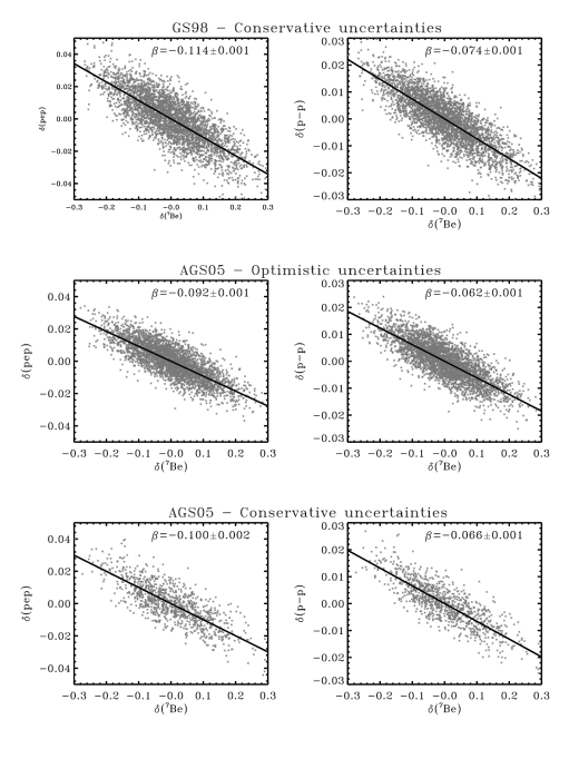
Figure 8: The pep vs. ⁷Be and the p-p vs. ⁷Be anti-correlations. The two fluxes are anti-correlated since only one p-p (or pep) neutrino is produced if hydrogen burning proceeds through the ³He(⁴He,$\gamma$)⁷Be reaction, whereas hydrogen burning in which ⁷Be is not involved creates two p-p neutrinos (or occasionally pep neutrinos).

The right hand panels of Figure 8 show the anti-correlation between the p-p and the ⁷Be neutrino fluxes. For the top right panel, GS98-Cons composition choice, the best-fit straight line has a slope

$$\beta({\rm pp,^{7}Be})~{}=~{}-0.0736\pm 0.0007\,.$$ (46)

The corresponding $1\sigma$ uncertainty in predicting $\delta({\rm pp})$ from a known value of the ⁷Be neutrino flux is

$$\sigma(\hbox{p-p};\,^{7}{\rm Be})~{}=~{}0.0054.$$ (47)

Thus one can predict the p-p flux to an accuracy of about 0.54% from a precisely measured value of the ⁷Be flux. The p-p versus ⁷Be anti-correlation is somewhat tighter than the pep versus ⁷Be anti-correlation.

Similar values are obtained for the other two cases. We find, respectively, $\beta({\rm pp,^{7}Be})~{}=~{}-0.0617\pm 0.0006$ and $\sigma(\hbox{p-p};\,^{7}{\rm Be})~{}=~{}0.0044$ and $\beta({\rm pp,^{7}Be})~{}=~{}-0.0659\pm 0.0014$ and $\sigma(\hbox{p-p};\,^{7}{\rm Be})~{}=~{}0.0046$ for the AGS05-Opt and AGS05-Cons cases respectively.

If one is interested in the inverse correlations, e.g. $\delta({\rm{}^{7}Be})=\beta({\rm{}^{7}Be,pep})\delta({\rm pep})$, they can be easily obtained by recalling that given two quantities $x$ and $y$, then if $x=\beta(x,y)\,y$ and $y=\beta(y,x)\,x$, where $\beta(x,y)$ and $\beta(y,x)$ are computed from least squares fitting, then they satisfy the relation

$$\beta(x,y)\beta(y,x)=\rho^{2}(x,y)$$ (48)

where $\rho(x,y)$ is the correlation coefficient between $x$ and $y$. The correlation coefficients of the neutrino fluxes are discussed in § 9 and summarized in Tables 16 and 17.

If our general picture of how nuclear fusion reactions occur in the solar interior is correct, then measurements of the pep (or p-p) and the ⁷Be neutrino fluxes must lie on one of the very similar lines shown in Figure 8. The values given in this subsection for $\beta({\rm pep,^{7}Be})$ represent a fundamental and testable prediction of the theory of nuclear energy generation in stars. They encapsulate the competition in the solar interior between the two primary branches, p-p(I) and p-p(II), of the p-p chain.

8.3.4 The pep vs. p-p Correlation

What is the relation between the production of the p-p and the pep neutrinos? They share the same nuclear matrix element and differ in a multiplicative factor that depends approximately upon the electron number density divided by the square root of the ambient temperature (Bahcall & May, 1969). This factor does not change very much from one solar model to the next. As a result, the pep rate is very nearly proportional to the p-p rate.

Suppose the pep flux is measured before the p-p flux is determined by a direct experiment. How accurately can one infer the p-p neutrino flux if one measures the pep flux? To answer this question, we plot $\delta({\rm pep})$ vs. $\delta(\hbox{p-p})$, where the meaning of the operator $\delta$ is defined in equation (39).

Figure 9 shows the rather-tight correlation between $\delta({\rm pep})$ and $\delta(\hbox{p-p})$. For the GS98-Cons case, the best-fit straight line of the form

$$\delta(\hbox{p-p})~{}=~{}\beta({\rm\hbox{p-p},pep})\delta({\rm pep})\,$$ (49)

has a slope

$$\beta({\rm\hbox{p-p,pep}})~{}=~{}0.586\pm 0.003\,,$$ (50)

and

$$\sigma(\hbox{p-p, pep})~{}=~{}0.0028\,.$$ (51)

Thus the p-p neutrino flux can be inferred from a precisely measured pep neutrino flux to an accuracy of about 0.3%. The results are similar for the other two cases we are considering. For the AGS05-Opt case, we find $\beta({\hbox{p-p,pep}})~{}=~{}0.642\pm 0.002$ and $\sigma(\hbox{p-p, pep})~{}=~{}0.0019$. Similarly, for AGS05-Cons we find $\beta({\hbox{p-p,pep}})~{}=~{}0.598\pm 0.007$ while $\sigma(\hbox{p-p, pep})~{}=~{}0.0027$.

Finally, we apply for the p-p vs. pep correlation the same reasoning leading to equation 44. Adopting a value for $\delta({\rm pep})=0.015$, the relative uncertainty in $\phi({\rm pp})$ due to the different values of $\beta({\hbox{p-p,pep}})$ that result from our two main simulations is only 0.1%.

In summary, the p-p flux can be inferred from a precisely measured pep flux to an accuracy of $0.25\%\pm 0.05\%$, depending upon which heavy element abundances are adopted and which abundance uncertainties are used. From the inverse correlation, the pep flux can be inferred from a precisely measured p-p flux to an accuracy of $0.39\%\pm 0.09\%$.

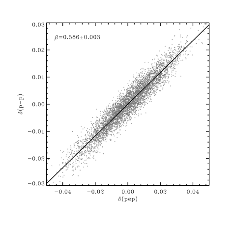
Figure 9: The correlation between the p-p and pep fluxes. The two fluxes are approximately proportional to each other since they share the same nuclear matrix element (Bahcall & May 1969).

8.4 The hep, ¹³N, ¹⁵O, and ¹⁷F Neutrino Fluxes

Figure 10: The hep, ¹³N, ¹⁵O and ¹⁷F neutrino fluxes from out Monte Carlo simulation with the GS98-Cons composition choice. The hep distribution follows a normal distribution with the parameters shown in the top-left panel. The distributions of the CNO fluxes are markedly asymmetric as they reflect the lognormal distribution for the composition uncertainties that is discussed in § 2.3. Results are analogous for the AGS05-Opt and AGS05-Cons composition choices.

Figure 10 shows, for GS98 abundances and conservative uncertainties, the histograms of the number of solar models with different values of the hep, ¹³N, ¹⁵O, and ¹⁷F solar neutrino fluxes. While the hep flux is normally distributed (99.9% C.L.), the 3 CNO fluxes follow lognormal distributions (better than 95% C.L.). The results for all three composition cases that we are considering are summarized in Tables 13, 14 and 15.

The total uncertainty for the hep neutrino flux is dominated by the 15.1% uncertainty (Park et al., 2003) from the calculation of the nuclear matrix element. All other sources of uncertainty contribute less than or of the order of 2%. Therefore, the calculated standard deviations for the hep neutrinos are essentially independent of the adopted heavy element abundances and their uncertainties.

For the ¹³N, ¹⁵O, and ¹⁷F solar neutrino fluxes, the standard deviations are dominated by composition uncertainties if we adopt conservative uncertainties. The marked asymmetry of the distributions of the CNO neutrino fluxes is apparent in Figure 10. This asymmetry reflects the lognormal distribution for composition uncertainties that we have adopted and discussed in § 2.3. If we use optimistic composition uncertainties, the cross section factor $S_{1,14}$ for the ¹⁴N(p,$\gamma$)¹⁵O reaction (8.4% uncertainty) and the composition uncertainties make comparable contributions to the ¹³N and ¹⁵O neutrino fluxes uncertainties.

There are no funded experiments for which the detection of the hep, ¹³N, ¹⁵O, and ¹⁷F solar neutrino fluxes seems likely if the fluxes and their uncertainties calculated in this paper are correct.

9 Neutrino Flux Correlation Coefficients

We have seen in § 8 that some of the neutrino fluxes are highly correlated. These correlations are exhibited in, for example, Figure 8, which illustrates the anti-correlation of the pep and pp fluxes with the ⁷Be flux, and Figure 9, which shows the correlation of the pep and the pp fluxes. These correlations play an important role in global analysis of solar neutrino experiments (see, e.g., Fogli & Lisi, 1995; Bahcall et al., 2001a; Fogli et al., 2002).

The correlations of the fluxes arise from two sources: 1) the solution of the equations of stellar evolution; and 2) the effects of changes in individual input parameters.

In the past, the correlations of solar neutrino fluxes have been taken into account by using the logarithmic partial derivatives of individual neutrino fluxes with respect to 9 input parameters (Bahcall & Ulrich, 1988; Bahcall, 1989). The standard treatment of the flux-correlations, when represented by partial derivatives of fluxes with respect to input parameters, is contained in the important paper by Fogli & Lisi (1995).

In this section, we use the results of our Monte Carlo simulations to derive the correlations due to all 21 input parameters and to the solution of the equations of stellar evolution. By directly calculating the correlation coefficients among the Monte Carlo neutrino fluxes, we are able to present a simple and complete summary of the correlations. These results will enable simpler and more accurate theoretical analysis of solar neutrino oscillations.

We summarize the correlations in terms of the correlation coefficients, $\rho(i,j)$, defined in the usual way by

$$\rho(i,j)~{}=~{}\frac{N^{-1}\sum_{n=1}^{N}\Delta\phi_{i}^{n}\Delta\phi_{j}^{n}}{\sigma_{i}\times\sigma_{j}}\,,$$ (52)

where $\Delta\phi_{i}^{n}=\phi_{i}^{n}-\phi_{i,{\rm average}}$, $\sigma_{i}$ is the standard deviation of the ith flux type ($i=$ pp, pep, hep, ⁷Be, ⁸B, ¹³N, ¹⁵O, and ¹⁷F), and $N=5,000$ is the total number of cases considered in the separate Monte Carlo simulations that incorporated GS98 or AGS05 heavy element abundances. The correlation matrix is symmetric, $\rho(i,j)~{}=~{}\rho(j,i)$, and has by definition unit diagonal elements.

Table 16: Correlation Coefficients for 5000 Sets of Neutrino Fluxes: Grevesse & Sauval (1998) Heavy Element Abundances and Conservative Uncertainties.

Flux	pp	pep	hep	7Be	8B	13N	15O	17F
pp	1.000	0.954	0.082	-0.819	-0.720	-0.349	-0.381	-0.319
pep	0.954	1.000	0.087	-0.780	-0.730	-0.407	-0.439	-0.369
hep	0.082	0.087	1.000	-0.062	-0.086	-0.052	-0.058	-0.076
7Be	-0.819	-0.780	-0.062	1.000	0.887	0.154	0.204	0.332
8B	-0.720	-0.730	-0.086	0.887	1.000	0.269	0.333	0.486
13N	-0.349	-0.407	-0.052	0.154	0.269	1.000	0.991	0.172
15O	-0.381	-0.439	-0.058	0.204	0.333	0.991	1.000	0.219
17F	-0.319	-0.369	-0.076	0.332	0.486	0.172	0.219	1.000

Table 16 and Table 17 present the correlation coefficients calculated with the Monte Carlo simulations that used, respectively, the Grevesse & Sauval (1998) heavy element abundances with conservative uncertainties and the Asplund et al. (2005) heavy element abundances with optimistic uncertainties.

We see from Table 16 and Table 17 that the pp and pep neutrino fluxes are strongly anti-correlated with the ⁷Be and ⁸B neutrino fluxes and mildly anti-correlated with the CNO neutrino fluxes. The pp and pep fluxes are, as discussed in § 8.3.4, very strongly correlated. The ⁷Be and ⁸B neutrino fluxes are strongly correlated, since both are initiated by the same fusion reaction, ³He(⁴He, $\gamma$)⁷Be. Since the ⁷Be and ⁸B fluxes both occur predominantly in higher temperature regions of the Sun (see Fig. 1), where the Gamow penetration factor is more easily overcome, these fluxes are also mildly correlated with the CNO neutrino fluxes that are also mostly produced at higher temperatures. Of course, the ¹³N and ¹⁵O neutrino fluxes are strongly correlated with each other since they are both involved in the CN cycle that operates close to steady-state in the inner ($R<0.12R_{\odot}$) regions of the Sun.

Comparing the correlation coefficients given in Table 16 and Table 17, we see that the same general trends are obtained independent of which assumption we make regarding the heavy element abundances and their uncertainties. However, there are important quantitative differences. In particular, the correlations involving the CNO neutrino fluxes with fluxes from the pp chain are weaker when the Asplund et al. (2005) abundances and optimistic uncertainties are adopted.

Table 17: Correlation Coefficients for Neutrino Fluxes: Asplund et al. (2005) Heavy Element Abundances and Optimistic Uncertainties.

Flux	pp	pep	hep	7Be	8B	13N	15O	17F
pp	1.000	0.967	-0.012	-0.796	-0.642	-0.127	-0.132	-0.111
pep	0.967	1.000	0.001	-0.793	-0.667	-0.162	-0.171	-0.137
hep	-0.012	0.001	1.000	0.022	0.021	-0.005	-0.008	-0.014
7Be	-0.796	-0.793	0.022	1.000	0.878	0.125	0.155	0.237
8B	-0.642	-0.667	0.021	0.878	1.000	0.257	0.296	0.412
13N	-0.127	-0.162	-0.005	0.125	0.257	1.000	0.984	0.299
15O	-0.132	-0.171	-0.008	0.155	0.296	0.984	1.000	0.338
17F	-0.111	-0.137	-0.014	0.237	0.412	0.299	0.338	1.000

10 Nuclear Fusion Fractions

For pedagogical purposes and in order to have a conceptual overview of solar energy generation, it is useful to calculate the fraction of the total nuclear energy generation that occurs via each of the most important fusion paths. We present in this section the best-estimates (given in the last column of Table 6 for the best current standard solar models) and the $1\sigma$ uncertainties in the best-estimates of the fractions that correspond to different ways of burning hydrogen.

Table 18 gives the fractions of the total nuclear fusion energy generation in standard solar models that are produced by different fusion reaction paths. We present results for all three of the composition options.

More than 99% of the total nuclear energy generation is produced by the p-p reactions in our solar models, while less than 1% of the energy is generated by the CNO reactions. These fractions are robust to all the input uncertainties of our standard solar models. The total standard deviations from variations in all the 21 input parameters in the Monte Carlo simulations are between 0.07% or 0.3%.

About 88% or 90% of the energy is derived, on average for our standard models, from reactions that begin with the fundamental p-p reaction and terminate with the ³He(³He, 2 p)⁴He reaction (p-p(I)). Nearly all of the remainder of the nuclear energy, 10% or 11%, is generated in our models by p-p reactions that go through the reaction ³He(⁴He, $\gamma$)⁷Be that creates ⁷Be solar neutrinos by electron capture (p-p(II)). These fractions also have relatively small variations (standard deviations) due to the choice of different input parameters. The standard deviations are typically 1% for the p-p(I) and p-p(II) fractions.

Extraordinary as it seems, most of solar neutrino astronomy so far has focused on the p-p(III) reactions that involve the production of rare ⁸B neutrinos. The crucial reaction sequence terminating these p-p reactions consists of the reaction ³He(⁴He,$\gamma$)⁷Be followed by ⁷Be(p,$\gamma$)⁸B. Less than 1% of the energy generation in our solar models corresponds to this rare reaction pathway and the standard deviation of this fraction is only about 0.1%. The Kamiokande (Fukuda et al., 1996), Super-Kamiokande (Fukuda et al., 2001, 2002), and SNO solar neutrino experiments (Ahmed et al., 2004; Aharmin et al., 2005) only detect neutrinos from this rare set of reactions. Moreover, the original chlorine solar neutrino experiment by R. Davis, Jr. and his colleagues (Cleveland et al., 1998) is primarily sensitive to ⁸B neutrinos because of a special superallowed transition between ³⁷Cl and ³⁷Ar (Bahcall, 1964).

Table 18: Fractions of Nuclear Energy Generation That Are Produced by Different Reaction Pathways

Fusion Branch	GS98-Cons	AGS05-Opt	AGS05-Cons
Fraction
pp	$99.2\pm 0.3$	$99.5\pm 0.1$	$99.5\pm 0.2$
CNO	$0.8\pm 0.2$	$0.5\pm 0.07$	$0.5\pm 0.1$
p-p(I)	$88.3\pm 1.3$	$89.6\pm 1.0$	$89.6\pm 1.1$
p-p(II)	$10.8\pm 1.1$	$9.6\pm 0.9$	$9.6\pm 1.0$
p-p(III)	$0.9\pm 0.1$	$0.8\pm 0.08$	$0.8\pm 0.08$

11 CONCLUSIONS AND DISCUSSION

We provide in this paper quantitative estimates of the accuracy with which standard solar models predict measurable quantities. These estimates provide the most comprehensive summary of solar model predictions and for many of the predicted quantities, e. g., the 8 helioseismologically measured quantities ($Y_{\rm surf}$, $R_{\rm CZ}$, and the 6 difference rms) the estimates given here provide the only consistent quantitative estimates of the uncertainties of the predictions.

As of this writing, there is considerable uncertainty regarding the best estimates for the surface chemical composition of the Sun, one of the important sets of input parameters for our Monte Carlo simulations. We have therefore carried out parallel sets of calculations for two very different sets of heavy element abundances: the Grevesse & Sauval (1998, GS98) abundances and the Asplund et al. (2005, AGS05) recommended abundances. We have used conservative estimates for the composition uncertainties together with the GS98 abundances and optimistic uncertainties together with the AGS05 abundances. Throughout this paper, and unless otherwise noted, we give without parentheses the results calculated with the GS98 abundances and conservative composition uncertainties and with parentheses the results calculated with AGS05 abundances and optimistic uncertainties.

Input Parameters and Their Uncertainties.

In § 2, we present and discuss the best-estimates and uncertainties for 19 important input parameters that are used in constructing the solar models that are considered in this paper. These parameters include nuclear fusion cross sections, the solar age and luminosity, the diffusion coefficient, and the 9 most important heavy element abundances on the surface of the Sun. Two additional input ’parameters’, the radiative opacity and the equation of state, are discussed separately in § 3. The opacity and the equation of state are complicated functions of the local conditions in the star and must therefore be treated in a different way than the single-valued input parameters discussed in § 2. For each standard solar model we simulate, all 21 input parameters are chosen from their separate probability distributions that are described in § 2 and § 3.

Standard Solar Models: 23 Predicted Quantities and Some Model Characteristics.

We present in § 5 the best-estimate predictions for 23 solar quantities that are either already measured or potentially measurable. These quantities include the 8 dominant neutrino fluxes, the event rates for the chlorine and gallium solar neutrino experiments, 8 quantities that have been determined precisely by helioseismological measurements, and 5 quantities (not all independent) that characterize the relative frequency of different nuclear fusion reactions in the Sun. We also summarize some of the main characteristics (not directly measurable) of the standard solar models, including the principal physical variables at the center of the Sun and at the base of the convective zone, as well as the initial composition. For the reader’s convenience, we also present compact tables of the profile of the solar sound speed and the density. Using quadratic interpolation, these tables can be used to reproduce precise values of the sound speed and density through the Sun. Finally, we present quantities that are useful in precise analysis of solar neutrino propagation, including the radial distribution of the production of the individual neutrino sources, as well as the electron and neutron number densities as a function of solar radius.

The Depth of the Convective Zone and the Surface Helium Abundance.

The measured depth of the solar convective zone is in good agreement with the predictions of standard solar models constructed with the GS98 heavy element abundances (see eq. 31). However, solar models constructed with the AGS05 recommended abundances and uncertainties (’optimistic uncertainties’) disagree with the measured depth of the solar convective zone by the equivalent of $3.9\sigma$ (see eq. 32). The strong disagreement goes away if we adopt ’conservative uncertainties’ for the heavy elements together with the AGS05 abundances (see eq. 33); this results because the optimistic uncertainties are large enough to reproduce a solar composition that resembles that of GS98.

The measured surface helium abundance is in very good agreement with solar models constructed with the GS98 heavy element abundances (see eq. 34). The agreement is poor, however, if AGS05 abundances are used: the discrepancy between measured and predicted surface helium abundance is $3.6\sigma$ (effective) if the AGS05 optimistic uncertainties are used and $2.8\sigma$ (effective) if conservative uncertainties are adopted (see eq. 35 and eq. 36). We conclude that the measured depth of the solar convective zone and the surface helium abundance both indicate that models constructed with the GS98 heavy element abundances are significantly closer to the actual Sun than are models constructed with the AGS05 recommended abundances. Figure 3 shows, for different assumed abundances and uncertainties, the distribution of solar models with different values of the depth of the convective zone and different values of the surface helium abundance.

Sound Speed and Density Profiles.

We present in § 7 the distributions of the sound speed and density difference rms. Table 12 gives the most probable values for the rms distributions and the respective uncertainties. The Monte Carlo simulation of models constructed with the GS98 composition have distributions strongly peaked very close to zero for all the six rms defined and used in this work. These distributions reflect a very good agreement between solar models constructed with the GS98 composition and results from helioseismology, reinforcing the conclusions drawn from the depth of the convective zone and surface helium abundance discussed above. The set of models constructed with the AGS05 composition, on the contrary, give rise to rms distributions that make evident the discrepancy in the sound speed and density profiles introduced by the adoption of the AGS05 composition. In addition, Figures 4 and 5 allow us to conclude that the uncertainties in all the other input parameters entering a standard solar model cannot compensate for the degradation introduced by the new recommended set of solar abundances.

The Predicted Solar Neutrino Fluxes.

We analyze in § 8 the calculated distributions of solar neutrino fluxes. Table 15 gives the total $1\sigma$ uncertainty for each neutrino source and for all three choices of heavy element composition and their uncertainties. The results are in very good agreement with the uncertainties estimated using power-law dependences of the fluxes as a function of input parameters. The distribution of calculated fluxes for each neutrino source is well described by either a normal or a lognormal distribution, depending on what is the dominant source of uncertainty, with the tabulated standard deviation.

The calculated ⁸B solar neutrino flux is in good agreement with the value measured by solar neutrino experiments. The theoretical uncertainty in the prediction of the ⁸B neutrino flux (11% to 17%, depending upon the choice of heavy element composition and uncertainties) is larger than the uncertainty (5%) in the experimental determination. For all other solar neutrino sources, the experimental uncertainties greatly exceed the solar model uncertainties.

The ⁷Be solar neutrino flux will be measured in the next few years. The solar model uncertainties in the prediction of the ⁷Be neutrino flux vary from 9.3% to 10.5% depending upon the choice of heavy element abundances and their uncertainties. It is possible that the pep neutrino flux will be measured in one of the same experiments as the ⁷Be neutrino flux. The predicted anti-correlation between the pep and ⁷Be neutrino fluxes is given in eq. (40) and eq. (41) and is shown in figure 8.

The solar model predictions for the p-p and the pep neutrino fluxes are strongly correlated with each other and the p-p neutrino flux is anti-correlated with the ⁷Be neutrino flux. These relations between the predicted neutrino fluxes represent important testable predictions of the solar models and are discussed and analyzed quantitatively in § 8.

The Correlation Coefficients of the Neutrino Fluxes.

The correlations between the different neutrino fluxes are succinctly summarized by the matrix of correlation coefficients. Table 16 and Table 17 present the correlation coefficients of the neutrino fluxes for, respectively, GS98 heavy element abundances and conservative uncertainties and AGS05 heavy element abundances and optimistic uncertainties. These correlation coefficients can be used to make a more constrained and precise analysis of solar neutrino oscillations.

Nuclear Energy Generation Pathways.

Table 18 summarizes the calculated fraction of the total nuclear energy generation that is produced by different nuclear fusion pathways. For all choices of the surface heavy element abundances and their uncertainties, the p-p chain is responsible for more than 99% of the total energy generation. The estimated uncertainty in the p-p energy generation fraction is less than or of order 0.2%. The CNO energy fraction is less than 1%. About 88% to 90% of the p-p energy generation is from reactions that are terminated by the ³He(³He, 2p)⁴He reaction with an uncertainty of about 1%. Although most of solar neutrino astronomy has so far been focused on the high energy ⁸B neutrinos, the nuclear fusion reactions that lead to the production of ⁸B represent less than 1% of the total solar energy generation (best-estimate varies from 0.81% to 0.91% with an uncertainty of only 0.08%).

Future solar neutrino experiments that measure different solar neutrino fluxes can determine empirically the nuclear energy generation fractions and test the solar model predictions given in Table 18.

J. N. B. and A. M. S. were supported in part by NSF grants PHY-0070928 and PHY-0503584 to the Institute for Advanced Study. A.M.S. was also supported by the W. M. Keck Foundation through a grant-in-aid to the Institute for Advanced Study. S. B. was partially supported by NSF grants ATM-0206130 and ATM-0348837. This work utilizes data from the Solar Oscillations Investigation / Michelson Doppler Imager (SOI/MDI) on the Solar Heliospheric Observatory (SOHO). The MDI project is supported by NASA grant NAG5-8878 to Stanford University. SOHO is a project of international cooperation between ESA and NASA. We are grateful to M. Chen, P. Goldreich, E. Lisi, A. McDonald, M. Pinsonneault, and S. Tremaine, and particularly to C. Peña-Garay for valuable comments, discussions, and suggestions during the extended period in which this project was carried out and the results analyzed. Computations presented in this paper were done with the Scheides Beowulf cluster at the Institute for Advanced Study.

Appendix A Lognormal distribution

We briefly summarize some important properties of lognormal probability distribution functions used in this work. We also define the $1\sigma$ confidence level interval we have adopted throughout this paper when a given quantity is lognormally distributed.

A random variable $x$ is lognormally distributed when its probability density function $f(x)$ is given by

$$f(x)=\left[s\sqrt{2\pi}(x-\theta)\right]^{-1}\exp{\left[-\frac{(\log{(x-\theta)}-m)^{2}}{2s^{2}}\right]}.$$ (A1)

Here, $m$ and $s$ are the scale and shape parameters respectively. $\theta$ is the location parameter which we assume equal to 0 for simplicity. The most probable value (mode) and the mean values of a lognormally distributed quantity, respectively, are

$$Q=\exp{(m-s^{2})}\ \ \ ;\ \ \ \ \ \ \mu=\exp{(m+s^{2}/2)}.$$ (A2)

In general, we adopt as the $1\sigma$ confidence level interval that given by the limits of the integral

$$\int^{x_{+}}_{x_{-}}f(x)\,dx=0.683,\ \ \ \ {\rm with}\ f(x_{-})=f(x_{+}).$$ (A3)

Equation A3 uniquely defines the $1\sigma$ confidence level interval $\left[x_{-},x_{+}\right]$. An interesting relation between $x_{-}$ and $x_{+}$ is

$$x_{-}x_{+}=Q^{2}.$$ (A4)

The $1\sigma$ confidence level interval is conveniently expressed with respect to the mode $Q$ by introducing the quantities $\sigma_{+}$ and $\sigma_{-}$ defined by

$$\sigma_{+}=x_{+}-Q\ \ \ \ \ \ \sigma_{-}=Q-x_{-}.$$ (A5)

When relative values for $\sigma_{+}$ or $\sigma_{-}$ are quoted in this paper, they are effectively calculated as $\sigma_{+}/Q$ and $\sigma_{-}/Q$.

In practice, for a given dataset $\left\{x_{i}\right\}_{i=1}^{N}$, $m$ and $s$ are estimated as

$$m=N^{-1}\sum_{i=1}^{N}\log{x_{i}}$$ (A6)

and

$$s^{2}=(N-1)^{-1}\sum_{i=1}^{N}(\log{x_{i}}-m)^{2}\,.$$ (A7)

References

- Abdurashitov et al. (2002) Abdurashitov, J. N., et al. (SAGE Collaboration) 2002, J. Exp. Theor. Phys., 95, 181
- Abdurashitov et al. (2003) Abdurashitov, J. N., et al. (SAGE Collaboration) 2003, Nucl. Phys. B (Proc. Suppl.), 118, 39
- Adelberger et al. (1998) Adelberger, E. G., et al. 1998, Rev. Mod. Phys., 70, 1265
- Aharmin et al. (2005) Aharmim, B., et al. (SNO Collaboration), preprint (nucl-ex/0502021)
- Ahmed et al. (2004) Ahmed, S. N., et al. (SNO Collaboration) 2004, Phys. Rev. Lett., 92, 181301
- Alexander & Ferguson (1994) Alexander, D. R., & Ferguson, J. W. 1994, ApJ 437, 879
- Alimonti et al. (2002) Alimonti, G., et al. (BOREXINO Collaboration) 2002, Astropart. Phys., 16, 205
- Allende Prieto et al. (2001) Allende Prieto, C., Lambert, D. L., & Asplund, M. 2001, ApJ, 556, L63
- Allende Prieto et al. (2002) Allende Prieto, C., Lambert, D. L., & Asplund, M. 2002, ApJ, 573, L137
- Altmann et al. (2005) Altmann, G., et al. (GNO collaboration) 2005, Phys. Lett. B, 616, 174
- Angulo & Descouvemont (2001) Angulo C., & Descouvemont, P. 2001, Nuc. Phys. A, 4, 755
- Antia & Basu (2005) Antia, M., & Basu, S. 2005, ApJ, 620, L129
- Araki et al. (2005) Araki, T., et al. (KamLAND collaboration) 2005, Phys. Rev. Lett., 94, 081801
- Asplund (2000) Asplund, M. 2000, A&A, 359, 755
- Asplund et al. (2005) Asplund, M., Grevesse, N., & Sauval, A. J. 2005, in ASP Conf. Ser. 336, Cosmic Abundances as Records of Stellar Evolution and Nucleosynthesis, ed. T. G. Barnes III, & F. N. Bash (San Francisco: ASP), 25
- Asplund et al. (2004) Asplund, M., Grevesse, N., Sauval, A. J., Allende Prieto, C., & Kiselman, D. 2004, A&A, 417, 751
- Asplund et al. (2000) Asplund, M., Nordlund, A., Trampedach, R., & Stein, R. F. 2000, A&A, 359, 743
- Badnell et al. (2005) Badnell, N. R., Bautista, M. A., Butler, K., Delahaye, F., Mendoza, C., Palmeri, P., Zeippen, C. J., & Seaton, M. J. 2005, MNRAS, 360, 458
- Bahcall (1964) Bahcall, J. N. 1964, Phys. Rev. Lett., 12, 300
- Bahcall (1989) Bahcall, J. N. 1989, Neutrino Astrophysics (Cambridge: Cambridge University Press)
- Bahcall (1994) Bahcall, J. N. 1994, Phys. Rev. D, 49, 3923
- Bahcall (1997) Bahcall, J. N. 1997, Phys. Rev. C 56, 3391
- Bahcall (2002) Bahcall, J. N. 2002, Phys. Rev. C, 65, 025801
- Bahcall et al. (1968) Bahcall, J. N., Bahcall, N. A., & Shaviv, G. 1968, Phys. Rev. Lett,. 20, 1209
- Bahcall et al. (2005a) Bahcall, J. N., Basu, S., Pinsonneault, M. H., & Serenelli, A. M. 2005a, ApJ, 618, 1049
- Bahcall et al. (2005c) Bahcall, J. N., Basu, S., & Serenelli, A. M. 2005c, ApJ, 631, 1281
- Bahcall et al. (2004a) Bahcall, J. N., Gonzalez-Garcia, M. C., & Peña-Garay, C. 2004a, J. High Energy Phys., 08, 016
- Bahcall et al. (2001a) Bahcall, J. N., Krastev, P. I., & Smirnov, A. Yu. 2001a, Phys. Rev. D, 63, 053012
- Bahcall & May (1969) Bahcall, J. N., & May, R. M. 1969, ApJ, 155, 501
- Bahcall & Pinsonneault (1995) Bahcall, J. N., & Pinsonneault, M. H. 1995, Rev. Mod. Phys., 67, 781
- Bahcall & Pinsonneault (2004) Bahcall, J. N., & Pinsonneault, M. H. 2004, Phys. Rev. Lett., 92, 121301
- Bahcall et al. (2001b) Bahcall, J. N., Pinsonneault, M. H., & Basu, S. 2001b, ApJ, 555, 990
- Bahcall et al. (1997) Bahcall, J. N., Pinsonneault, M. H., Basu, S. & Christensen-Dalsgaard, J. 1997, Phys. Rev. Lett., 78, 171
- Bahcall & Serenelli (2005) Bahcall, J. N., & Serenelli, A. M. 2005, ApJ 626, 530
- Bahcall et al. (2005b) Bahcall, J. N., Serenelli, A.M., & Basu, S. 2005b, ApJ, 621, L85
- Bahcall et al. (2004b) Bahcall, J. N., Serenelli, A. M., & Pinsonneault, M. H. 2004b, ApJ, 614, 464
- Bahcall & Ulrich (1988) Bahcall, J. N., & Ulrich, R. K. 1988, Rev. Mod. Phys., 60, 297
- Barger et al. (1991) Barger, V., Deshpande, N., Pal, P. B., Phillips, R. J. N., & Whisnant, K. 1991, Phys. Rev. D, 43, R1759
- Basu (1998) Basu, S. 1998, MNRAS, 298, 719
- Basu (2002) Basu, S. 2002, in Proc. SOHO 11 Symp., From Solar Min to Solar Max: Half a Solar Cycle with SOHO, ed. A. Wilson (ESA SP-508; Noordwijk: ESA), 7
- Basu & Antia (1997) Basu, S., & Antia, H. M. 1997, MNRAS, 287, 189
- Basu & Antia (2004) Basu, S., & Antia, H. M. 2004, ApJ, 606, L85
- Basu et al. (2000) Basu, S., Bahcall, J. N., & Pinsonneault, M. H. 2000, ApJ, 529, 1084
- Bertello et al. (2000) Bertello, L., et al. 2000, ApJ, 535, 1066
- Cleveland et al. (1998) Cleveland, B. T., Daily, T., Davis, R., Jr., Distel, J. R., Lande, K., Lee, C. K., Wildenhain, P. S., & Ullman, J. 1998, ApJ, 496, 505
- Christensen-Dalsgaard et al. (1991) Christensen-Dalsgaard, J., Gough, D. O., & Thompson, M. J. 1991, ApJ, 378, 413
- Davis et al. (1968) Davis, R. Jr., Harmer, D. S., & Hoffmann, K. C. 1968, Phys. Rev. Lett. 20, 1205
- Dolbeau et al. (2005) Dolbeau, J., Giomataris, I., Gorodetzky, P., Patzak, T., Salin, P., & Sarat, A. 2005, Nucl. Phys. B (Proc. Suppl.), 138, 94
- Ejiri et al. (2000) Ejiri, H., Engel, J., Hazama, R., Krastev, P., Kudomi, N., & Robertson, R. G. H. 2000, Phys. Rev. Lett., 85, 2917
- Ferguson et al. (2005) Ferguson, J. W., Alexander, D. R., Allard, F., Barman, T., Bodnarik, J. G., Hauschildt, P. H., Heffner-Wong, A., & Tamanai, A. 2005, ApJ, 623, 585
- Fogli & Lisi (1995) Fogli, G. L., & Lisi, E. 1995, Astropart. Phys., 3, 185
- Fogli et al. (2002) Fogli, G. L., Lisi, E., Marrone, A., Montanino, D., & Palazzo, A. 2002, Phys. Rev. D, 66, 053010
- Formicola et al. (2004) Formicola, A., et al. 2004, Phys. Lett. B, 591, 61
- Freedman & Kayser (2004) Freedman, S. J., & Kayser, B. (co-chairs of the organizing committee), prepared by the members of the APS Multidivisional Neutrino Study (physics/0411216)
- Friedland et al. (2004) Friedland, A., Lunardini, C., & Peña-Garay, C. 2004, Phys. Lett. B, 594, 347
- Fröhlich & Lean (1998) Fröhlich, C., & Lean, J. 1998, Geophys. Res. Lett., 25, 4377
- Fukuda et al. (2001) Fukuda, S., et al. (Super-Kamiokande Collaboration) 2001, Phys. Rev. Lett., 86, 5651
- Fukuda et al. (2002) Fukuda, S., et al. (Super-Kamiokande Collaboration) 2002, Phys. Lett. B, 539, 179
- Fukuda et al. (1996) Fukuda, Y., et al. (Kamiokande Collaboration) 1996, Phys. Rev. Lett., 77, 1683
- Galbiati et al. (2005) Galbiati, C., Pocar, A., Franco, D., Ianni, A., Cadonati, L., & Schönert, A., 2005, Phys. Rev. C, 71, 055805
- Gorodetsky et al. (1999) Gorodetsky, P., Patzak, T., Seguinot, J., Vanel, J. C., Ypsilantis, T., Derre, J., Giomataris, I., & Zaccone, H. 1999, Nucl. Inst. Meth. A, 433, 554
- Grevesse (1984) Grevesse, N. 1984, Phys. Scr., 8, 49
- Grevesse & Sauval (1998) Grevesse, N., & Sauval, A. J. 1998, Space Sci. Rev., 85, 161
- Gribov & Pontecorvo (1969) Gribov, V. N., & Pontecorvo, B. M. 1969, Phys. Lett. B, 28, 493
- Gruzinov & Bahcall (1997) Gruzinov, A. V., & Bahcall, J. N. 1997, ApJ, 490, 437
- Guzik & Cox (1993) Guzik, J. A., & Cox, A. N. 1993, ApJ, 411, 394
- Guzik & Watson (2004) Guzik, J., & Watson, L. W. 2004, in the Proc. of the SOHO 14th-GONG 2004 Workshop, Yale University, 12-16th July 2004, ed. D. Dansey, ESA SP-559, 456
- Guzik et al. (2005) Guzik, J. A., Watson, L. W., & Cox, A. N. 2005, ApJ, 627, 1049
- Hampel et al. (1999) Hampel, W., et al. (GALLEX collaboration) 1999, Phys. Lett. B, 447, 127
- Iglesias & Rogers (1996) Iglesias, C. A., & Rogers, F. J. 1996, ApJ, 464, 943
- Junghans et al. (2003) Junghans, A. R., et al. 2003, Phys. Rev. C, 68, 065803
- Junker (1998) Junker, M., et al. 1998, Phys. Rev. C, 57, 2700
- Kosovichev & Fedorova (1991) Kosovichev, A. G., & Fedorova, A. V. 1991, Sov. Astron., 35, 507
- Lanou (2005) Lanou, R. E. (for the HERON Group) 2005, Nucl. Phys. B (Proc. Suppl.), 138, 98
- Lim & Marciano (1988) Lim, C. S., & Marciano, W. 1988, Phys. Rev. D, 37, 1368
- Lodders (2003) Lodders, K. 2003, ApJ, 591, 1220
- McDonald (2004) McDonald, A. B. 2004, New J. Phys., 6, 121
- McKinsey & Coakley (2005) McKinsey, D. N., & K. J. Coakley, K. J. 2005, Astropart. Phys., 22, 355
- McKinsey & Doyle (2000) McKinsey, D. N., & Doyle, J. M. 2000, J. Low Temp. Phys., 118, 153
- Mikheyev & Smirnov (1985) Mikheyev, S. P., & Smirnov, A. Y. 1985, Soviet J. Nucl. Phys., 42, 913
- Mikheyev & Smirnov (1986) Mikheyev, S. P., & Smirnov, A. Yu. 1986, in ‘86 Massive Neutrinos in Astrophysics and in Particle Physics, Proc. of the Sixth Moriond Workshop, ed. O. Fackler, & Trân Thanh Vân (Gif-sur-Yvette: Editions Frontières), 355
- Montalban et al. (2004) Montalbán, J., Miglio, A., Noels, A., Grevesse, N., & di Mauro, M. P. 2004, in the Proc. SOHO14/GONG2004 Workshop, Helio and Astroseismology: Towards a Golden Future, ed. D. Dansey, ESA SP-559, 574, astro-ph/0408055, v2
- Mukhamedzhanov et al. (2003) Mukhamedzhanov, A. M., et al. 2003, Phys. Rev. C, 67, 065804
- Nakahata (2001) Nakahata, M. 2001, in Proceedings of the Third International Workshop on Neutrino Oscillations and Their Origin (NOON2001), ed. Y. Suzuki, M. Nakahata, Y. Fukuda, Y. Takeuchi, T. Mori, & T.Yoshida (Singapore: World Scientific), 92
- Nara Singh et al. (2004) Nara Singh, B. S., Hass, M., Nir-El, Y., & Haquin, G. 2004, Phys. Rev. Lett., 93, 262503
- Oberauer et al. (2005) Oberauer, L., von Feilitzsch, F., & Potzel, W. 2005, Nucl. Phys. B (Proc. Suppl.), 138, 108
- Park et al. (2003) Park, T. S., et al. 2003, Phys. Rev. C, 67, 055206
- Pijpers & Thompson (1992) Pijpers, F. P., & Thompson, M. J. 1992, A&A, 262, L33
- Pijpers & Thompson (1994) Pijpers, F. P., & Thompson, M. J. 1994, A&A, 281, 231
- Proffitt (1994) Proffitt, C. R. 1994, 425, 849
- Rabello-Soares, et al. (1999) Rabello-Soares, M. C., Basu, S., & Christensen-Dalsgaard, J. 1999, MNRAS, 309, 35
- Raghavan (1976) Raghavan, R. S. 1976, Phys. Rev. Lett. 37, 259
- Raghavan (2001) Raghavan, R. S., unpublished (hep-ex/0106054)
- Rogers (2001) Rogers, F. J. 2001, Contrib. Plasma Phys., 41, 179
- Rogers et al. (1996) Rogers, F. J., Swenson, F. J., & Iglesias, C. A. 1996, ApJ, 456, 902
- Runkle et al. (2005) Runkle, R. C., et al. 2005, Phys. Rev. Lett., 94, 082503
- Schou et al. (1998) Schou, J., Christensen-Dalsgaard, J., Howe, R., Larsen, R. M., Thompson, M. J., & Toomre, J. 1998, in Structure and Dynamics of the Interior of the Sun and Sun-like Stars, ed. S. G. Korzennik & A. Wilson (ESA SP-418; Noordwijk: ESA), 845
- Seaton (2005) Seaton, M. J. 2005, MNRAS, 362, L1
- Seaton & Badnell (2004) Seaton, M. J., & Badnell, N. R. 2004, MNRAS, 354, 457
- Spiro & Vignaud (1990) Spiro, M., & Vignaud, D. 1990, Phys. Lett. B, 242, 279
- Suzuki (2005) Suzuki, Y. 2005, Nucl. Phys. B (Proc. Suppl.), 143, 27
- Suzuki et al. (2000) Suzuki, Y., et al. 2000, preprint (hep-ph/0008296)
- Thoul et al. (1994) Thoul, A. A., Bahcall, J. N., & Loeb, A. 1994, ApJ, 421, 828
- Turck-Chièze et al. (2004) Turck-Chièze, S., Couvidat, S., Piau, L., Ferguson, J., Lambert, P., Ballot, J., García, R. A. & Nghiem, P. 2004, Phys. Rev. Lett., 93, 211102
- Weiss & Schlattl (2000) Weiss, A., & Schlattl, H. 2000, A&AS, 144, 487
- Wolfenstein (1978) Wolfenstein, L. 1978, Phys. Rev. D, 17, 2369