Scalar statistics on the sphere: application to the CMB

Abstract

A method to compute several scalar quantities of Cosmic Microwave Background maps on the sphere is presented. We consider here four type of scalars: the Hessian matrix scalars, the distortion scalars, the gradient related scalars and the curvature scalars. Such quantities are obtained directly from the spherical harmonic coefficients $a_{\ell m}$ of the map. We also study the probability density function of these quantities for the case of a homogeneous and isotropic Gaussian field, which are functions of the power spectrum of the initial field. From these scalars it is posible to construct a new set of scalars which are independent of the power spectrum of the field. We test our results using simulations and find a good agreement between the theoretical probability density functions and those obtained from simulations. Therefore, these quantities are proposed to investigate the presence of non-Gaussian features in CMB maps. Finally, we show how to compute the scalars in presence of anisotropic noise and realistic masks.

1 Introduction

The Cosmic Microwave Background (CMB) is currently one of the most valuable tools of cosmology, providing with a great wealth of information about the universe. A particularly interesting subject is whether the CMB temperature fluctuations follow or not a Gaussian distribution. This is a key issue since Gaussian fluctuations are predicted by the standard inflationary theory, whereas alternative theories produce non-Gaussian signatures in the CMB. In addition, foregrounds and systematics may also introduce non-Gaussianity, which should be carefully studied in order to avoid its misidentification with intrinsic non-Gaussian fluctuations.

A large effort has been recently devoted to the study of the Gaussian character of the CMB using the multi-frequency all-sky CMB data provided by the WMAP satellite of NASA (Bennett et al. 2003a), finding, in some cases, unexpected results. Some authors have found that the WMAP data are consistent with Gaussianity using different types of analysis (Komatsu et al. 2003, Colley & Gott 2003, Gaztañaga & Wagg 2003, Gaztañaga et al. 2003). However, other studies have produced a positive detection of non-Gaussianity and/or have shown north-south asymmetries (Chiang et al. 2003, Eriksen et al. 2004a,b, Park 2004, Copi et al. 2004, Vielva et al. 2004, Hansen et al. 2004, Mukherjee & Wang 2004, Land & Magueijo 2004, Hansen et al. 2004, Larson & Wandelt 2004, McEwen et al. 2004, Cruz et al. 2005). Although some of these results could be explained by the presence of foreground contamination, in other cases the origin of the detection is uncertain and a primordial origin can not be discarded. These results motivates, even more, the development of novel techniques to perform further Gaussianity analyses of the CMB.

In this paper we have focused on the study of several scalar quantities constructed from the derivatives of the CMB field on the sphere. In particular, we have considered the modulus of the gradient, the Laplacian, the distortion, the shear, the ellipticity, the shape index, the eigenvalues of the negative Hessian matrix, the Gaussian curvature and the derivative of the squared modulus of the gradient. A procedure to calculate the scalars directly from the $a_{\ell m}$ harmonic coefficients is provided. In addition, we have obtained expressions for the probability distributions of the previous quantities for the case of a homogeneous and isotropic Gaussian random field (HIGRF), which depend on the power spectrum of the initial field. In order to remove this dependence, we have also constructed a new set of normalized scalars whose probability distribution is independent of the power spectrum.

A number of works have been already devoted to the study of some of these or other related quantities. Also, some of them have been applied to study the Gaussianity of the WMAP data, providing interesting results. In a pioneering work, Bond & Efstathiou (1987) studied different statistical properties of the CMB, assuming a 2-dimensional Gaussian field, which included the number densities of hot and cold spots, the eccentricities of peaks and peak correlation properties. Barreiro et al. (1997) studied also the mean number of maxima and the probability distribution of the Gaussian curvature and the eccentricity of peaks of the CMB for different shapes of the power spectra. Wandelt, Hivon & Górski (1998) developed efficient algorithms for fast extrema search as well as for the simulation of the gradient vector and the curvature tensor fields on the sphere associated to the temperature field. The power to detect non-Gaussianity in the CMB of the number, eccentricity and Gaussian curvature of excursion sets above (and below) a threshold was tested by Barreiro, Martínez-González & Sanz (2001) using Gaussian and non-Gaussian simulations, finding that the Gaussian curvature was the best discriminator. Doré, Colombi & Bouchet (2003) tested the power of a technique based on the proportion of hill, lake and saddle points (which are defined attending to their local curvature) on flat patches of the sky. A study of the ellipticity of the CMB was performed for the COBE-DMR (Gurzadyan & Torres 1997) and Boomerang data (Gurzadyan et al. 2003), which seemed to indicate a slight excess of ellipticity for the largest spots with respect to what was expected in the standard model. These results were recently confirmed by repeating the analysis on the WMAP data using the same region of the sky observed by Boomerang (Gurzadyan et al. 2004). Eriksen et al. (2004b) applied the Minkowski functionals and the length of the skeleton (Novikov, Colombi & Doré 2003) to the WMAP data finding evidence of non-Gaussianity and asymmetry between the northern and southern hemispheres. The length of the skeleton is a quantity defined in terms of the first and second derivatives of the field and the previous work provided with an algorithm to calculate it on the sphere for a CMB map in HEALPix pixelization. Hansen et al. (2004) found north/south asymmetries on the WMAP data using the local curvature, which were consistent with the results of Eriksen et al. (2004b). Finally, Cabella et al. (2004) used a method based on the local curvature to constrain the value of the non-linear coupling constant $f_{\rm NL}$ from the WMAP data.

The paper is organised as follows. In $\S$2 we introduce the different considered scalars and describe how to calculate them from the covariant derivatives of a 2D field and, in particular, for spherical coordinates. In $\S$3 we obtain analytical (or semi-analytical) expressions for the probability density function (pdf) of the considered scalars for a homogeneous and isotropic Gaussian field on the sphere. In $\S$4 we construct a new set of related scalars which are independent of the power spectrum of the field and we obtain their theoretical distribution functions for the Gaussian case. The theoretical results are also compared with CMB simulations. $\S$5 shows how to deal with more realistic simulations, including anisotropic noise and a mask that covers the Galactic plane and the point sources. In $\S$6 we present our conclusions and outline future applications of this work. Appendix A gives the expressions necessary to calculate the derivatives of the field from the $a_{\ell m}$ coefficients. In Appendix B we present some useful results regarding spherical harmonic series. Finally, Appendix C gives some guidelines on how to deduce the distribution functions of ordinary and normalised scalars.

2 Scalars on the sphere

Let us consider a 2-dimensional field T$(x_{1},x_{2})$. From the field derivatives we can construct quantities that are scalars under a change of the coordinate system (i. e. regular general transformation $(x_{1},x_{2})\to(x_{1}^{\prime},x_{2}^{\prime})$: $s^{\prime}(x_{1}^{\prime},x_{2}^{\prime})=s(x_{1},x_{2})$). Regarding 1st derivatives, a single scalar can be constructed in terms of the ordinary derivative $T_{,i}$. Regarding 2nd covariant derivatives, $T_{;ij}$, of T$(x_{1},x_{2})$ can be expressed as a function of the ordinary derivatives $T_{,ij}$ and the Christoffel symbols $\Gamma_{ij}^{k}$ as follows

$$T_{;ij}=T_{,ij}-\Gamma_{ij}^{k}T_{,k}$$ (1)

To construct linear scalars we need to contract the indices of these covariant tensorial quantities.

The scalars that depend on second derivatives, although can be expressed as functions of the covariant derivatives, are usually defined in terms of the eigenvalues $\lambda_{1},\lambda_{2}$, of the negative Hessian matrix $A$ of the field T$(x_{1},x_{2})$

$$A=\left(-T_{;ij}\right).$$ (2)

That is, $\lambda_{1}$ and $\lambda_{2}$ are the (negative) second derivatives along the two principal directions. In the following we will assume $\lambda_{1}>\lambda_{2}$.

Taking into account the values of $\lambda_{1}$, $\lambda_{2}$, we can distinguish among three type of points (e. g. Doré et al. 2003): hill (both eigenvalues are positive), lake (both are negative) and saddle ($\lambda_{1}>0,\lambda_{2}<0$). We will also distinguish between saddle points with $|\lambda_{1}|>|\lambda_{2}|$, that we will call saddle_-, and those with $|\lambda_{1}|<|\lambda_{2}|$, saddle₊ (the sign +,- refers to the sign of the Laplacian, see below).

Hereinafter, we will consider spherical coordinates $(\theta,\phi)$, for which the metric is given by

$$ds^{2}=d\theta^{2}+\sin^{2}\theta~{}d\phi^{2}~{},$$ (3)

which gives the following non-zero Christoffel symbols:

$$\Gamma_{\phi\theta}^{\phi}=\Gamma_{\theta\phi}^{\phi}=\frac{\cos\theta}{\sin\theta},~{}~{}~{}~{}\Gamma_{\phi\phi}^{\theta}=-\sin\theta\cos\theta~{}.$$ (4)

It is convenient to define the following quantities for the spherical case:

$$p=\left[T^{,\theta}T_{,\theta}\right]^{\frac{1}{2}}=\frac{\partial T}{\partial\theta}~{},$$ (5)

$$q=\left[T^{,\phi}T_{,\phi}\right]^{\frac{1}{2}}=\frac{1}{\sin\theta}\frac{\partial T}{\partial\phi}~{},$$ (6)

$$r=\left[T_{\ \ \theta}^{;\theta}T_{\ \ \theta}^{;\theta}\right]^{\frac{1}{2}}=\frac{\partial^{2}T}{\partial\theta^{2}}~{},$$ (7)

$$s=\left[T_{\ \ \phi}^{;\phi}T_{\ \ \phi}^{;\phi}\right]^{\frac{1}{2}}=\frac{1}{\sin^{2}\theta}\frac{\partial^{2}T}{\partial\phi^{2}}+\frac{\cos\theta}{\sin\theta}\frac{\partial T}{\partial\theta}~{},$$ (8)

$$t=\left[T_{\ \ \theta}^{;\phi}T_{\ \ \phi}^{;\theta}\right]^{\frac{1}{2}}=\frac{1}{\sin\theta}\frac{\partial^{2}T}{\partial\theta\partial\phi}-\frac{\cos\theta}{\sin^{2}\theta}\frac{\partial T}{\partial\phi}~{}.$$ (9)

We will express all the scalars as a function of these five quantities. All of them, and therefore the scalars, can be easily computed from the $a_{\ell m}$ coefficients of the field (see Appendix A).

In the following, we present some of these scalars as function of the covariant derivatives. We will also relate them to the former defined quantities for the spherical case.

Note that, although we are considering the spherical case, the expressions given for the scalars as a function of the covariant derivatives are valid for any 2-dimensional surface. In particular, if observing a small portion of the sky, we can assume that we have a flat patch. In this case, the scalars can be easily obtained taking into account that all the Christoffel symbols are zero.

2.1 The Hessian matrix scalars

We include in this section the algebraical quantities related to the Hessian matrix: eigenvalues, trace and determinant.

2.1.1 The eigenvalues

The eigenvalues of the negative Hessian matrix are scalars of the field T, and they can be expressed as follows

$$2\lambda_{1}=-\left(T_{\ \ i}^{;i}\right)+\sqrt{\left(T_{\ \ i}^{;i}\right)^{2}-2\left(T_{\ \ i}^{;i}T_{\ \ j}^{;j}-T_{\ \ i}^{;j}T_{\ \ j}^{;i}\right)}~{},$$ (10)

$$2\lambda_{2}=-\left(T_{\ \ i}^{;i}\right)-\sqrt{\left(T_{\ \ i}^{;i}\right)^{2}-2\left(T_{\ \ i}^{;i}T_{\ \ j}^{;j}-T_{\ \ i}^{;j}T_{\ \ j}^{;i}\right)}~{}.$$ (11)

For the spherical coordinate system, we can rewrite them in the following way:

$$2\lambda_{1}=-\left(r+s\right)+\sqrt{(r-s)^{2}+(2t)^{2}}~{},$$ (12)

$$2\lambda_{2}=-\left(r+s\right)-\sqrt{\left(r-s\right)^{2}+\left(2t\right)^{2}}~{}.$$ (13)

Note that $\lambda_{1}\geq\lambda_{2}$. Therefore for values of $\lambda_{2}>0$ we have hill points whereas values of $\lambda_{1}<0$ correspond to lake points. These eigenvalues coincide with the two principal curvatures of the surface at extrema points where the first derivatives are zero.

2.1.2 The Laplacian

The Laplacian $\lambda_{+}$ is defined as the trace of the Hessian matrix. Therefore it can be expressed as a function of the eigenvalues:

$$\lambda_{+}=-\lambda_{1}-\lambda_{2}~{}.$$ (14)

Note that negative values of $\lambda_{+}$ correspond to hill or saddle_- points of the field, whereas lake and saddle₊ points correspond to positive values of the Laplacian.

The Laplacian on the sphere can also be written as a function of the field covariant derivatives or $r$ and $s$:

$$\lambda_{+}=T_{i}^{;i}=r+s~{}.$$ (15)

2.1.3 The determinant of A

Another scalar that can be constructed is the determinant of the negative Hessian matrix $A$, which is given by

$$d\equiv detA=\lambda_{1}\lambda_{2}~{}.$$ (16)

Positive values of $d$ correspond to hill or lake points of the field whereas saddle points are given by negative values of $d$.

As a function of the covariant derivatives, the determinant can be expressed as

$$d=\frac{1}{2}\left[T_{\ \ i}^{;i}T_{\ \ j}^{;j}-T_{\ \ i}^{;j}T_{\ \ j}^{;i}\right]~{}.$$ (17)

Finally, for the spherical coordinate system, we can rewrite it as

$$d=r~{}s-t^{2}~{}.$$ (18)

2.2 The distortion scalars

We consider here the distortion, the shear, the ellipticity and the shape index. They are all related with powers of the difference of the eigenvalues $\lambda_{1}-\lambda_{2}$, so they give us information about the distortion of the field.

2.2.1 The shear

An interesting scalar related to the eigenvalues is the shear, which is defined as

$$y=\frac{1}{4}(\lambda_{1}-\lambda_{2})^{2}~{}.$$ (19)

As a function of the covariant derivatives we can express it as follows

$$y=\frac{1}{4}\left[T_{\ \ i}^{;i}\right]^{2}-\frac{1}{2}\left[T_{\ \ i}^{;i}T_{\ \ j}^{;j}-T_{\ \ i}^{;j}T_{\ \ j}^{;i}\right]~{},$$ (20)

and for the spherical coordinate system, we can rewrite it as

$$y=\frac{1}{4}(r-s)^{2}+t^{2}~{}.$$ (21)

2.2.2 The distortion

The distortion is defined as the difference of the eigenvalues of the negative Hessian matrix:

$$\lambda_{-}=\lambda_{1}-\lambda_{2}$$ (22)

therefore, by construction $0<\lambda_{-}<\infty$. We can express the distortion as a function of the covariant derivatives of the original field in the following manner

$$\lambda_{-}=\sqrt{\left[T_{\ \ i}^{;i}\right]^{2}-2\left[T_{\ \ i}^{;i}T_{\ \ j}^{;j}-T_{\ \ i}^{;j}T_{\ \ j}^{;i}\right]}$$ (23)

using the spherical coordinate system, we can rewrite it as

$$\lambda_{-}=\sqrt{\left(r-s\right)^{2}+\left(2t\right)^{2}}.$$ (24)

2.2.3 The ellipticity

The ellipticity is defined as

$$e=\frac{\lambda_{1}-\lambda_{2}}{2(\lambda_{1}+\lambda_{2})}~{}.$$ (25)

It can take values in the whole real domain. It is straightforward to show that $e\in\left(-\frac{1}{2},0\right)$ and $e\in\left(0,\frac{1}{2}\right)$ for lake and hill points respectively. Regarding to saddle points, the ellipticity takes values in the range $e\in\left(\frac{1}{2},\infty\right)$ for $saddle_{-}$ and $e\in\left(-\infty,-\frac{1}{2}\right)$ for $saddle_{+}$.

As a function of the covariant derivatives of the field we can express the ellipticity in the following way:

$$e=-\frac{1}{2\left[T_{\ \ i}^{;i}\right]}\sqrt{\left[T_{\ \ i}^{;i}\right]^{2}-2\left[T_{\ \ i}^{;i}T_{\ \ j}^{;j}-T_{\ \ i}^{;j}T_{\ \ j}^{;i}\right]}~{},$$ (26)

and using $r$, $s$ and $t$ in spherical coordinates the ellipticity is rewritten as follows:

$$e=-\frac{\sqrt{(r-s)^{2}+(2t)^{2}}}{2(r+s)}~{}.$$ (27)

2.2.4 The shape Index

There are also other scalars that can be constructed from the ellipticity. One of the most interesting quantities is the shape index (Koenderink 1990), defined as

$$\iota=\frac{2}{\pi}\arctan{\left(-\frac{1}{2e}\right)}~{}.$$ (28)

By definition, the shape index is bound $\iota\in\left(-1,1\right)$. Hill points correspond to values of $\iota\in\left(-1,-\frac{1}{2}\right)$ , lake points to $\iota\in\left(\frac{1}{2},1\right)$, saddle_- points to $\iota\in\left(-\frac{1}{2},0\right)$ and finally saddle₊ points are in the range $\iota\in\left(0,\frac{1}{2}\right)$.

2.3 The gradient related scalars

We included here the squared modulus of the gradient field, and also another quantity related with its derivative.

2.3.1 The square of the gradient modulus

The square of the modulus of the gradient is defined as follows:

$$g\equiv\mid\vec{\nabla}T\mid^{2}=T^{,i}T_{,i}~{}.$$ (29)

It gives information about the smoothness of the field. Taking into account equations (5) and (6), $g$ can be expressed for the spherical coordinate system as

$$g=p^{2}+q^{2}~{}.$$ (30)

2.3.2 Derivative of the square of gradient modulus

We also consider another non linear scalar, called $D_{g}$, which is proportional to the derivative of the square of the gradient modulus with respect to the arc associated to the integral curves of the gradient. As a function of the covariant derivatives we can write it in the following way:

$$D_{g}=\frac{d}{ds}\left(\frac{1}{2}g\right)=T^{;ij}T_{,i}T_{,j}~{}.$$ (31)

In the spherical coordinate system we can express it as

$$D_{g}=r~{}p^{2}+2~{}t~{}p~{}q+s~{}q^{2}~{},$$ (32)

where $D_{g}\in\left(-\infty,\infty\right)$. This quantity is related to the extrinsic curvature (see below).

2.4 The curvature Scalars

We include in this section the intrinsic and extrinsic curvatures. They give us information about the geometry of the surface of the temperature field.

2.4.1 The Gaussian curvature

The Gaussian curvature, also called intrinsic curvature, is defined as the product of the two principal curvatures of the surface defined by the temperature field. It can be expressed as a function of the field derivatives:

$$\kappa_{G}=\frac{1}{2}\frac{T_{\ \ i}^{;i}T_{\ \ j}^{;j}-T_{\ \ i}^{;j}T_{\ \ j}^{;i}}{\left[1+\left(T^{,i}T_{,i}\right)\right]^{2}}~{},$$ (33)

we can rewrite it in the spherical coordinate system as follows:

$$\kappa_{G}=\frac{r~{}s-t^{2}}{\left[1+p^{2}+q^{2}\right]^{2}}~{},$$ (34)

where $\kappa_{G}\in\left(-\infty,\infty\right)$ by construction. Note that for extrema, the Gaussian curvature coincides with the determinant of $A$. This scalar depends on intrinsic properties of the surface.

2.4.2 The extrinsic curvature

This scalar is defined as the average of the two principal curvatures of the field and it can be rewritten as a function of previous scalars in the following way:

$$\kappa_{ex}=\frac{1}{2}~{}\frac{1}{\sqrt{1+g}}\left[\lambda_{+}-\frac{D_{g}}{\left(1+g\right)}\right]~{},$$ (35)

This scalar gives an idea of how the surface generated by the temperature field is embedded in $\Re^{3}$. Note that in the extrema this quantity coincides with the Laplacian except by a constant factor.

3 Homogeneous and isotropic Gaussian random field on the sphere

In this section, we will derive the pdf of the scalars defined in the preceding section for a HIGRF on the sphere. Under this assumption, it can be shown that the quantities $\{p,q,r,s,t\}$ defined in equations (5) to (9), follow also a homogeneous and isotropic Gaussian distribution. In order to calculate the dispersions and covariances of these quantities, we define the moments $\sigma_{i}$ as

$$\sigma_{i}^{2}=\sum_{\ell}C_{\ell}\frac{2\ell+1}{4\pi}\left[\ell\left(\ell+1\right)\right]^{i}~{},$$ (36)

where $C_{\ell}$ is the power spectrum of the temperature field. Making use of the results given in Appendix B, it can be shown that:

$$<p~{}p> = <q~{}q>~{}=~{}\frac{1}{2}\sigma_{1}^{2}~{},$$ (37)

$$<r~{}r> = <s~{}s>~{}=~{}\frac{3}{8}\sigma_{2}^{2}-\frac{1}{4}\sigma_{1}^{2}~{},$$ (38)

$$<t~{}t> = \frac{1}{8}\sigma_{2}^{2}-\frac{1}{4}\sigma_{1}^{2}~{}.$$ (39)

If the initial field has zero mean, $\{p,q,r,s,t\}$ have also zero mean, and their covariances are zero except for the term $<r~{}s>$ which is given by:

$$<r~{}s>=\frac{1}{8}\sigma_{2}^{2}+\frac{1}{4}\sigma_{1}^{2}\equiv\rho<r~{}r>\,.$$ (40)

In order to obtain the pdf’s of the scalars, it is useful to define a new set of Gaussian variables which are uncorrelated among them. In particular, we construct $R=r+s$, $S=r-s$ and $T=2t$. It is straightforward to show that $\sigma_{R}^{2}=\sigma_{2}^{2}$ and that $\sigma_{S}^{2}=\sigma_{T}^{2}=\frac{1}{2}\sigma_{2}^{2}-\sigma_{1}^{2}$.

As an illustration, in Fig. 1 we show the theoretical distribution functions of the variables $q$ and $r$ as well as the ones obtained averaging the normalised histograms of 20 all-sky CMB Gaussian simulations. The simulations have been generated using the HEALPix package (Górski et al. 1999) for $N_{\rm side}=256$ and using the power spectrum given by the best-fit model found by the WMAP team (Spergel et al. 2003). The $C_{\ell}$’s for this model were generated using CMBFast (Seljak & Zaldarriaga 1996). The simulated maps were smoothed with a Gaussian beam of full width half maximum (FWHM) equal to 2.4 times the pixel size. Note the good agreement between the theoretical distribution and the numerical results.

Figure 1: Top panel: the solid line corresponds to the theoretical distribution expected for $q$, the crosses have been obtained averaging over 20 all-sky CMB simulations and the error bars give the dispersion for the same 20 simulations. Bottom panel: the same results are shown for the variable $r$.

Since we have expressed all the scalars as a function of $\{p,q,r,s,t\}$ and since they follow a simple Gaussian distribution, we can almost straightforwardly derive the probability distribution function of the considered scalars.

3.1 The Hessian matrix scalars

3.1.1 The eigenvalues

Taking into account equation (12), we can obtain the pdf of $\lambda_{1}$:

$$p\left(\lambda_{1}\right)=fe^{-2\frac{\lambda_{1}^{2}}{\sigma_{2}^{2}}}+k\lambda_{1}e^{-c\lambda_{1}^{2}}\left[1+{\rm erf}\left(h\lambda_{1}\right)\right]~{},$$ (41)

where the constants $c,f,k$ and $h$ are given by

$$c = \frac{2}{\sigma_{S}^{2}+\sigma_{2}^{2}}~{}~{},~{}~{}f~{}=~{}\frac{\sigma_{2}}{\sqrt{2\pi}}c~{},$$

$$k = \frac{\sigma_{S}}{\sqrt{2}}c^{\frac{3}{2}}~{}~{}~{}~{}~{},~{}~{}h~{}=~{}\frac{\sigma_{S}}{\sigma_{2}}c^{\frac{1}{2}}~{},$$ (42)

and erf is the error function. For this distribution function we obtain $<\lambda_{1}>=\sqrt{\frac{\pi}{8}}\sigma_{S}$.

Analogously, we can obtain the pdf for $\lambda_{2}$ :

$$p\left(\lambda_{2}\right)=fe^{-2\frac{\lambda_{2}^{2}}{\sigma_{2}^{2}}}-k\lambda_{2}e^{-c\lambda_{2}^{2}}\left[1-{\rm erf}\left(h\lambda_{2}\right)\right]~{}.$$ (43)

In this case, we find $<\lambda_{2}>=-\sqrt{\frac{\pi}{8}}\sigma_{S}$. Note that there is a symmetry between the pdf’s of $\lambda_{1}$ and $-\lambda_{2}$, such that $p_{\lambda_{1}}(x)=p_{\lambda_{2}}(-x)$.

The map of the eigenvalues $\lambda_{1}$ and $\lambda_{2}$, corresponding to the CMB Gaussian simulation in Fig. 2 (smoothed with a Gaussian beam of FWHM of 8 deg) can be seen in the top left and right panel of Fig. 3 respectively. We have chosen a low resolution CMB map for a better visualization of the different type of points, that with this smoothing appears connected, since otherwise the maps of the scalars are dominated by the small scale and the large scale structure can not be appreciated. Note that negative values of $\lambda_{1}$, corresponding to lake points in the original field, form compact regions while the rest of pixels, corresponding to other type of points, form a filamentary structure similar to a web. In a similar way positive values of $\lambda_{2}$, corresponding to hill points, form compact regions surrounded by the filamentary structure.

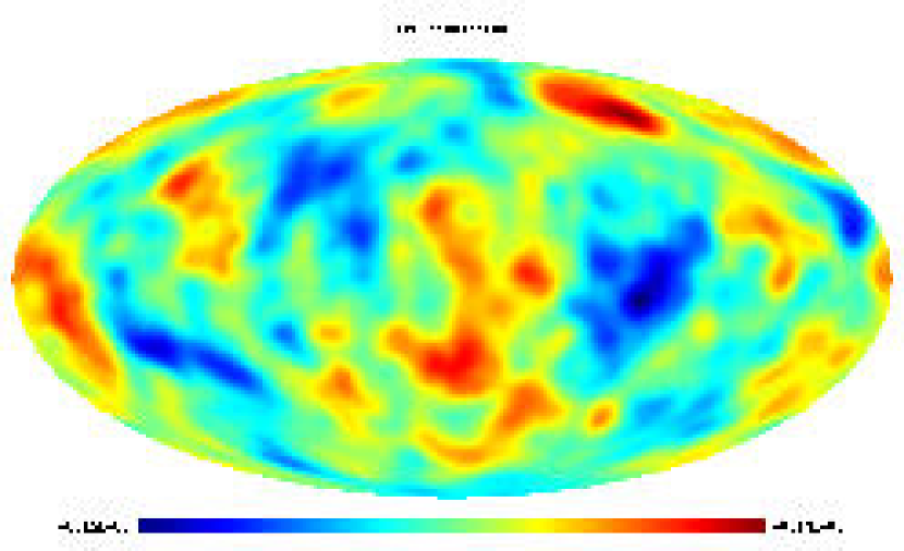
Figure 2: A Gaussian CMB simulation (in units of $K$) smoothed with a Gaussian beam of FWHM=$8^{\circ}$ is shown.

3.1.2 The Laplacian

The Laplacian is the addition of two Gaussian variables with the same dispersion and therefore it also follows a Gaussian distribution with dispersion $\sigma_{2}$.

$$p\left(\lambda_{+}\right)=\frac{1}{\sqrt{2\pi}\sigma_{2}}\exp^{-\frac{1}{2\sigma_{2}^{2}}\left(\lambda_{+}\right)^{2}}~{}.$$ (44)

The Laplacian is defined in the interval $\lambda_{+}\in\left(-\infty,\infty\right)$. As an example, we show the Laplacian of a CMB Gaussian simulation in Fig. 3 (bottom left panel). Note that those regions with low values of $\lambda_{+}$ correspond to regions with high positive curvature in the initial temperature field, and analogously regions with high values of $\lambda_{+}$ correspond to regions with high negative curvature in $T$.

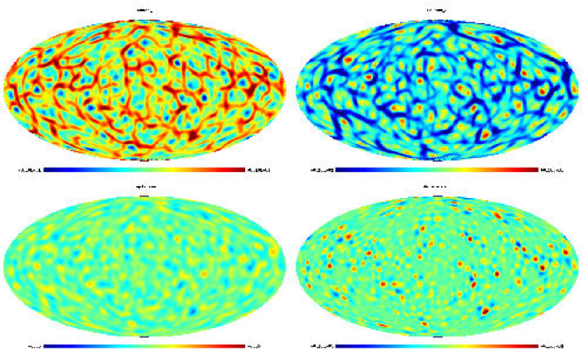
Figure 3: Hessian matrix scalars associated to the temperature map of Fig. 2 are shown: the eigenvalues $\lambda_{1}$ (top left) and $\lambda_{2}$ (top right), the laplacian (bottom left) and the determinant (bottom right).

3.1.3 The determinant of A

Using equation (18), we can construct a semi-analytical expression for the pdf of the determinant:

$$p\left(d\right)=C_{d}e^{wd}\int_{0}^{\infty}e^{ax^{2}}K_{0}\left(\frac{w}{\rho}|x^{2}+d|\right)dx~{},$$ (45)

where $d\in\left(-\infty,\infty\right)$ and the constants are

$$C_{d} = \frac{2}{\pi\sqrt{2\pi\left(1-\rho^{2}\right)}}\frac{1}{\sigma_{r}^{2}\sigma_{t}}~{},$$

$$w = \frac{\rho}{1-\rho^{2}}\frac{1}{\sigma_{r}^{2}}~{},~{}~{}~{}a~{}=~{}w-\frac{1}{2\sigma_{t}^{2}}~{}.$$ (46)

and $K_{0}$ is the zero order modified Bessel function of second kind.

A map of $d$ for the Gaussian CMB simulation shown in Fig. 2, is given in Fig. 3 (bottom right panel). Positive values of $d$ correspond to hill and lake points, so the most curved hills and valleys in the original field are given by the highest values of $d$.

3.2 The distortion scalars

3.2.1 The shear

The shear is the addition of two independent squared Gaussian variables with the same dispersion. Therefore, it follows a $\chi^{2}_{2}$ distribution function with mean and dispersion equal to $<y>=\sigma_{y}=\frac{1}{4}\sigma_{2}^{2}-\frac{1}{2}\sigma_{1}^{2}$.

$$p\left(y\right)=\frac{1}{\sigma_{y}}e^{-\frac{y}{\sigma_{y}}}~{},$$ (47)

where $y\in[0,\infty)$. The map of the shear of a Gaussian CMB simulation is shown in the top left panel of Fig. 4. In the considered example, we find that large values of $y$ are concentrated in regions which usually correspond to saddle points with high values of $\mid\lambda_{i}\mid$ in the original map.

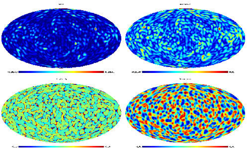
Figure 4: The distortion scalars associated to the temperature map presented in Fig. 2 are plotted. They are the shear (top left), the distortion (top right), the ellipticity (bottom left) and the shape index (bottom right).

3.2.2 The distortion

The distortion is proportional to the square root of the shear, thus its probability density function can be easily obtained from the one of the shear.

$$p(\lambda_{-})=\frac{1}{\sigma_{y}}\frac{\lambda_{-}}{2}e^{-\frac{\lambda_{-}^{2}}{4\sigma_{y}}}$$ (48)

where $\lambda_{-}$ is positive by construction. In the top right panel of Fig. 4 we show the distortion map for the Gaussian CMB simulation of Fig. 2. The physical information contained in the distortion is basically the same as that of the shear. In fact, both maps show quite similar structure.

3.2.3 The ellipticity

Taking into account equation (27), we can obtain the pdf of the ellipticity:

$$p\left(e\right)=2\sigma_{S}\sigma_{R}^{2}\left|e\right|\left[\frac{1}{\sigma_{S}^{2}+4\sigma_{R}^{2}e^{2}}\right]^{\frac{3}{2}}~{},$$ (49)

where $e\in\left(-\infty,\infty\right)$. The map of the ellipticity computed for a Gaussian CMB simulation is given in Fig. 4 (bottom left panel). It is seen that the largest values of $\mid e\mid$ correspond to saddle points surrounding hill or lake points which form compact regions.

3.2.4 The shape index

The shape index pdf can be easily derived from the one of the ellipticity:

$$p\left(\iota\right)=\frac{\sigma_{S}\sigma_{R}^{2}\pi}{4}\frac{\left|\cos{\left(\frac{\pi}{2}\iota\right)}\right|}{\left|\sin^{3}{\left(\frac{\pi}{2}\iota\right)}\right|}\left[\sigma_{S}^{2}+\sigma_{R}^{2}\frac{\cos^{2}{\left(\frac{\pi}{2}\iota\right)}}{\sin^{2}{\left(\frac{\pi}{2}\iota\right)}}\right]^{-\frac{3}{2}}~{}.$$ (50)

Note that the shape index is bound and takes values in the range $\iota\in\left[-1,1\right]$. The structure of the shape index for a Gaussian CMB simulation is shown in the bottom right panel of Fig. 4. This scalar presents a similar structure as the one of the ellipticity. Higher values of $\iota$ correspond to lake points in the original temperature field while lower values of $\iota$ correspond to hill points.

3.3 The gradient related scalars

3.3.1 The square of the gradient modulus

Taking into account equation (29), we see that $g$ is given by the addition of two independent squared Gaussian variables with the same dispersion. Therefore this scalar follows a $\chi^{2}_{2}$ distribution with mean and dispersion equal to $<g>=\sigma_{g}=\sigma_{1}^{2}$

$$p(g)=\frac{1}{\sigma_{g}}e^{-\frac{g}{\sigma_{g}}}~{},$$ (51)

where $g\in[0,\infty)$. As an illustration of the structure of the squared modulus of the gradient, we show the gradient map of the low resolution CMB Gaussian simulation of Fig. 2 in the top panel of Fig. 5. Note that those regions where the temperature field changes rapidly correspond to high values of $g$.

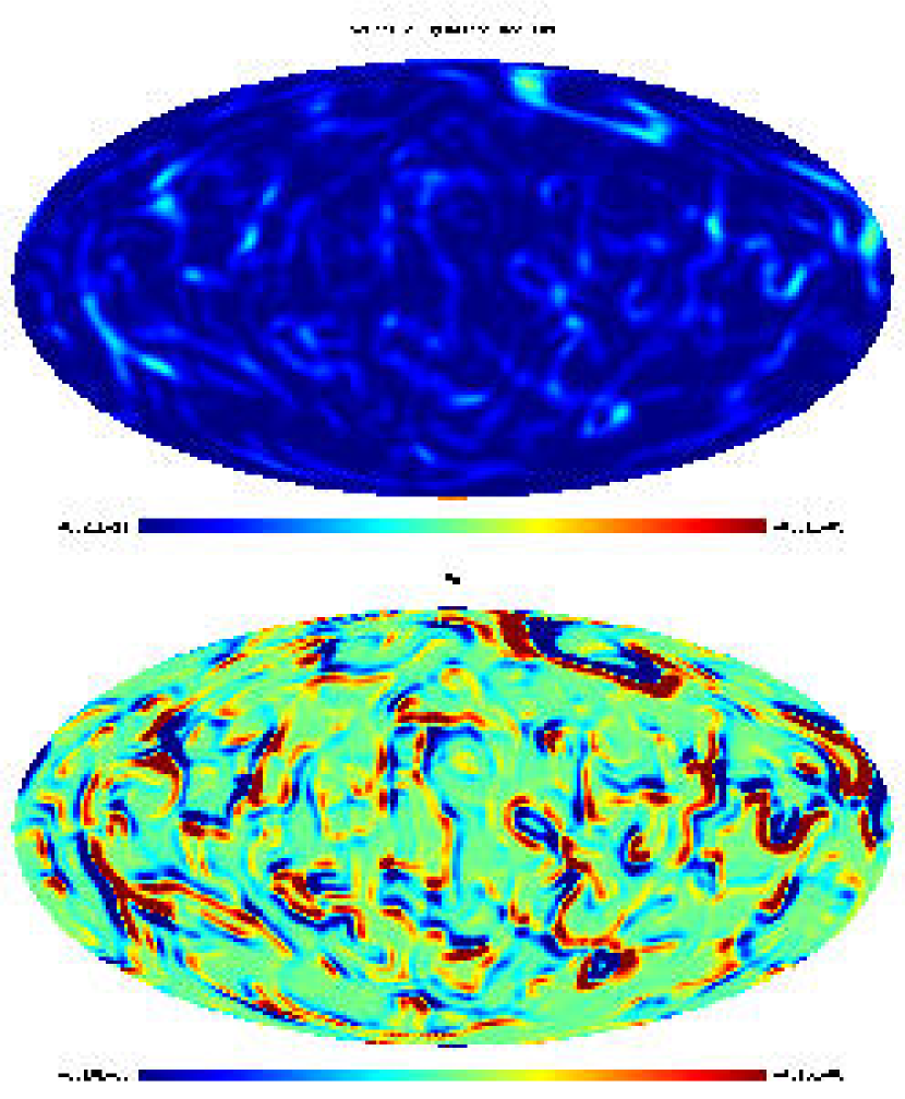
Figure 5: Gradient related scalars associated to the temperature map of Fig. 2 are shown: the squared modulus of the gradient (top), and the gradient derivative (bottom).

3.3.2 Derivative of the square of gradient modulus

$D_{g}$ involves the five Gaussian variables  (5) to  (9) and its probability distribution can be expressed as a function of one integral:

$$p\left(D_{g}\right)=C_{D_{g}}\int_{0}^{\infty}\frac{dz}{z}exp{\left[-\left(\frac{z^{2}}{2\sigma^{2}_{p}}+\frac{D_{g}^{2}}{2\sigma_{r}^{2}z^{4}}\right)\right]}~{},$$ (52)

where $D_{g}\in\left(-\infty,\infty\right)$ and the constant $C_{D_{g}}$ is given by

$$C_{D_{g}}=\frac{1}{\sqrt{2\pi}}\frac{1}{\sigma_{r}\sigma_{p}^{2}}~{}.$$ (53)

The structure of this scalar is shown in the map of Fig. 5 (bottom panel) obtained for a Gaussian CMB simulation. Note that this scalar was defined as the derivative of the squared modulus of the gradient vectorial field, except by a constant factor. In this way it gives us extra information about the directional variation of the gradient, which is not given by $g$.

3.4 The curvature scalars

As shown in equations (34) and (35) the curvature scalars are a function of $1+\mid\vec{\nabla}T\mid^{2}$, which depend on the units of the temperature field and, therefore the shape of the curvature scalars pdf’s will also non-trivially depend on the these units (note that for the previously studied scalars, the units of the field enter just as a normalization factor in the pdf). For this reason we use adimensional fields to calculate the curvatures. In particular, we choose to normalise the initial temperature field to unit dispersion to enhance possible deviations from Gaussianity.

3.4.1 Gaussian curvature

The pdf of the Gaussian curvature can not be obtained in an analytical form but it can be written as a function of two integrals:

$$p\left(\kappa_{G}\right)=C_{\kappa}\int_{0}^{\sqrt{\frac{\rho}{w}}}dv\frac{1}{v^{4}}e^{\rho\frac{\kappa_{G}}{v^{2}}-b\sqrt{\frac{\rho}{w}}\frac{1}{v}}I\left(\frac{\kappa_{G}}{v^{2}}\right)~{},$$ (54)

where $\kappa_{G}\in\left(-\infty,\infty\right)$, and $I\left(\alpha\right)$ is the following integral:

$$I\left(\alpha\right)=\int_{0}^{\infty}dxe^{-\frac{a\rho}{w}x^{2}}K_{0}\left(\left|x^{2}+\alpha\right|\right)~{}.$$ (55)

The constants are given by

$$b = \frac{1}{2\sigma_{p}^{2}}~{},~{}C_{\kappa}~{}=~{}\frac{e^{b}}{\pi\sqrt{2\pi}\sqrt{1-\rho^{2}}}\left(\frac{\rho}{w}\right)^{2}\frac{1}{\sigma_{r}^{2}\sigma_{t}\sigma_{p}^{2}}$$ (56)

$$a = \frac{1}{2\sigma_{t}^{2}}-\gamma~{},~{}w~{}=~{}\frac{\rho}{1-\rho^{2}}\frac{1}{\sigma_{r}^{2}}.$$ (57)

We present in the top panel of Fig. 6 the Gaussian curvature corresponding to the CMB simulation of Fig. 2 (which has been normalised to unit dispersion, as mentioned before). Note that regions with positive values of $\kappa_{G}$ correspond to hill or lake points while negative values correspond to saddle points. This behaviour is similar to the one found for the determinant, but for $\kappa_{G}$ the gradient weights this information in those regions where the later takes large values.

3.4.2 The extrinsic curvature

The extrinsic curvature is defined by equation (35). To obtain an analytical expression for the pdf of this scalar is very complicated and, therefore, we do not include it here.

However, we show in the bottom panel of Fig. 6 the extrinsic curvature map corresponding to the normalised CMB simulation of Fig. 2.

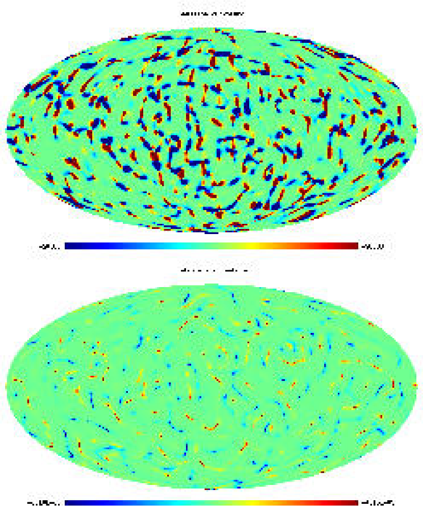
Figure 6: The maps of curvature scalars corresponding to the Gaussian CMB simulation given in Fig. 2 normalised to unity dispersion, (so we work with the adimensional map $\Delta T/\sigma_{0}$.), are shown: Gaussian curvature (top) and extrinsic curvature (bottom)

4 Normalised Scalars

In order to enhance possible non-Gaussian signatures in the temperature field, it would be desirable to study quantities which are independent of the power spectrum of the analysed field. With this aim, we have constructed a new set of scalars that have this property and that are related to the physical scalars of the previous sections. In addition, as will be shown later, these new quantities are mathematically simpler, and allows one to deal in a straightforward manner with anisotropic fields.

In some cases the relation between the normalised and the ordinary scalar, is only a constant factor. In this case the distribution function of these new quantities, can be deduced straightforwardly from the old ones. We can include in this group the square modulus of the gradient and its derivative, the Laplacian, the distortion, the shear and the ellipticity. The rest of the new scalars should be defined using other normalised scalars, and their pdf’s constructed accordingly (see Apendix C).

In the next subsection, we introduce the normalised scalars and give their distribution function for the Gaussian case. We have summarized this information in table  1.

Normalised scalar	Notation	Definition	Domain	pdf
greatest eigenvalue	$\tilde{\lambda}_{1}$	$\frac{1}{2}\left(\tilde{\lambda}_{+}+\tilde{\lambda}_{-}\right)$	$(\tilde{\lambda}_{2},\infty)$	$p(\tilde{\lambda}_{1})=\frac{4}{3\sqrt{2\pi}}e^{-2\tilde{\lambda}_{1}^{2}}\left(1+\sqrt{\frac{2\pi}{3}}\tilde{\lambda}_{1}e^{2\frac{\tilde{\lambda}_{1}^{2}}{3}}\left[1+erf\left(\sqrt{\frac{2}{3}}\tilde{\lambda}_{1}\right)\right]\right)$
lowest eigenvalue	$\tilde{\lambda}_{2}$	$\frac{1}{2}\left(\tilde{\lambda}_{+}-\tilde{\lambda}_{-}\right)$	$(-\infty,\tilde{\lambda}_{1})$	$p(\tilde{\lambda}_{2})=\frac{4}{3\sqrt{2\pi}}e^{-2\tilde{\lambda}_{1}^{2}}\left(1-\sqrt{\frac{2\pi}{3}}\tilde{\lambda}_{1}e^{2\frac{\tilde{\lambda}_{1}^{2}}{3}}\left[1-erf\left(\sqrt{\frac{2}{3}}\tilde{\lambda}_{1}\right)\right]\right)$
Laplacian	$\tilde{\lambda}_{+}$	$-\frac{\lambda_{+}}{\sigma_{2}}$	$(-\infty,\infty)$	$p(\tilde{\lambda}_{+})=\frac{1}{\sqrt{2\pi}}e^{\frac{-\tilde{\lambda}_{+}^{2}}{2}}$
determinant	$\tilde{d}$	$\tilde{\lambda}_{1}\tilde{\lambda}_{2}$	$(-\infty,\infty)$	$p(\tilde{d})=\left\{\begin{array}[]{ll}\frac{4}{\sqrt{3}}e^{4\tilde{d}}&\tilde{d}<0\\ \frac{4}{\sqrt{3}}e^{4\tilde{d}}\left[1-erf\left(\sqrt{6\tilde{d}}\right)\right]&\tilde{d}>0\\ \end{array}\right.$
shear	$\tilde{y}$	$\frac{y}{\sigma_{2}^{2}-2\sigma_{1}^{2}}$	$(0,\infty)$	$p(\tilde{y})=4e^{-4\tilde{y}}$
distortion	$\tilde{\lambda}_{-}$	$\frac{\lambda_{-}}{\sqrt{\sigma_{2}^{2}-2\sigma_{1}^{2}}}$	$(0,\infty)$	$p(\tilde{\lambda}_{-})=2\tilde{\lambda}_{-}e^{-\tilde{\lambda}_{-}^{2}}$
ellipticity	$\tilde{e}$	$\frac{e\sigma_{2}}{\sqrt{\sigma_{2}^{2}-2\sigma_{1}^{2}}}$	$(-\infty,\infty)$	$p(\tilde{e})=4|\tilde{e}|\left(1+8\tilde{e}^{2}\right)^{-\frac{3}{2}}$
shape index	$\tilde{\iota}$	$\frac{2}{\pi}\arctan{\left(-\frac{1}{2\tilde{e}}\right)}$	$(-1,1)$	$p(\tilde{\iota})=\frac{\pi}{2}\frac{|\cos{\left(\frac{\pi}{2}\tilde{\iota}\right)}|}{|\sin^{3}{\left(\frac{\pi}{2}\tilde{\iota}\right)}|}\left[1+2\cot^{2}{\left(\frac{\pi}{2}\tilde{\iota}\right)}\right]^{-\frac{3}{2}}$
gradient	$\tilde{g}$	$\frac{g}{\sigma_{1}^{2}}$	$(0,\infty)$	$p(\tilde{g})=e^{-\tilde{g}}$
derivative of gradient	$\tilde{D}_{g}$	$\frac{D_{g}}{\sqrt{8}\sigma_{r}\sigma_{p}^{2}}$	$(-\infty,\infty)$	$p(\tilde{D}_{g})=\frac{2}{\sqrt{\pi}}\int_{0}^{\infty}{e^{-y^{2}-\frac{\tilde{D}_{g}^{2}}{y^{4}}}\frac{\it{d}y}{y}}$
Gaussian curvature	$\tilde{\kappa}_{G}$	$\frac{\tilde{d}}{\left(1+\tilde{g}\right)^{2}}$	$(-\infty,\infty)$	$p(\tilde{\kappa}_{G})=\left\{\begin{array}[]{ll}-\int_{-\infty}^{\tilde{\kappa}_{G}}\frac{2e}{\tilde{\kappa}_{G}}\sqrt{\frac{z}{3\tilde{\kappa}_{G}}}e^{-\sqrt{\frac{z}{\tilde{\kappa}_{G}}}}e^{4z}dz&\tilde{\kappa}_{G}<0\\ \int_{\tilde{\kappa}_{G}}^{\infty}\frac{2e}{\tilde{\kappa}_{G}}\sqrt{\frac{z}{3\tilde{\kappa}_{G}}}e^{-\sqrt{\frac{z}{\tilde{\kappa}_{G}}}}e^{4z}\left[1-erf\left(\sqrt{6z}\right)\right]dz&\tilde{\kappa}_{G}>0\\ \end{array}\right.$

Table 1: List of the normalised scalars. The pdf’s are valid for any homogeneous and isotropic Gaussian random field, independently of its power spectrum.

In order to test the theoretical distributions obtained for the normalised scalars for the Gaussian case, we have generated 20 full-sky CMB Gaussian simulations, in the way explained in section 3. A map of the studied normalised scalar is then obtained for each simulation and a distribution function of the scalar is constructed. Finally, the average value and dispersion of the distribution function from the 20 simulations is computed and plotted versus the theoretical distribution.

4.1 The normalised Hessian matrix scalars

4.1.1 The normalised eigenvalues

The normalised eigenvalues are defined in terms of the original eigenvalues through the following expression:

$$\left(\begin{array}[]{c}\tilde{\lambda}_{1}\\ \tilde{\lambda}_{2}\end{array}\right)=\frac{1}{2}\left(\begin{array}[]{cc}\frac{1}{\sigma_{2}}+\frac{1}{\sqrt{\sigma_{2}^{2}-2\sigma_{1}^{2}}}&\frac{1}{\sigma_{2}}-\frac{1}{\sqrt{\sigma_{2}^{2}-2\sigma_{1}^{2}}}\\ \frac{1}{\sigma_{2}}-\frac{1}{\sqrt{\sigma_{2}^{2}-2\sigma_{1}^{2}}}&\frac{1}{\sigma_{2}}+\frac{1}{\sqrt{\sigma_{2}^{2}-2\sigma_{1}^{2}}}\end{array}\right)\left(\begin{array}[]{c}\lambda_{1}\\ \lambda_{2}\end{array}\right)$$ (58)

Therefore analogously to the original eigenvalues, $\tilde{\lambda}_{2}<\tilde{\lambda}_{1}<\infty$ and $-\infty<\tilde{\lambda}_{2}<\tilde{\lambda}_{1}$. Note that for a power spectrum as the one of the CMB, we have $\sigma_{1}<<\sigma_{2}$. Using this approximation we find for the previous equation that the normalised eigenvalues are approximately proportional to the original ones and, therefore, have basically the same physical meaning. Their distribution functions for the Gaussian case are given by (see Appendix C):

$$p(\tilde{\lambda}_{1})=\frac{4e^{-2\tilde{\lambda}_{1}^{2}}}{3\sqrt{2\pi}}\left\{1+\sqrt{\frac{2\pi}{3}}\tilde{\lambda}_{1}e^{2\frac{\tilde{\lambda}_{1}^{2}}{3}}\left[1+{\rm erf}\left(\sqrt{\frac{2}{3}}\tilde{\lambda}_{1}\right)\right]\right\}$$ (59)

$$p(\tilde{\lambda}_{2})=\frac{4e^{-2\tilde{\lambda}_{2}^{2}}}{3\sqrt{2\pi}}\left\{1-\sqrt{\frac{2\pi}{3}}\tilde{\lambda}_{2}e^{2\frac{\tilde{\lambda}_{2}^{2}}{3}}\left[1-{\rm erf}\left(\sqrt{\frac{2}{3}}\tilde{\lambda}_{2}\right)\right]\right\}$$ (60)

The pdf for $\tilde{\lambda}_{1}$ and $\tilde{\lambda}_{2}$, together with the corresponding results obtained from the simulations, are shown in the top panels of Fig. 7.

Figure 7: Theoretical distributions and results obtained from CMB Gaussian simulations for the normalised eigenvalues (top left and right), the normalised Laplacian (bottom left) and the normalised determinant (bottom right). The normalised Laplacian is Gaussian distributed whereas the other three normalised scalars follow different non-Gaussian distribution.

4.1.2 The normalised Laplacian

The normalised Laplacian, $\tilde{\lambda}_{+}$, is defined using the original Laplacian:

$$\tilde{\lambda}_{+}=-\frac{\lambda_{+}}{\sigma_{2}}$$ (61)

where, by definition $-\infty<\tilde{\lambda}_{+}<\infty$. The normalised Laplacian of a HIGRF follows a Gaussian distribution with zero mean and unit dispersion:

$$p(\tilde{\lambda}_{+})=\frac{1}{\sqrt{2\pi}}e^{\frac{-\tilde{\lambda}_{+}^{2}}{2}}.$$ (62)

Fig. 7 (bottom left panel) shows that the distribution obtained for $\tilde{\lambda}_{+}$ from the Gaussian CMB simulations perfectly follows its theoretical pdf.

4.1.3 The normalised determinant

The normalised determinant, $\tilde{d}$, is defined analogously to the original one, using the normalised scalars $\tilde{\lambda}_{1}$ and $\tilde{\lambda}_{2}$ as follows:

$$\tilde{d}=\tilde{\lambda}_{1}\tilde{\lambda}_{2}$$ (63)

where $\tilde{d}\in(-\infty,\infty)$. Using the approximation $\sigma_{1}<<\sigma_{2}$ valid for CMB maps, the normalised determinant becomes proportional to the original determinant.

The probability density function of the normalised determinant for the Gaussian case is (See Appendix  C).

$$p(\tilde{d})=\left\{\begin{array}[]{ll}\frac{4}{\sqrt{3}}e^{4\tilde{d}}&\tilde{d}<0\\ \frac{4}{\sqrt{3}}e^{4\tilde{d}}\left[1-erf\left(\sqrt{6\tilde{d}}\right)\right]&\tilde{d}>0\\ \end{array}\right.$$ (64)

The bottom right panel of Fig. 7 shows that the agreement between the theoretical pdf and that obtained from simulated CMB maps is very good.

4.2 The normalised distortion scalars

4.2.1 The normalised shear

The normalised shear, $\tilde{y}$, is defined as a constant factor times the original shear,

$$\tilde{y}=\frac{y}{\sigma_{2}^{2}-2\sigma_{1}^{2}}$$ (65)

so inherited by the original shear, $0<\tilde{y}<\infty$. The distribution function of this normalised quantity for the Gaussian case is simpler than for $y$ :

$$p(\tilde{y})=4e^{-4\tilde{y}}.$$ (66)

The comparison between this probability density function and the one obtained from 20 Gaussian CMB simulations, is shown in the top left panel of Fig. 8. Note that the agreement between the theoretical curve and the results obtained from simulations is very good.

Figure 8: Theoretical distributions compared to the results from CMB Gaussian simulations for the normalised shear (top left), the normalised distortion (top right), the normalised ellipticity (bottom left) and the normalised shape index (bottom right).

4.2.2 The normalised distortion

The normalised distortion, $\tilde{\lambda}_{-}$, is defined by:

$$\tilde{\lambda}_{-}=\frac{\lambda_{-}}{\sqrt{\sigma_{2}^{2}-2\sigma_{1}^{2}}}$$ (67)

and analogously to the original distortion, $0<\tilde{\lambda}_{-}<\infty$. The probability density function of the normalised distortion for a HIGRF is

$$p(\tilde{\lambda}_{-})=2\tilde{\lambda}_{-}e^{-\tilde{\lambda}_{-}^{2}}.$$ (68)

This theoretical distribution versus the one obtained from simulations are given in the top right panel of Fig.8.

4.2.3 The normalised ellipticity

The normalised ellipticity, $\tilde{e}$, is proportional to $e$ :

$$\tilde{e}=\frac{\sigma_{2}}{\sqrt{\sigma_{2}^{2}-2\sigma_{1}^{2}}}e$$ (69)

where, by construction $-\infty<\tilde{e}<\infty$. The probability density function of the normalised ellipticity of a HIGRF is

$$p(\tilde{e})=4|\tilde{e}|\left(1+8\tilde{e}^{2}\right)^{-\frac{3}{2}}.$$ (70)

Note that this distribution function has very long tails and that $<\tilde{e}^{2}>$ is not defined. This problem was inherited from the original ellipticity pdf, and motivates the introduction of the shape index, which is a bounded quantity.

The theoretical pdf and the results obtained from CMB simulations are compared in the bottom left panel of Fig. 8.

4.2.4 The normalised shape index

The normalised shape index, $\tilde{\iota}$, is defined in terms of the normalised ellipticity in an analogous way to the definition of the original shape index, (see equation (28)):

$$\tilde{\iota}=\frac{2}{\pi}\arctan{\left(-\frac{1}{2\tilde{e}}\right)}$$ (71)

Therefore $-1<\tilde{\iota}<1$. The distribution function of the normalised shape index, for the Gaussian case, is deduced from the one of the normalised ellipticity through simple transformations:

$$p(\tilde{\iota})=\frac{\pi}{2}\frac{|\cos{\left(\frac{\pi}{2}\tilde{\iota}\right)}|}{|\sin^{3}{\left(\frac{\pi}{2}\tilde{\iota}\right)}|}\left[1+2\cot^{2}{\left(\frac{\pi}{2}\tilde{\iota}\right)}\right]^{-\frac{3}{2}}.$$ (72)

The bottom right panel of Fig. 8 shows the good agreement between the theoretical prediction and the results obtained from simulations for the normalised shape index.

4.3 The normalised gradient related scalars

4.3.1 The normalised square of the gradient modulus

The normalised square of the gradient modulus, $\tilde{g}$, is defined as the original gradient times a constant factor:

$$\tilde{g}=\frac{g}{\sigma_{1}^{2}},$$ (73)

therefore $0<\tilde{g}<\infty$ and the resulting distribution function of this normalised quantity for the Gaussian case, is simply

$$p(\tilde{g})=e^{-\tilde{g}}.$$ (74)

The top panel of Fig. 9 shows the theoretical distribution function compared to the results obtained from simulations for $\tilde{g}$, showing excellent agreement.

Figure 9: Comparison between the theoretical pdf and the one obtained from Gaussian CMB simulations for the normalised square of the gradient modulus (top) and the normalised derivative of the gradient.

4.3.2 The normalised derivative of the square of gradient modulus

The normalised derivative of the square of the gradient modulus, $\tilde{D_{g}}$, is proportional to the original scalar:

$$\tilde{D}_{g}=\frac{D_{g}}{\sqrt{8}\sigma_{r}\sigma_{p}^{2}},$$ (75)

so inherited by the original scalar, $-\infty<\tilde{D}_{g}<\infty$. The probability density function of this normalised scalar for the Gaussian case, is trivially obtained from the pdf of the primitive scalar:

$$p(\tilde{D}_{g})=\frac{2}{\sqrt{\pi}}\int_{0}^{\infty}{e^{-y^{2}-\frac{\tilde{D}_{g}^{2}}{y^{4}}}\frac{\it{d}y}{y}}.$$ (76)

The bottom panel of Fig. 9 shows the theoretical pdf and the one obtained from simulations for $\tilde{D}_{g}$. Again the agreement is very good.

4.4 The normalised curvature scalars

4.4.1 The normalised Gaussian curvature

The normalised Gaussian curvature, $\tilde{\kappa}_{G}$, is defined in terms of the normalised determinant and the normalised gradient, as follows:

$$\tilde{\kappa}_{G}=\frac{\tilde{d}}{\left(1+\tilde{g}\right)^{2}},$$ (77)

where by construction $-\infty<\tilde{\kappa}_{G}<\infty$. The pdf of the normalised Gaussian curvature of a HIGRF is given by:

$$p(\tilde{\kappa}_{G})=\left\{\begin{array}[]{ll}-\int_{-\infty}^{\tilde{\kappa}_{G}}\frac{2e^{4z+1}}{\tilde{\kappa}_{G}}\sqrt{\frac{z}{3\tilde{\kappa}_{G}}}e^{-\sqrt{\frac{z}{\tilde{\kappa}_{G}}}}dz&\tilde{\kappa}_{G}<0\\ \int_{\tilde{\kappa}_{G}}^{\infty}\frac{2e^{4z+1}}{\tilde{\kappa}_{G}}\sqrt{\frac{z}{3\tilde{\kappa}_{G}}}e^{-\sqrt{\frac{z}{\tilde{\kappa}_{G}}}}\\ ~{}~{}\left[1-erf\left(\sqrt{6z}\right)\right]dz&\tilde{\kappa}_{G}>0\\ \end{array}\right.$$ (78)

The comparison between the theoretical and simulated results are shown in the top panel of Fig. 10.

Figure 10: Comparison between the theoretical pdf and the one obtained from 20 Gaussian CMB simulations for the normalised Gaussian curvature (top), and distribution function obtained from simulations for the normalised extrinsic curvature (bottom).

4.4.2 The normalised extrinsic curvature

The normalised extrinsic curvature, $\tilde{\kappa}_{ex}$, is defined analogously to the original scalar, using equation (35):

$$\tilde{\kappa}_{ex}=\frac{1}{2}~{}\frac{1}{\sqrt{1+\tilde{g}}}\left[\tilde{\lambda}_{+}-\frac{\tilde{D}_{g}}{\left(1+\tilde{g}\right)}\right]~{},$$ (79)

Therefore $-\infty<\tilde{\kappa}_{ex}<\infty$. As for the original ${\kappa}_{ex}$, it is very complicated to obtain an analytical expression for the pdf of this normalised scalar. However we have included in the bottom panel of Fig 10, the pdf of the normalised extrinsic curvature obtained from 20 Gaussian CMB simulations.

4.5 Correlations between normalised scalars

By looking at the definitions of the different scalars, it becomes apparent that some of the scalars are related to each other. In order to know how much independent information they contain, it is interesting to study the correlations between the different scalars. Using simulations, we have calculated these correlations for a HIGRF which are given in table 2. We have included all the normalised scalars except for the ellipticity, due to the fact that the dispersion of this quantity is not defined and, therefore, the usual correlation coefficient can not be calculated. However, the ellipticity and the shape index are very closely related and thus it is expected that the correlations between the ellipticity and the rest of the scalars will be similar to those obtained for the shape index.

It is interesting to note that the gradient of the modulus, $\tilde{g}$, is the only scalar which is uncorrelated with all the considered scalars. On the contrary, the eigenvalues, $\tilde{\lambda}_{1}$ and $\tilde{\lambda}_{2}$, have some degree of correlation (or anticorrelation) with all the scalars (except for $\tilde{g}$). Within the Hessian scalars, we see that only the normalised Laplacian, $\tilde{\lambda}_{+}$, and determinant, $\tilde{d}$, are uncorrelated between them. $\tilde{\lambda}_{+}$ is also uncorrelated with two of the normalised distortion scalars (the shear, $\tilde{y}$, and the distorsion, $\tilde{\lambda}_{-}$) as well as with Gaussian curvature $\tilde{\kappa}_{g}$. Conversely, $\tilde{d}$ has some correlation with these three scalars but is uncorrelated with the normalised shape index, $\tilde{\iota}$, the derivative of the gradient, $\tilde{D}_{g}$ and extrinsic curvature, $\tilde{\kappa}_{ex}$. With regard to the distortion scalars, $\tilde{y}$ and $\tilde{\lambda}_{-}$ are strongly correlated, which is expected since $\tilde{y}$ is, except by a constant factor, the square of $\tilde{\lambda}_{-}$. However, these two scalars are uncorrelated with the shape index $\tilde{\iota}$. It is also interesting to note that $\tilde{\kappa}_{G}$ is uncorrelated with $\tilde{\kappa}_{ex}$.

	$\tilde{\lambda}_{1}$	$\tilde{\lambda}_{2}$	$\tilde{\lambda}_{+}$	$\tilde{d}$	$\tilde{y}$	$\tilde{\lambda}_{-}$	$\tilde{\iota}$	$\tilde{g}$	$\tilde{D}_{g}$	$\tilde{\kappa}_{G}$	$\tilde{\kappa}_{ex}$
$\tilde{\lambda}_{1}$	1.00	0.64	0.91	-0.23	0.40	0.42	-0.83	0	-0.52	-0.19	0.89
$\tilde{\lambda}_{2}$	0.64	1.00	0.91	0.23	-0.40	-0.42	-0.83	0	-0.52	0.19	0.89
$\tilde{\lambda}_{+}$	0.91	0.91	1.00	0	0	0	-0.92	0	-0.58	0	0.99
$\tilde{d}$	-0.23	0.23	0	1.00	-0.58	-0.55	0	0	0	0.83	0
$\tilde{y}$	0.40	-0.40	0	-0.58	1.00	0.96	0	0	0	-0.48	0
$\tilde{\lambda}_{-}$	0.42	-0.42	0	-0.55	0.96	1.00	0	0	0	-0.46	0
$\tilde{\iota}$	-0.83	-0.83	-0.92	0	0	0	1.00	0	0.53	0	-0.91
$\tilde{g}$	0	0	0	0	0	0	0	1.00	0	0	0
$\tilde{D}_{g}$	-0.52	-0.52	-0.58	0	0	0	0.53	0	1.00	0	-0.57
$\tilde{\kappa}_{G}$	-0.19	0.19	0	0.83	-0.48	-0.46	0	0	0	1.00	0
$\tilde{\kappa}_{ex}$	0.89	0.89	0.99	0	0	0	-0.91	0	-0.57	0	1.00

Table 2: Correlations between the normalised scalars.

5 Treatment of instrumental noise and masks

Real data contain not only the cosmological signal but also contaminating emissions and instrumental noise. The Galactic region, where the Galactic foregrounds dominate, is usually masked from the data. It is also a common procedure to mask the emission coming from extragalactic point sources. These masked pixels are then discarded from the analysis.

In addition, the instrumental noise produces discontinuities from pixel to pixel in the map, since this noise is assumed to be, in general, uncorrelated (white noise). The discontinuities introduce problems in the calculation of the derivatives. In order to deal with this issue, we will smooth the CMB signal plus noise with a Gaussian beam of FWHM equal to 2.4 times the pixel size (where we assume that this is the size of the Gaussian beam used to filter the original CMB signal).

Assuming that the white noise is homogeneous and isotropic, its power spectrum is given by:

$$C_{\ell}^{n}=\frac{4\pi\sigma_{n}^{2}}{N_{pixtot}}$$ (80)

where $\sigma_{n}$ is the noise dispersion and $N_{pixtot}$ is the total number of pixels. So the resulting power spectrum of the noisy simulations can be expressed as follows:

$$C_{\ell}=[C_{\ell}^{s}e^{-\ell\left(\ell+1\right)\sigma_{g}^{2}}+C_{\ell}^{n}]e^{-\ell\left(\ell+1\right)\sigma_{g}^{2}}$$ (81)

where $\sigma_{g}$ is the Gaussian beam dispersion and $C_{\ell}^{s}$ is the CMB power spectrum.

However, in most experiments, the instrumental noise is usually an anisotropic Gaussian random field, charactarised by a different dispersion at each pixel $\sigma_{n}(\vec{x})$ (with $\vec{x}$ the unitary vector on the sphere in the direction of observation). In order to deal with anisotropic noise, we have built a “pixel-dependent power spectrum” $H_{\ell}(\vec{x})$ in the following way:

$$H_{\ell}(\vec{x})=\left[C_{\ell}^{s}e^{-\ell\left(\ell+1\right)\sigma_{g}^{2}}+\frac{4\pi\sigma_{n}^{2}(\vec{x})}{N_{pixtot}}\right]e^{-\ell\left(\ell+1\right)\sigma_{g}^{2}}.$$ (82)

$H_{\ell}(\vec{x})$ would be the power spectrum of a map that contain the filtered CMB plus isotropic noise with dispersion $\sigma_{n}(\vec{x})$, and filtered again with a Gaussian beam of disperson $\sigma_{g}$. In practice, due to this second smoothing, the dispersion of the noise in a given pixel would depend not only on the noise level on that position but also of its neighbours. However, provided that the dispersion of the noise varies smoothly, which is usually the case, the previous equation is a good approximation to the “power spectrum in each pixel”.

Since, by construction, the normalised scalars are independent of the power spectrum of the field, we can obtain these quantities for each pixel, taking into account equation (82). We just need to construct the moment fields on the sphere $\sigma_{0}(\vec{x}),\sigma_{1}(\vec{x})$ and $\sigma_{2}(\vec{x})$ using equation (36), where the $C_{\ell}$’s are now given by $H_{\ell}(\vec{x})$. The normalised scalars are then calculated by introducing these pixel-dependent moments on their corresponding definitions. The probability distribution function obtained from the map of the normalised scalar constructed in this way will follow the corresponding theoretical distribution given in the previous section. This is one of the advantages of working with the normalised scalars. Note that if we construct the ordinary scalars for a map containing anisotropic noise, the resulting probability distribution will not longer follow the theoretical pdf for a Gaussian field.

In addition to noise we also have a masked region, which introduces discontinuities in the boundary of the mask. Moreover, we have no information about the field inside these masked regions. As before, in order to deal with this problem, the first step is to smooth the masked map (with the pixels of the mask set to zero) with a Gaussian beam of FWHM equal to 2.4 times the pixel size. As already mentioned, this solves the problem of the discontinuities of the noise and also reduces the mask boundary problem. However a more sophisticated procedure is necessary to eliminate the effect of the mask, since if we calculate the normalised scalars from this smoothed masked map, those pixels close to the boundary would be strongly contaminated by the spurious signal of the mask. Nevertheless, the values of the normalised scalars in those pixels far enough from the mask would be correct. Therefore we need to generate an extended mask that eliminates from the analysis not only the original masked pixels but also those pixels in the neighborhood of the mask. The particular shape of this extended mask would depend on the original mask but also on the particular normalised scalar that we are considering.

We can obtain the extended mask for each normalised scalars using simulations. In particular, we construct and compare one $\it{exact}$ and one $\it{approximated}$ map for the considered quantity for each simulated map. The exact map $I_{e}$ is constructed, simply, by calculating the normalised scalar from the smoothed noisy map; since the derivatives are obtained without masking any region, they will be properly calculated. The approximated map $I_{a}$ is obtained by calculating the corresponding normalised scalar from the masked smoothed noisy map. In this case the derivatives of those pixels close to the boundary of the masked region would be heavily contaminated by the mask. For each simulation, at each pixel outside the original mask, we calculate then the error quantity $\epsilon$ defined as:

$$\epsilon=\frac{|I_{e}-I_{a}|}{\sigma_{e}}$$ (83)

where $\sigma_{e}$ is the dispersion of the exact map for the corresponding simulation. The average of this quantity over a large number of simulations is then obtained and we have a map of $\epsilon$ at each pixel outside the original mask. The extended mask will be formed, in addition to the pixels of the original mask, by those pixels with $\epsilon$ greater than a fixed value $\epsilon_{*}$, that is, we keep for the analysis only those pixels where the value of the considered normalised scalar is reasonably close to the correct value and therefore are not appreciably contaminated by the presence of the mask. Considering only the pixels outside the extended mask, the distribution of the normalised scalars should follow the theoretical pdf’s found in previous sections.

In order to test the method using realistic simulations, we have studied the normalised scalars using masked CMB maps containing anisotropic noise. We have used the Kp0 mask, defined in Bennett et al. 2003b, which covers approximately a 24 per cent of the sky. The anisotropic noise has been simulated with a level equal to that expected for the noise-weighted average of the Q, V and W WMAP channels (Komatsu et al. 2003) after two years of observation. The signal-to-noise ratio per pixel of the simulations ranges from 1.6 to 5.9 (at resolution $N_{side}=256$). To obtain the extended mask we have used 100 simulations and find that a value of $\epsilon_{*}=0.1$ provides good results. We have then obtained from the simulations the pdf for each of the normalised scalars (but using only those pixels outside the extended mask) and compare it with the theoretical pdf. Table 3 gives the percentage of useful pixels that are kept after applying the corresponding extended mask for the normalised scalars.

Scalar	Useful pixels (%)
$\tilde{\lambda}_{1}$	70.6
$\tilde{\lambda}_{2}$	70.5
$\tilde{\lambda}_{+}$	70.1
$\tilde{d}$	72.0
$\tilde{y}$	67.8
$\tilde{\lambda}_{-}$	69.2
$\tilde{\iota}$	68.1
$\tilde{g}$	70.7
$\tilde{D}_{g}$	71.8
$\tilde{\kappa}_{G}$	70.7
$\tilde{\kappa}_{ex}$	70.1

Table 3: The percentage of useful pixels kept after applying the extended masks obtained with $\epsilon_{*}=0.1$ for the normalised scalars.

For all the normalised scalars we see that approximately a 70 per cent of the pixels can be used for the analysis, loosing only around a 6 per cent of the sky with respect to the Kp0 mask. The extended mask for the normalised ellipticity can not be obtained using the error quantity $\epsilon$, since the dispersion of this scalar is not defined. Alternative error quantities could be used to obtain its extended mask. However, for simplicity, we have used the mask obtained for the normalised shape index, since these two quantities are closely related.

The pdf’s obtained from 100 simulations (using only those pixels outside the extended mask) for the normalised Laplacian, distortion and shape index are compared to their corresponding theoretical pdf’s showing an excellent agreement. Similar results are obtained for the rest of normalised scalars (including the ellipticity), using their corresponding extended masks (which are not shown for the sake of brevity).

Figure 11: The distribution obtained from 100 simulations compared to the corresponding theoretical pdf is shown for three different normalised scalars: Laplacian (top), distortion (middle) and shape index (bottom). The distributions have been obtained using only those pixels outside the extended mask (with $\epsilon_{*}$=0.10).

6 Conclusions

In this paper we have introduced several scalar quantities on the sphere and we have shown how to calculate them for a CMB map directly from the $a_{\ell m}$ harmonic coefficients. In particular, we have considered the square modulus of the gradient, the Laplacian, the determinant of the negative Hessian matrix, the distorsion, the shear, the ellipticity, the shape index, the eigenvalues of the negative Hessian matrix, the Gaussian curvature, the extrinsic curvature and the gradient derivative. Assuming a homogeneous and isotropic Gaussian field, we have derived analytical or semi-analytical expressions for the pdf’s of each of the scalars. For convenience, we define normalised scalars which have more simple distribution functions than ordinary scalars. Therefore, for these normalised scalars we have tested the theoretical results with simulations, showing an excellent agreement.

We propose these scalars to study the Gaussian character of the CMB. In particular, we aim to test their power using non-Gaussian CMB simulations based in the Edgeworth expansion (Martínez-González et al. 2002). Moreover, we plan to apply this method in future works to both physically motivated non-Gaussian models and the WMAP data. Finally, we would like to point out that the study of the scalars can be adapted, for instance, to deal with regions or extrema above (or below) different thresholds. This will also be studied in a future work.

Appendix A Derivatives on the sphere

In this appendix we derive the harmonic coefficients of the first and second derivatives of the temperature field as a function of the $a_{\ell m}$. With these expressions and using the HEALPix package it is straightforward to calculate the maps of the field derivatives as well as the scalars.

It is a common procedure to write the temperature field on the sphere as a series of harmonic functions:

$$T(\theta,\phi)=\sum_{\ell,m}a_{\ell m}Y_{\ell m}(\theta,\phi)~{}.$$ (84)

The spherical harmonic functions constitute an orthonormal complete set. Also, they are eigenvectors of the momentum operators $L_{z}$ and $L^{2}$:

$$L_{z}Y_{\ell m} = mY_{\ell m}~{},$$ (85)

$$L^{2}Y_{\ell m} = \ell(\ell+1)Y_{\ell m}~{}.$$ (86)

In addition, the $L_{+}$ and $L_{-}$ operators that are defined:

$$L_{\pm}=L_{x}\pm iL_{y}~{},$$ (87)

act on the spherical harmonic functions in the following way:

$$L_{\pm}Y_{\ell m}=\sqrt{\left(\ell\pm m+1\right)\left(\ell\mp m\right)}Y_{\ell m\pm 1}~{}.$$ (88)

In order to obtain the derivatives of the field, we will write them as a function of the previous operators:

$$\frac{\partial}{\partial\theta} = \frac{1}{2}\left[e^{-i\phi}L_{+}-e^{i\phi}L_{-}\right]~{},$$ (89)

$$\frac{\partial}{\partial\phi} = iL_{z}~{}.$$ (90)

On the other hand, we will also make use of the following common spherical harmonic relations:

$$e^{-i\phi}\sin{\theta}~{}Y_{\ell m+1} = \sqrt{\frac{\left(\ell-m\right)\left(\ell-m+1\right)}{\left(2\ell+1\right)\left(2\ell+3\right)}}Y_{\ell+1m}-$$ (91)

$$- \sqrt{\frac{\left(\ell+m\right)\left(\ell+m+1\right)}{\left(2\ell-1\right)\left(2\ell+1\right)}}Y_{\ell-1m}~{},$$

$$e^{i\phi}\sin{\theta}~{}Y_{\ell m-1} = \sqrt{\frac{\left(\ell+m\right)\left(\ell+m+1\right)}{\left(2\ell+1\right)\left(2\ell+3\right)}}Y_{\ell+1m}-$$ (92)

$$- \sqrt{\frac{\left(\ell-m\right)\left(\ell-m+1\right)}{\left(2\ell-1\right)\left(2\ell+1\right)}}Y_{\ell-1m}~{},$$

$$\cos{\theta}~{}Y_{\ell m} = \sqrt{\frac{\left(\ell-m+1\right)\left(\ell+m+1\right)}{\left(2\ell+1\right)\left(2\ell+3\right)}}Y_{\ell+1m}+$$ (93)

$$+ \sqrt{\frac{\left(\ell+m\right)\left(\ell-m\right)}{\left(2\ell+1\right)\left(2\ell-1\right)}}Y_{\ell-1m}~{}.$$

Applying the derivative operators given in (89) and (90) to the temperature field (84), and taking into account the previous spherical harmonic relations, it is straightforward to obtain the harmonic coefficients of the fields $\frac{\partial T}{\partial\phi}$ and $\sin\theta\frac{\partial T}{\partial\theta}$, $b_{\ell m}$ and $c_{\ell m}$ respectively, as a function of the harmonic coefficients $a_{\ell m}$ of the original field

$$c_{\ell m}=im~{}a_{\ell m}~{},$$ (94)

$$b_{\ell m}=H_{+}\left(\ell,m\right)a_{\ell+1,m}+H_{-}\left(\ell,m\right)a_{\ell-1,m}~{},$$ (95)

where $H_{\pm}$ are functions of $\ell,m$ given by

$$H_{+}\left(\ell,m\right)=-\left(\ell+2\right)\sqrt{\frac{\left(\ell+m+1\right)\left(\ell-m+1\right)}{\left(2\ell+1\right)\left(2\ell+3\right)}}~{},$$ (96)

$$H_{-}\left(\ell,m\right)=\left(\ell-1\right)\sqrt{\frac{\left(\ell+m\right)\left(\ell-m\right)}{\left(2\ell+1\right)\left(2\ell-1\right)}}~{},$$ (97)

Note that these functions are even on $m$ and that $H_{-}(\ell,\ell)$ is zero for all the $\ell$ values.

Analogously, we can obtain the harmonic coefficients $d_{\ell m}$, $e_{\ell m}$, and $f_{\ell m}$ corresponding to the fields $\frac{\partial^{2}T}{\partial\phi^{2}}$, $\sin^{2}{\theta}\frac{\partial^{2}T}{\partial\theta^{2}}$ and $\sin{\theta}\frac{\partial^{2}T}{\partial\theta\partial\phi}$:

$$d_{\ell m} = -m^{2}a_{\ell m}~{},$$ (98)

$$e_{\ell m} = \left[\left(\frac{\ell\left(\ell+3\right)}{\left(\ell+2\right)^{2}}\right)H_{+}^{2}\left(\ell,m\right)\right.$$ (99)

$$- \left.\left(\frac{\left(\ell+1\right)\left(\ell-2\right)}{\left(\ell-1\right)^{2}}\right)H_{-}^{2}\left(\ell,m\right)\right]a_{\ell m}+$$

$$+ \left[\left(\frac{\ell+3}{\ell+2}\right)H_{+}\left(\ell,m\right)H_{+}\left(\ell+1,m\right)\right]a_{\ell+2,m}+$$

$$+ \left[\left(\frac{\ell-2}{\ell-1}\right)H_{-}\left(\ell,m\right)H_{-}\left(\ell-1,m\right)\right]a_{\ell-2,m}~{},$$

$$f_{\ell m} = im\left[H_{+}\left(\ell,m\right)a_{\ell+1,m}+H_{-}\left(\ell,m\right)a_{\ell-1,m}\right]~{}.$$ (100)

Making use of the previous results and taking into account the different expressions presented along this work, it is straightforward to obtain the maps of the considered scalars.

Appendix B Some useful results regarding spherical harmonic series

In this appendix we present some useful results for spherical harmonic series, which are necessary to calculate the covariances of the variables defined in equations (5-9).

In particular, we have made use of the following expressions which involve the harmonic functions and their derivatives with respect to $\theta$:

$$\sum_{m=-\ell}^{\ell}\frac{\partial Y_{\ell m}}{\partial\theta}Y_{\ell m}^{*}=0~{},$$ (101)

$$\sum_{m=-\ell}^{\ell}\frac{\partial Y_{\ell m}}{\partial\theta}\frac{\partial Y_{\ell m}^{*}}{\partial\theta}=-\sum_{m=-\ell}^{\ell}\frac{\partial^{2}Y_{\ell m}}{\partial\theta^{2}}Y_{\ell m}^{*}=\frac{2l+1}{4\pi}\frac{l(l+1)}{2}~{},$$ (102)

$$\sum_{m=-\ell}^{\ell}\frac{\partial Y_{\ell m}}{\partial\theta}\frac{\partial^{2}Y_{\ell m}^{*}}{\partial\theta^{2}}=0~{}.$$ (103)

Another interesting set of series involve the presence of powers of $m$. In particular, we need:

$$\sum_{m=-\ell}^{\ell}m^{4}Y_{\ell m}^{2}=\frac{2\ell+1}{4\pi}\left[\frac{3}{8}\left[\ell\left(\ell+1\right)\right]^{2}-\frac{1}{2}\ell\left(\ell+1\right)\left[\frac{\cos{2\theta}}{\sin^{2}{\theta}}\right]\right]~{},$$ (104)

$$\sum_{m=-\ell}^{\ell}m^{2}Y_{\ell m}^{2}(\theta,\phi)=\frac{2\ell+1}{4\pi}\frac{l(l+1)}{2}\sin^{2}{\theta}~{},$$ (105)

and applying $\frac{\partial}{\partial\theta}$ to the previous expression, we get:

$$\sum_{m=-\ell}^{\ell}m^{2}\frac{\partial Y_{\ell m}}{\partial\theta}Y_{\ell m}^{*}=\frac{2l+1}{4\pi}\frac{l(l+1)}{2}\sin{\theta}\cos{\theta}~{}.$$ (106)

It can also be be shown that other series that appear in the calculation of the covariances of the variables (5-9) and that involve odd powers of $m$ are zero, such as:

$$\sum_{m=-\ell}^{\ell}m^{i}Y_{\ell m}^{2}=0~{},$$ (107)

$$\sum_{m=-\ell}^{\ell}m^{i}Y_{\ell m}\frac{\partial Y_{\ell m}^{*}}{\partial\theta}=0~{},$$ (108)

$$\sum_{m=-\ell}^{\ell}m^{i}\left[\frac{\partial Y_{\ell m}}{\partial\theta}\right]^{2}=0~{},$$ (109)

$$\sum_{m=-\ell}^{\ell}m^{i}Y_{\ell m}\frac{\partial^{2}Y_{\ell m}^{*}}{\partial\theta^{2}}=0~{},$$ (110)

where $i$ is an odd integer.

Appendix C Normalised scalars distribution functions

In this appendix we give some guidelines on how to deduce the pdf of ordinary scalars for a HIGRF. We also show how to obtain the probability density function of the normalised scalars from that of the original scalars. As an illustration, we focus on the normalised ellipticity and determinant, but similar calculations are needed to obtain the pdf’s of the rest of the scalars.

As explained in section  2, ordinary scalars can be constructed in terms of the Gaussian variables $\{p,q,r,s,t\}$ given in equations (5) to (9). In particular, the ellipticity can be rewritten as:

$$e=-\frac{\sqrt{(r-s)^{2}+(2t)^{2}}}{2(r+s)}~{}.$$ (111)

Let us define the uncorrelated Gaussian variables $R=r+s$, $S=r-s$ and $T=2t$. It is straightforward to show that $\sigma_{R}^{2}=\sigma_{2}^{2}$ and $\sigma_{S}^{2}=\sigma_{T}^{2}=\frac{1}{2}\sigma_{2}^{2}-\sigma_{1}^{2}$. In terms of these new variables, the ellipticity is given by

$$e=-\frac{\sqrt{S^{2}+T^{2}}}{2R}~{}.$$ (112)

Since S, T and R are independent variables, the numerator and the denominator are also independent.

The numerator is the square root of the addition of the square of two Gaussian uncorrelated variables with the same dispersion $\sigma_{S}$. Therefore the numerator, $z$, should follow a Rayleigh distribution:

$$p(z)=\frac{1}{\sigma^{2}_{S}}ye^{-\frac{z^{2}}{2\sigma^{2}_{S}}},$$ (113)

where $z>0$. The denominator is Gaussian distributed with zero mean and $2\sigma_{R}$ dispersion. Performing a change of variable we can obtain the pdf of the inverse of the denominator $x\equiv\frac{1}{2R}$:

$$p(x)=\frac{1}{x^{2}}\frac{1}{2\sqrt{2\pi}\sigma_{R}}e^{-\frac{1}{8x^{2}\sigma^{2}_{R}}}$$ (114)

where $-\infty<x<\infty$. Taking into account that $x$ and $z$ are independent, we have:

$$p(x,z)=p(x)p(z)=\frac{1}{2\sqrt{2\pi}\sigma_{R}\sigma^{2}_{S}}\frac{z}{x^{2}}e^{-\frac{z^{2}}{2\sigma^{2}_{S}}}e^{-\frac{1}{8x^{2}\sigma^{2}_{R}}}$$ (115)

Since we need to calculate the pdf of $e=xz$, we perform a change of variables $(x,z)\to(e,z)$ and then, integrating over z (note that $z>0$), we obtain the distribution function of the ellipticity given in equation (49).

The normalised ellipticity is proportional to the ordinary ellipticity, $\tilde{e}=ce$, and, therefore, the pdf of $e$ can be trivially obtained from $p(e)$ by a simple change of variables:

$$p(\tilde{e})=\frac{1}{c}p\left(e=\frac{\tilde{e}}{c}\right)$$ (116)

The preceding expresion leads to equation (70). The same applies for all the normalised scalars which are proportional to the ordinary ones.

However, some normalised scalars are related to the ordinary ones in a more complex way. To construct their pdf’s it is convenient, whenever possible, to rewrite them in terms of $\tilde{\lambda}_{+}$ and $\tilde{\lambda}_{-}$, since these two normalised scalars are independent. This can be proved using the property $p_{\lambda_{1}}(x)=p_{\lambda_{2}}(-x)$, already mentioned in section  3, where $p_{\lambda_{i}}$ denotes the pdf of $\lambda_{i}$. As an example, we show how to calculate the probability density function of the normalised determinant, $\tilde{d}$, which can be expressed as:

$$\tilde{d}=\tilde{\lambda}_{1}\tilde{\lambda}_{2}=\frac{1}{4}[\tilde{\lambda}_{+}^{2}-\tilde{\lambda}_{-}^{2}]$$ (117)

Using the probability distribution function of $\tilde{\lambda}_{+}$ and $\tilde{\lambda}_{-}$, (equations 62) and 68) and by performing different changes of variables, we can obtain the distribution function of the normalised determinant. First we calculate the pdf of the $u\equiv\tilde{\lambda}_{+}^{2}$ and $v\equiv\tilde{\lambda}_{-}^{2}$, which are given by:

$$p(u)=\frac{1}{\sqrt{2\pi}}\frac{1}{\sqrt{u}}e^{-\frac{u}{2}}$$ (118)

$$p(v)=e^{-v}$$ (119)

where $0<u<\infty$ and $0<v<\infty$. Since $\tilde{\lambda}_{+}$ and $\tilde{\lambda}_{-}$ are independent, $u$ and $v$ are also independent, therefore

$$p(u,v)=p(u)p(v)=\frac{1}{\sqrt{2\pi}}\frac{1}{\sqrt{u}}e^{-v}e^{-\frac{u}{2}}~{}.$$ (120)

We perform then a change of variables $(u,v)\to(u,\tilde{d})$, where $\tilde{d}=\frac{u}{4}-\frac{v}{4}$. Finally, integrating over $u$ we obtain the pdf of the normalised determinant $\tilde{d}$ given in equation (64).

The normalised eigenvalues can also be rewritten in terms of $\tilde{\lambda}_{+}$ and $\tilde{\lambda}_{-}$, through the following expression:

$$\left(\begin{array}[]{c}\tilde{\lambda}_{1}\\ \tilde{\lambda}_{2}\end{array}\right)=\left(\begin{array}[]{cc}\frac{1}{2}&\frac{1}{2}\\ \frac{1}{2}&-\frac{1}{2}\end{array}\right)\left(\begin{array}[]{c}\tilde{\lambda}_{+}\\ \tilde{\lambda}_{-}\end{array}\right),$$ (121)

Therefore, throught a straightforward change of variables, the pdf of the normalised eigenvalues can be obtained from those of $\tilde{\lambda}_{+}$ and $\tilde{\lambda}_{-}$ .

The pdf’s of the remaining normalised scalars can be constructed in an analogous way, since they can be trivially written either in terms of $\tilde{\lambda}_{+}$ and $\tilde{\lambda}_{-}$ or of the other normalised scalars.

References

- [1] Bennett, C.L. et al. 2003a, ApJS, 148, 1
- [2] Bennett, C.L. et al. 2003b, ApJS, 148, 97
- [3] Barreiro R.B., Martínez-González E. & Sanz J.L., 2001, MNRAS, 322, 411
- [4] Barreiro R.B., Sanz J.L., Martínez-González E., Cayón L. & Silk J., 1997, ApJ, 478,1
- [5] Bond J.R. & Efstathiou G., 1987, MNRAS, 226, 655
- [6] Cabella P., Liguori M., Hansen F.K., Marinucci D., Matarrese S., Moscardini L. & Vittorio N., 2004, submitted (astro-ph/0406026)
- [7] Chiang L.- Y.,Naselsky P.D., Verkhodanov O.V. & Way M.J., 2003, ApJ, 590, L65
- [8] Colley W.N. & Gott J.R., 2003, MNRAS, 344
- [9] Coles P. & Barrow J.D., 1987, MNRAS, 228, 407
- [10] Copi C.J., Huterer D., Starkman G.D., 2004, Physical Review D, vol. 70, Issue 4, id. 043515
- [11] Cruz M., Martínez-González E., Vielva P. & Cayón L., 2005, MNRAS, 356, 29-40.
- [12] Doré O., Colombi S. & Bouchet F.R., 2003, MNRAS, 344, 905
- [13] Eriksen H.K., Hansen F.K., Banday A.J., Górsky K.M., Lilje P.B., 2004a, ApJ, 605, 14
- [14] Eriksen H.K., Novikov D.I., Lilje P.B., Banday A.J., Górski K.M., 2004b, ApJ, 612, 64
- [15] Gaztañaga E., Wagg J., 2003, Phys. Rev. D68, 021302
- [16] Gaztañaga E., Wagg J., Multamaki T., Montana A. & Hughes D.H., 2003, MNRAS, 346, 47
- [17] Gurzadyan V.G. & Torres S., 1997, A&A, 321, 19
- [18] Gurzadyan V.G. et al., 2003, Int.J.Mod.Phys. D12, 1859
- [19] Gurzadyan V.G. et al., 2004 (astro-ph/0402399)
- [20] Hansen F.K., Cabella P., Marinucci D., Vittorio N. 2004, ApJ, 607, L67
- [21] Hansen F.K., Balbi A., Banday, A.J., Gorsky, K.M. 2004, MNRAS, 354, 905
- [22] Koenderink, J. ’Solid Shape’. 1990, MIT press, Cambridge, Massachusets
- [23] Komatsu E. et al., 2003, ApJS, 148, 119
- [24] Land K. & Magueijo J., 2004, MNRAS, submitted (astro-ph/0405519)
- [25] Larson D.L., Wandelt B.D., 2004, ApJ, 613, L85
- [26] McEwen J.D., Hobson M.P., Lasenby A.N., Mortlock D.J., 2004, MNRAS, submitted (astro-ph/0409288)
- [27] Martínez-González,E., Gallegos J.E., Argüeso F., Cayón L. & Sanz, J.L., 2002, MNRAS, 336, 22
- [28] Mukherjee P. & Wang Y., 2004, ApJ, 613, 51
- [29] Novikov D., Colombi S. & Doré O., 2003, submitted (astro-ph/0307003)
- [30] Park C.G., 2004, MNRAS 349, 313
- [31] Schmalzing J. & Gorski K.M., 1998, MNRAS, 297, 355
- [32] Seljak U. & Zaldarriaga M., 1996, ApJ, 469, 437.
- [33] Spergel D. N. et al., 2003, ApJ, in press
- [34] Vielva P., Martínez-González E., Barreiro R.B., Sanz J.L., Cayón L., 2004, ApJ, 609, 22
- [35] Wandelt B.D., Hivon E. & Górski K.M., 1998, proceedings of the XXXIIIrd Rencontres de Moriond ”Fundamental Parameters in Cosmology”, Tran Thanh Van J., Giraud-Héraud Y., Bouchet F., Damour T. & Mellier Y (eds.), p.237