Shear Viscosity and Oscillations of Neutron Star Crusts

Abstract

We calculate the electron shear viscosity (determined by Coulomb electron collisions) for a dense matter in a wide range of parameters typical for white dwarf cores and neutron star crusts. In the density range from $\sim 10^{3}$ g cm^-3 to $10^{7}-10^{10}$ g cm^-3 we consider the matter composed of widely abundant astrophysical elements, from H to Fe. For higher densities, $10^{10}-10^{14}$ g cm^-3, we employ the ground-state nuclear composition, taking into account finite sizes of atomic nuclei and the distribution of proton charge over the nucleus. Numerical values of the viscosity are approximated by an analytic expression convenient for applications. Using the approximation of plane-parallel layer we study eigenfrequencies, eigenmodes and viscous damping times of oscillations of high multipolarity, $l\sim 500-1000$, localized in the outer crust of a neutron star. For instance, at $l\sim 500$ oscillations have frequencies $f\gtrsim 40$ kHz and are localized not deeper than $\sim$300 m from the surface. When the crust temperature decreases from $10^{9}$ K to $10^{7}$ K, the dissipation time of these oscillations (with a few radial nodes) decreases from $\sim 1$ year to 10–15 days.

1 Introduction

The shear viscosity of dense stellar matter (at densities $\rho\lesssim 10^{14}$ g cm^-3) is important for a number of astrophysical problems, including the viscous damping of oscillations in white dwarfs and in envelopes (crusts) of neutron stars. The total shear viscosity can be presented as a sum of various matter components. In the outer crust of a neutron star or in the core of a white dwarf, it is determined by electrons and ions, $\eta=\eta_{\rm e}+\eta_{\rm i}$. In the inner crust of a neutron star it is necessary to add a contribution of free neutrons, $\eta_{n}$. Under formulated conditions, the electrons are strongly degenerate and form an ideal Fermi gas, while the ions are fully or partially ionized and form a strongly nonideal Coulomb fluid or Coulomb crystal. In this case the electrons become the most important carriers of heat, charge (see, e.g., Ref. [1]), and momentum. The main process of electron scattering which determines kinetic coefficients (thermal conductivity, electrical conductivity, and viscosity) is the scattering of electrons by ions (atomic nuclei).

The shear viscosity of dense stellar matter determined by electron-ion scattering has been considered in a number of papers. For example, the electron viscosity of a strongly nonideal Coulomb liquid was calculated in Refs. [2, 3, 4] from variational principle. The results of these calculations are in good agreement. However, they were carried out neglecting the quasi-ordering of ions, which is important near the melting point. The inclusion of this quasi-ordering in a liquid together with multiple-phonon process of electron scattering in a crystal led to the disappearance of appreciable (by a factor of two to four) jumps in the electrical and thermal conductivities [1].

Previous calculations of the viscosity were carried out in the Born approximation. However, the non-Born corrections are important for calculating the electrical and thermal conductivities of the matter containing chemical elements with high charge numbers $Z$ (see, e.g., Ref. [1]). We include these corrections and show that they are equally important for calculations of the viscosity.

While studying oscillations of neutron star envelopes, it is necessary to know the viscosity of the matter with the density $\rho\lesssim 10^{14}$ g cm^-3. For $\rho\gtrsim 10^{13}$ g cm^-3, the sizes of atomic nuclei become comparable to the distances between them, and it is necessary to take into account the distribution of proton charge within the nuclei. This effect was included in the calculation of the electrical and thermal conductivity [5, 6] by introducing form factors of atomic nuclei. Such calculations have not been carried out yet for the viscosity.

In this paper, we have calculated the shear viscosity taking into account non-Born corrections and the form factor of the nuclei, the quasi-ordering in a Coulomb liquid, and multi-phonon processes in a Coulomb crystal. The results are approximated by analytic formulas convenient for applications.

Various types of oscillation modes can be excited in neutron stars. Generally speaking, these oscillations carry important information on the internal structure of neutron stars. Specific types of oscillations (such as r modes) can be accompanied by the radiation of gravitational waves. Since neutron stars are relativistic objects, their oscillations should be analyzed in the framework of General Relativity. The relativistic theory of oscillations was developed in a series of papers by Thorne and coauthors [7, 8, 9, 10, 11, 12]. In particular, the rapid ($\sim 1$ s) damping of p-modes with multipolarity $l=2$ owing to gravitational radiation was demonstrated in Ref. [9]. An exact inclusion of general-relativistic effects is complicated, but, in many cases, it is possible to use the relativistic Cowling approximation [13]. A comprehensive analysis of various oscillation modes and mechanisms of their dissipation was carried out in Ref. [14]. We also note the recent review of Stergioulas [15], which contains an extensive bibliography. As a rule, oscillations with low values of $l$ have been considered in the literature.

Although neutron stars are in the final stage of stellar evolution, they can be seismically active for many reasons. Possible mechanisms for the generation of oscillations have been widely discussed in the literature (see, e.g., [14, 15] and references therein). Much attention has recently been paid to r modes — vortex oscillations that can be generated in rapidly rotating neutron stars and are accompanied by powerful gravitational radiation. In addition, oscillations can be excited in neutron stars, for example, during X-ray bursts (nuclear explosions on the surfaces of accreting neutron stars), bursting activity of magnetars (anomalous X-ray pulsars and soft gamma-ray repeaters; see, e.g., Ref. [16]), and glitches (sudden changes of spin periods) of ordinary pulsars.

In this paper, we study the damping of oscillations in order to illustrate the viscosity calculations. We choose the simplest example — p mode oscillations localized in the outer crust due to a high multipolarity, $l\gtrsim 500$.

2 Shear viscosity of dense stellar matter

2.1 Parameters of dense stellar matter

Let us consider dense stellar matter which consists of ions (atomic nuclei) and degenerate electrons. The state of strongly degenerate electrons can be characterized by their Fermi momentum $p_{\rm F}$ or wave number $k_{\rm F}$,

$$p_{\rm F}\equiv\hbar k_{\rm F}=\hbar\,\left(3\pi^{2}\,n_{\rm e}\right)^{1/3}=m_{\rm e}\,c\,x_{\rm r},$$ (1)

where $\hbar$ is the Planck constant, $m_{\rm e}$ and $n_{\rm e}$ are the mass and number density of electrons, $x_{\rm r}\approx 1.009\left(\rho_{6}Z/A\right)^{1/3}$ is the relativistic parameter of the electrons, $Z$ and $A$ are the charge number and atomic number of the ions, and $\rho_{6}$ is the density in units of $10^{6}$ g cm^-3. The electron degeneracy temperature is

$$T_{\rm F}=\left(\varepsilon_{\rm F}-m_{\rm e}c^{2}\right)/k_{\rm B}\approx 5.93\cdot 10^{9}\left(\sqrt{1+x_{\rm r}^{2}}-1\right)~{}~{}\mbox{K},$$ (2)

where $k_{\rm B}$ is the Boltzmann constant and

$$\varepsilon_{\rm F}\equiv m_{\rm e}^{\ast}c^{2}=m_{\rm e}c^{2}\sqrt{1+x_{\rm r}^{2}}$$ (3)

is the electron Fermi energy. In our study, we consider the matter at $T\ll T_{\rm F}$ and $T\lesssim 5\cdot 10^{9}$ K (the latter is required to avoid dissociation of atomic nuclei).

Let us also introduce the Fermi velocity of the electrons,

$$v_{\rm F}\equiv c\beta_{\rm r}=p_{\rm F}/m_{\rm e}^{\ast}.$$ (4)

The electrostatic screening of a test charge by degenerate electrons is described by the Thomas-Fermi wave-number $k_{\rm TF}$ (the inverse electron screening length),

$$k_{\rm TF}^{2}=4\pi e^{2}\,\frac{\partial n_{\rm e}}{\partial\mu}\approx\frac{\alpha}{\pi\beta_{\rm r}}\left(2k_{\rm F}\right)^{2},$$ (5)

where $\mu\approx\varepsilon_{\rm F}$ is the electron chemical potential and $\alpha=e^{2}/\hbar c\approx 1/137.036$ is the fine-structure constant.

The state of ions is characterized by the Coulomb coupling parameter

$$\Gamma=\frac{Z^{2}e^{2}}{ak_{\rm B}T}\approx\frac{22.75Z^{2}}{T_{6}}\left(\frac{\rho_{6}}{A}\right)^{1/3},$$ (6)

where $a=\left[3/\left(4\pi n_{\rm i}\right)\right]^{1/3}$ is the ion sphere radius; $n_{\rm i}=n_{\rm e}/Z$ is the number density of ions; and $T_{6}$ is the temperature in units of $10^{6}$ K. When $\Gamma\ll 1$, the ions form a nearly ideal Boltzmann gas. If $\Gamma\gtrsim 1$, they form a strongly nonideal Coulomb fluid. Finally, when $\Gamma>\Gamma_{\rm m}$ (which is realized at $T<T_{\rm m}$), the ions crystallize. The crystallization of a classical system of ions occurs at $\Gamma_{\rm m}\approx 175$ (see, e.g., [17]).

Quantum effects in ion motion become important at $\Theta\equiv T/T_{\rm p}\ll 1$, where

$$T_{\rm p}=\hbar\omega_{\rm p}/k_{\rm B}\approx 7.832\cdot 10^{6}(Z/A)\rho_{6}^{1/2}\mbox{ K}$$ (7)

is the ion plasma temperature, $\omega_{\rm p}=\left(4\pi Z^{2}e^{2}n_{\rm i}/m_{\rm i}\right)^{1/2}$ is the ion plasma frequency, $m_{\rm i}=Am_{\rm u}$ is the ion mass, and $m_{\rm u}=1.6605\times 10^{-24}$ g is the atomic mass unit.

For isotropic matter, the viscous stress tensor has the simple form

$$\sigma^{\prime}_{\alpha\beta}=\eta\left({\frac{\partial{U_{\alpha}}}{\partial{x_{\beta}}}}+{\frac{\partial{U_{\beta}}}{\partial{x_{\alpha}}}}-\frac{2}{3}\,\delta_{\alpha\beta}\,\nabla\cdot{\bm{U}}\right)+\zeta\,\delta_{\alpha\beta}\,\nabla\cdot{\bm{U}},$$ (8)

where $\bm{U}$ is the hydrodynamical velocity of the matter, $\eta$ is the shear viscosity, and $\zeta$ is the bulk viscosity (this last quantity is especially important for uniform compressions and rarefactions of the matter).

Generally, crystalline matter is anisotropic, and Eq. (8) for the viscous stress tensor may be formally invalid. However, in a dense matter, ions crystallize into highly symmetric body-centered cubic (bcc) or face-centered cubic (fcc) lattice. In this case, the viscous stress tensor for a monocrystal is determined by three independent coefficients (see, e.g., Ref. [18]), and can be written in the form (8) with an additional term of the form $\kappa\,\delta_{\alpha\beta}\partial{U_{\alpha}}/\partial{x_{\alpha}}$ (the sum over $\alpha$ is not carried out). The quantity $\bm{U}$ should be treated as the velocity field for shifts of the ions in their lattice sites. When studying transport processes on scales exceeding the characteristic monocrystal size, the matter can be considered as isotropic. As in all the literature concerned with the kinetics of crystalline matter of white dwarfs and neutron stars without magnetic fields, we will restrict our analysis to this case (assuming $\kappa=0$).

The shear viscosity of neutron star crusts and white dwarf cores is primarily determined by strongly degenerate electrons. It is convenient to present this viscosity in the form

$$\eta_{\rm e}=\frac{n_{\rm e}p_{\rm F}v_{\rm F}}{5\nu_{\rm e}},$$ (9)

where $\nu_{\rm e}=1/\tau_{\rm e}$ is the effective electron collision frequency, which is the inverse of the effective electron relaxation time $\tau_{\rm e}$. If the electron scattering is determined by several independent processes, these can be studied separately, and the total collision frequency will be the sum of partial ones. For the dense matter of white dwarf cores and neutron stars envelopes, one has

$$\nu_{\rm e}=\nu_{\rm ei}+\nu_{\rm imp}+\nu_{\rm ee},$$ (10)

where $\nu_{\rm ei}$, $\nu_{\rm imp}$ and $\nu_{\rm ee}$ correspond to electron scattering by ions, impurity ions, and electrons, respectively. The dominant process is electron-ion scattering; it will be studied below. This scattering determines also the thermal and electrical conductivities of dense matter (see, e.g., Ref. [1]). With small variations, the formalism proposed by Potekhin et al. [1] is applicable for calculations of the viscosity.

In crystalline matter, the electron-ion interaction can adequately be described in terms of the emission and absorption of phonons [19]. This description can be realized using an ion dynamical structure factor [2].

The frequency of electron-ion collisions ($ei$ scattering) can be written as

$$\nu_{\rm ei}=12\pi\frac{Z^{2}e^{2}\Lambda_{\rm ei}n_{\rm i}}{p_{\rm F}^{2}v_{\rm F}}=\frac{4Z\varepsilon_{\rm F}}{\pi\hbar}\alpha^{2}\Lambda_{\rm ei},$$ (11)

where $\Lambda_{\rm ei}$ is the effective Coulomb logarithm, which can be calculated using the variational method (see, e.g., Ref. [19]). Using the simplest trial function in the Born approximation for a strongly nonideal ion plasma ($\Gamma\gtrsim 1$), one obtains

$$\Lambda_{\rm ei}=\int_{q_{0}}^{2k_{\rm F}}q^{3}u^{2}(q)\left(1-\frac{q^{2}}{4k_{\rm F}^{2}}\right)\left[1-\frac{1}{4}\left(\frac{\hbar q}{m_{\rm e}^{\ast}c}\right)^{2}\right]S_{\eta}(q)\,{\rm d}q,$$ (12)

where $q_{0}$ is the minimum momentum $q$ transferred in an $ei$ scattering event; $q_{0}=0$ for the liquid phase and $q_{0}=q_{\rm B}$ in the crystalline phase, where $q_{\rm B}=\left(6\pi n_{\rm i}\right)^{1/3}$ is the radius of a sphere of the same volume as the Brillouin zone. The value $q_{0}=q_{\rm B}$ selects Umklapp processes (i.e., those involving electron momentum transfer $q\gtrsim q_{\rm B}$) in an $ei$ scattering event. At not very low temperatures

$$T\gtrsim T_{\rm u}\sim T_{\rm p}Z^{1/3}\alpha_{f}/(3\beta_{\rm r}),$$ (13)

the contribution of such processes to the Coulomb logarithm is much higher than the contribution of normal processes which occur at $q<q_{\rm B}$ (see, e.g., Ref. [20]). However, at low temperatures ($T\lesssim T_{\rm u}$), Umklapp processes are ”frozen out” and the viscosity is determined by normal processes. We will neglect this effect below, restricting our consideration to temperatures $T\gtrsim T_{\rm u}$.

The function $u(q)$ in Eq. (12) describes the Coulomb interaction between an electron and an atomic nucleus; it is discussed in Section 2.3. The factor in the square brackets describes the kinematic effect of backward scattering of relativistic electrons (see, e.g., [21]); $S_{\eta}(q)$ is an effective ion static structure factor that takes into account ion correlations. This factor coincides with the effective structure factor that determines the electrical resistivity of the dense matter (it was calculated and approximated in Ref. [22]). Note that the structure factor of a strongly nonideal Coulomb liquid is known only in the classical limit ($\Theta\gg 1$). We also define a simplified structure factor, based on the two approximations: (1) Neglecting quasi-ordering in ion positions in the Coulomb fluid (see, e.g., Ref. [1]). (2) Single-phonon approximation for the inelastic structure factor of the Coulomb crystal (see, e.g., Ref. [20]). We will call the viscosity calculated using the simplified structure factor the simplified viscosity. Note that previous calculations of the shear viscosity by Flowers and Itoh [2, 3] and by Nandkumar and Pethick [4] were carried out for a Coulomb liquid using the simplified structure factor.

To account for non-Born corrections, we also multiply the integrand by the ratio of the exact and Born cross sections for Coulomb scattering. This method was proposed in Ref. [23] and used for calculating the transport coefficients by Potekhin et al. [24, 1].

The effective frequency of electron scattering by impurities (assuming that impurity atoms are randomly distributed over the crystal) is similar to the frequency of electron-ion scattering (see Eq. (11)):

$$\nu_{\rm imp}=\frac{12\pi e^{4}}{p_{\rm F}^{2}v_{\rm F}}\sum_{\rm imp}\left(Z-Z_{\rm imp}\right)^{2}n_{\rm imp}\,\Lambda_{\rm imp},$$ (14)

where $Z_{\rm imp}$ is the charge number of an impurity ion and the Coulomb logarithm $\Lambda_{\rm imp}$ is calculated using Eq. (12), but assuming that impurities are weakly correlated (which corresponds to the structure factor $S_{\rm imp}\equiv 1$, while the screening of impurities is included into the factor $u(q)$). In the simplest model of Debye screening (with a screening length $q_{\rm Simp}^{-1}$)

$$\Lambda_{\rm imp}=\frac{1}{2}\left(1+3\beta_{\rm r}^{2}\xi^{2}+2\xi+2\xi\beta_{\rm r}^{2}\right)\ln\left(\frac{1+\xi}{\xi}\right)-\frac{3}{2}\,\beta_{\rm r}^{2}\,\xi-\frac{1}{4}\,\beta_{\rm r}^{2}-1,$$ (15)

where $\xi=q_{\rm S\,imp}/(2k_{\rm F})$; $q_{\rm S\,imp}^{2}=k_{\rm TF}^{2}+k_{\rm imp}^{2}$, and $k_{\rm imp}$ is the wave number for the Debye screening of a test charge by impurities (the inverse correlation length of impurities). This wave number weakly affects the Coulomb logarithm ($k_{\rm TF}\gg k_{\rm imp}$), and can be estimated as $k_{\rm imp}=(4\pi n_{\rm imp}/3)^{1/3}$, where $n_{\rm imp}$ is the number density of impurities. Electron-impurity scattering is important at low temperatures, when electron-phonon scattering is suppressed by quantum effects.

The expression for the frequency of electron-electron collisions $\nu_{\rm ee}$ was obtained by Flowers and Itoh [2]. Their result can be written in the form

$$\nu_{\rm ee}=\frac{5\pi^{2}\alpha^{2}k_{\rm B}^{2}T^{2}}{2m_{\rm e}^{\ast}c^{2}\hbar}\left(\frac{k_{\rm F}}{k_{\rm TF}}\right)\left(1+\frac{6}{5x_{\rm r}^{2}}+\frac{2}{5x_{\rm r}^{4}}\right)\approx 4.473\cdot 10^{11}\left(\frac{k_{\rm F}}{k_{\rm TF}}\right)\,\left(\frac{n_{0}}{n_{\rm e}}\right)^{1/3}\,T_{8}^{2}~{}~{}\mbox{ s}^{-1},$$ (16)

where the latter expression is presented for an ultra-relativistic electron gas ($x_{\rm r}\gg 1$), $n_{0}\approx 0.16$ fermi^-3 is the number density of nucleons in atomic nuclei, and $T_{8}$ is the temperature in units of $10^{8}$ K.

2.2 The form factor of atomic nuclei

The function $u(q)$, which describes the Coulomb electron-ion interaction in Eq. (12) has the form

$$u(q)=\frac{F(q)}{q^{2}|\varepsilon(q)|},$$ (17)

where $\varepsilon(q)$ is the static longitudinal dielectric function of the degenerate electron gas [25], which takes into account the electron screening of the ion charge. Here,

$$F(q)\equiv\frac{1}{Z}\,\int e\,n_{\rm p}(\bm{r})\,\exp(\imath\,{\bm{r}\cdot\bm{q}})\,{\rm d}V=\frac{4\pi\,e}{Z}\,\int\limits_{0}^{r_{\rm p}}\frac{n_{\rm p}(r)\,\sin(qr)}{k}\,r\,{\rm d}r$$ (18)

is the nuclear form factor that characterizes the distribution of proton charge within an atomic nucleus. The integration in Eq. (18) is carried out over the atomic nucleus, $n_{\rm p}(r)$ is the local number density of protons, and $r_{\rm p}$ is the radius of the proton core. In white dwarfs and the outer envelopes of neutrons stars ($\rho\lesssim 10^{11}$ g cm^-3), the atomic nuclei can be considered as pointlike, with $F(q)\equiv 1$. At densities $\rho\lesssim 10^{13}$ g cm^-3, the proton charge can (with good accuracy) be taken uniformly distributed throughout the nucleus. In this case, the form factor is

$$F(q)=\frac{3}{(qr_{\rm p})^{3}}\left[\sin(qr_{\rm p})-qr_{\rm p}\cos(qr_{\rm p})\right].$$ (19)

For $\rho\gtrsim 10^{13}$ g cm^-3, the proton density profile strongly differs from a step function, and the form factor (19) becomes unacceptable. Then we have employed the nuclear form factor provided by the model of the ground-state matter (with the parameters smoothed over density jumps associated with the changes of nuclides [26]).

2.3 Analytic approximation for the viscosity

We have obtained the analytic approximation for the Coulomb logarithm of $ei$ scattering using the method of the effective electron-ion scattering potential proposed in Ref. [1] for the electrical and thermal conductivities. The conductivities of the matter at $\rho\lesssim 10^{10}$ g cm^-3 were studied in [1], where the form factor of atomic nuclei was taken to be unity. Later, Gnedin et al. [27] extended this method to higher densities using an approximate nuclear form factor. As mentioned above, the effective structure factors for the viscosity and electrical conductivity coincide. This simplifies the generalization of the effective-potential method for describing the shear viscosity. Following Ref. [27], we replace $u^{2}(q)S_{\eta}(q)$ in Eq. (12) by

$$\left[u^{2}(q)S_{\eta}(q)\right]_{\rm eff}=\frac{1}{\left(q^{2}+q_{\rm S}^{2}\right)^{2}}\left[1-{\rm e}^{-s_{0}q^{2}}\right]{\rm e}^{-s_{1}q^{2}}G_{\eta}D.$$ (20)

The factor $\left(q^{2}+q_{\rm S}^{2}\right)^{-2}$ corresponds to the Debye screening of the Coulomb interaction with the effective screening length $q^{-1}_{\rm S}$; the term in the square brackets describes ion correlations. The functions $G_{\eta}$ and $D$ characterize ion quantum effects. The factor $\exp\left(-s_{1}q^{2}\right)$ added in Ref. [27] takes into account the effect of the nuclear form factor. Numerical values of the shear viscosity obtained from the exact theory are reproduced taking the same parameters as for the electrical and thermal conductivities in Ref. [27],

$$s \equiv \left(\frac{q_{\rm S}}{2k_{\rm F}}\right)^{2}=(s_{\rm i}+s_{\rm e})\,{\rm e}^{-\beta_{Z}};$$ (21)

$$\beta_{Z} \!=\! \pi\,\alpha\,Z\,\beta_{\rm r};\quad s_{\rm i}=s_{\rm D}\,(1+0.06\Gamma)\,{\rm e}^{-\sqrt{\Gamma}};\quad s_{\rm D}=(2k_{\rm F}\,r_{\rm D})^{-2};$$ (22)

$$w \equiv (2\,k_{\rm F})^{2}\,s_{0}=\frac{u_{-2}}{s_{\rm D}}\,\left(1+\frac{\beta_{Z}}{3}\right);$$ (23)

$$w_{1} \equiv (2\,k_{\rm F})^{2}\,s_{1}=14.73\,x_{\rm nuc}^{2}\,\left(1+\frac{Z}{13}\,\sqrt{x_{\rm nuc}}\right)\,\left(1+\frac{\beta_{Z}}{3}\right);$$ (24)

$$G_{\eta} = \left(1+0.122\,\beta_{Z}^{2}\right)\,\left(1+0.0361\,\frac{Z^{-1/3}}{\Theta^{2}}\right)^{-1/2};$$ (25)

$$D = \exp\left[-0.42\,u_{-1}\,\sqrt{\frac{x_{\rm r}}{AZ}}\,\exp(-9.1\,\Theta)\right],$$ (26)

where $s_{\rm e}\equiv k_{\rm TF}^{2}/(2k_{\rm F})^{2}=\alpha/(\pi\beta_{\rm r})$ is the electron screening parameter, $r_{\rm D}=a/\sqrt{3\Gamma}$ is the ion Debye screening length, $x_{\rm nuc}$ is the ratio of the mean-square radius of the proton distribution within an atomic nucleus to the ion sphere radius; and $u_{-1}\approx 2.8$ and $u_{-2}\approx 13$ are the frequency moments of the phonon spectrum in the bcc Coulomb crystal. Note that the function $G_{\eta}$ coincides with the function $G_{\sigma}$ in Ref. [27].

After integrating in Eq. (12) with the effective potential (20), we obtain

$$\Lambda=\left[\Lambda_{0}(s,w+w_{1})-\Lambda_{0}(s,w_{1})\right]G_{\eta}D,$$ (27)

where

$$\Lambda_{0}(s,w)=\Lambda_{1}(s,w)-\left(1+\beta_{\rm r}^{2}\right)\Lambda_{2}(s,w)+\beta_{\rm r}^{2}\Lambda_{3}(s,w),$$ (28)

$$2\Lambda_{1}(s,w) = \ln\frac{s+1}{s}+\frac{s}{s+1}\,\left(1-{\rm e}^{-w}\right)-(1+sw)\,{\rm e}^{sw}\,\left[E_{1}(s\,w)-E_{1}(s\,w+w)\right],$$

$$2\Lambda_{2}(s,w) = \frac{{\rm e}^{-w}-1+w}{w}-\frac{s^{2}}{s+1}\,\left(1-{\rm e}^{-w}\right)-2s\,\ln\frac{s+1}{s}$$

$$+s\,(2+s\,w)\,{\rm e}^{sw}\,\left[E_{1}(sw)-E_{1}(sw+w)\right],$$

$$2\Lambda_{3}(s,w) = 3\,s^{2}\,\ln\frac{1+s}{s}+\frac{1}{2}\,\frac{2s^{3}-4s^{2}-3s+1}{1+s}-\frac{s^{3}}{(1+s)}\,{\rm e}^{-w}+\frac{{\rm e}^{-w}}{w}$$

$$+\frac{(2sw-1)\left(1-{\rm e}^{-w}\right)}{w^{2}}-s^{2}\,(3+sw)\,{\rm e}^{sw}\,\left(E_{1}(sw)-E_{1}(sw+w)\right).$$

In this case, $E_{1}(x)\equiv\int_{x}^{\infty}y^{-1}{\rm e}^{-y}\,{\rm d}y$ is the exponential integral (see, e.g., Ref. [28]). The maximum error in our approximation of the viscosity does not exceed 20%.

2.4 The main properties of the shear viscosity

Figure 1: Temperature dependence of the shear viscosity for a carbon plasma with the density $\rho=10^{4}$ g cm^-3 . The solid curve is the analytic approximation. Bold points present numerical calculations. The dashed curve is the ”simplified” viscosity, which demonstrates a jump at the melting point. The dot-dashed curves correspond to the matter with ¹⁶O impurities with concentration of 2 and 4%.

Let us discuss the results of our calculations of the shear viscosity neglecting the freezing out of Umklapp processes (Section 2.2). Figure 1 presents the temperature dependence of the shear viscosity for a carbon plasma at $\rho=10^{4}$ g cm^-3. The upper horizontal axis shows the Coulomb coupling parameter $\Gamma$ of ions. Because the charge number is rather low, $Z=6$, non-Born corrections are small and invisible in Fig. 1. All the data presented in the figure, except for the dot-dashed curves, correspond to scattering of electrons by ions of single type.

Bold points in the figure show numerical results. The solid curve is the analytic approximation. The dashed curve is the viscosity calculated using the simplified structure factor (Section 2.2). Large jumps of this ”simplified” viscosity at the melting point are clearly visible. These jumps (by a factor of two to four) are present for all chemical elements and all plasma parameters. Our modification of the structure factor (Section 2.2) increases the accuracy of calculations in the liquid and solid phases, and nearly removes the viscosity jumps for all elements. This makes it possible to introduce a unified approximation for both phases (Section 2.4).

Nevertheless, appreciable viscosity jumps are still present at the melting point in our calculations for high densities, where zero point oscillations of ions become important. We assume, as did Potekhin et al. [1] for the electrical and thermal conductivities, that these jumps result from using the classical structure factor in the ion liquid under the conditions when quantum effects are important (because quantum effects are correctly included only in the solid phase). Since numerical data used to construct the analytic approximation include both the liquid and solid phases, the unified analytic approximation shifts the viscosity in the liquid phase to the viscosity in the solid phase. We expect that, for an ion fluid at high densities, this approximation is more exact than our original numerical data. It will be possible to verify this in the future, when ion structure factors in a fluid are calculated taking into account quantum effects.

The dot-dashed curves in Fig. 1 demonstrate the effect of scattering by charged impurities. We have considered oxygen impurities with concentrations of 2 and 4%. The presence of these impurities is weakly manifested at high temperatures, but dominates at low temperatures, $T\ll T_{\rm p}$, when electron-phonon scattering in the Coulomb crystal is strongly suppressed by quantum effects.

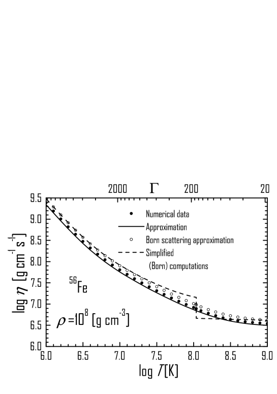
Figure 2: Temperature dependence of the shear viscosity for an iron plasma with the density $\rho=10^{8}$ g cm^-3 . The solid curve is the analytic approximation. Bold points present numerical calculations. Hollow circles correspond to the Born approximation. The dashed curve is the ”simplified” viscosity calculated in the Born approximation.

Figure 2 shows the temperature dependence of the shear viscosity for an iron plasma at $\rho=10^{8}$ g cm^-3 . The upper horizontal scale plots the Coulomb coupling parameter $\Gamma$. Bold points present our numerical results, while the solid curve shows the analytic approximation. The dashed curve is calculated with the simplified structure factor neglecting non-Born corrections. As in Fig. 1, the simplified viscosity displays jumps at the melting point, while the new results pass smoothly through this point. The charge number of iron ($Z=26$) is high enough for the non-Born corrections to be appreciable. To demonstrate this effect, hollow circles in Fig. 2 show the calculated viscosity in the Born approximation. We can see that the non-Born corrections reduce the viscosity by approximately 20%.

Figure 3: Shear viscosity at the temperature $T=10^{7}$ K as a function of the density for various chemical compositions (H, He, C, and Fe). Bold points are the numerical results and the curves show the analytic fit.

Figure 3 shows the density dependence of the shear viscosity for hydrogen, helium, carbon, and iron plasmas at $T=10^{7}$ K. We consider the densities typical for the cores of white dwarfs and the outer envelopes of neutron stars. Bold points show numerical results, and the curves are analytic approximations. The strong dependence of the viscosity on the chemical composition is due to the dependence of an electron-ion collision frequency on the charge number $Z$. In contrast to the thermal conductivity (see, e.g., Ref. [1]), the effect of electron-electron collisions on the viscosity is insignificant at the considered densities, even for hydrogen.

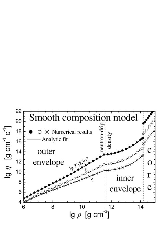
Figure 4: Shear viscosity of the ground-state matter versus $\rho$ for the three temperatures $T=10^{7}$, $10^{8}$, $10^{9}$ K. Solid curves show the analytic approximation; symbols are our numerical calculations. The vertical dotted lines indicate the neutron drip density and the crust-core interface in a neutron star (set to be $\rho=1.5\times 10^{14}$ g cm^-3 ). The electron shear viscosity in the stellar core, determined by scattering of electrons by degenerate protons, is presented for comparison.

Figure 4 demonstrates the density dependence of the shear viscosity in the density range from $10^{6}$ to $10^{15}$ g cm^-3 for the three temperatures $T=10^{7}$, $10^{8}$, $10^{9}$ K. The ground-state nuclear composition is employed with smoothed parameters. Symbols show the numerical results, and curves are analytic approximations. In contrast to the thermal conductivity [1], the shear viscosity decreases strongly with growing temperature. Note that the ratio $\rho/\eta$ grows with increasing density in the outer crust of a neutron star. These results are important for the damping of oscillations in the neutron star crust (see Section 3.3).

For illustrative purposes, the plot is continued beyond the crust into the stellar core (to densities $\rho\geq 1.5\cdot 10^{14}$ g cm^-3 ). In the core, we have used the equation of state of the matter presented in Ref. [29]. It is assumed that the core is composed of neutrons, protons, and electrons and is not superfluid. The electron viscosity in the core of such a star is mainly determined by the scattering of electrons by degenerate protons. The corresponding collision frequency is obtained in the same way as the electron-electron collision frequency (see Eq. (16)),

$$\nu_{\rm ep}=\pi^{2}\alpha^{2}\,\left(\frac{k_{\rm F}}{q_{0}}\right)\,\frac{\left(k_{\rm B}T\right)^{2}\,{m_{\rm p}^{\ast}}^{2}}{\hbar\,p_{\rm F}^{3}}\,c\approx 1.434\cdot 10^{12}\left(\frac{k_{\rm F}}{q_{0}}\right)\,T_{8}^{2}\left(\frac{m_{\rm p}^{\ast}}{m_{\rm p}}\right)^{2}\frac{n_{0}}{n_{\rm e}}\quad\mbox{c}^{-1},$$ (29)

where $m_{\rm p}$ is the proton mass, and $m^{\ast}_{\rm p}$ is its effective mass, which differs from $m_{\rm p}$ due to manybody effects (we have set $m_{\rm p}^{\ast}=0.7\,m_{\rm p}$). The Debye-screening parameter in the stellar core is

$$q_{0}^{2}=4\pi\,\sum_{j}e_{j}^{2}\,\frac{\partial n_{j}}{\partial\mu_{j}},$$ (30)

where the sum is taken over all types of charged particles (electrons and protons); $e_{j}$, $n_{j}$ and $\mu_{j}$ are the charge, number density, and chemical potential of particle species $j$. Owing to a strong suppression of the scattering rate by proton degeneracy, the electron viscosity in the core grows by a factor of $\sim 1000$ as compared to the viscosity in the crust.

3 P mode oscillations of a neutron star crust

This section is devoted to p mode oscillations (i.e., oscillations in which perturbations of the pressure dominate over the buoyant force) with high orbital numbers (multipolarity), $l\gtrsim 500$, localized in the outer crust of a nonrotating neutron star.

3.1 General formalism

3.1.1 Flat metric for the envelope of a nonrotating neutron star

The spacetime metric for a nonrotating neutron star [30] can be written as

$${\rm d}s^{2}=c^{2}{\rm e}^{2\Phi}\,{\rm d}\tilde{t}^{2}-{\rm e}^{2\lambda}\,{\rm d}r^{2}-r^{2}\,{\rm d}\Omega^{2},$$ (31)

where $\,{\rm d}\Omega^{2}=\,{\rm d}\theta^{2}+\sin^{2}\,\theta\,{\rm d}\varphi^{2}$, $\tilde{t}$ is the time coordinate, $r$ is the radial coordinate, $\theta$ and $\varphi$ are the polar and azimuthal angles, and the functions $\lambda(r)$ and $\Phi(r)$ determine spacetime curvature. It is sufficient to consider a thin envelope, neglecting the variation of the functions $\lambda(r)$ and $\Phi(r)$ in the crust and using their values at the stellar surface,

$${\rm e}^{2\Phi(R)}={\rm e}^{-2\lambda(R)}=1-\frac{2GM}{c^{2}R},$$ (32)

where $M$ is the gravitational stellar mass. Neglecting variations of $r$ in the envelope compared to the stellar radius $R$ (in the approximation of a thin envelope layer), we can rewrite Eq. (31) in the form

$${\rm d}s^{2}=c^{2}\left(1-\frac{R_{\rm G}}{R}\right)\,{\rm d}\tilde{t}^{2}-\left(1-\frac{R_{\rm G}}{R}\right)^{-1}\,{\rm d}r^{2}-R^{2}\,{\rm d}\Omega^{2},$$ (33)

where $R_{\rm G}=2GM/c^{2}\approx 2.953\,(M/M_{\odot})$ km is the gravitational radius. Introducing the local time $t$ and the local depth $z$,

$$t=\tilde{t}\,\sqrt{1-R_{\rm G}/R},\quad z=(R-r)/\sqrt{1-R_{\rm G}/R},$$ (34)

we come to a flat coordinate system in the neutron star crust,

$${\rm d}s^{2}=c^{2}\,{\rm d}t^{2}-\,{\rm d}z^{2}-R^{2}\,{\rm d}\Omega^{2}.$$ (35)

3.1.2 Equilibrium structure of the crust

The structure of a neutron star is determined by the equation of hydrostatic equilibrium, including the effects of General Relativity (the Tolman-Oppenheimer-Volkov equation; see, e.g., Ref. [30]). This equation is greatly simplified in the envelope; in the coordinate system (34) it can be written as

$$c_{\rm s}^{2}\frac{\,{\rm d}\rho_{0}}{{\rm d}z}=\frac{\,{\rm d}P_{0}}{{\rm d}z}=g\rho_{0},$$ (36)

where $P_{0}$ and $\rho_{0}$ are the equilibrium pressure and density, $c_{\rm s}^{2}\equiv{\partial P_{0}}/{\partial\rho_{0}}$ is the square of the local sound speed, and

$$g=\frac{GM}{R^{2}\sqrt{1-R_{\rm G}/R}}\approx\,1.327\cdot 10^{14}\frac{M}{M_{\odot}}\left(\frac{10\,\mbox{km}}{R}\right)^{2}\left/\sqrt{1-R_{\rm G}/R}\right.\quad\frac{\mbox{cm}}{\mbox{s}^{2}}$$ (37)

is the gravitational acceleration.

In computations we have used the equation of state of a fully degenerate electron gas with electrostatic corrections and have employed the model of the ground-state matter with smoothed parameters. Alternatively, we have used a polytropic envelope, composed of ⁵⁶Fe nuclei, where the pressure is determined by degenerate electrons, assumed to be relativistic at all densities.

3.1.3 The oscillation equation

In the outer envelopes of neutrons stars, the main contribution to the pressure is produced by degenerate electrons. Therefore, while considering p-modes, we can use a single equation of state to describe the equilibrium configuration of the star and perturbations.

Let us use the Euler equation in a flat-space metric (35),

$${\frac{\partial{\bm{U}}}{\partial{t}}}+({\bm{U}}\cdot\nabla){\bm{U}}=-\frac{\nabla P}{\rho}+{\bm{g}},$$ (38)

where $P$ is the pressure. The continuity equation must also be satisfied,

$$\frac{\partial\rho}{\partial t}+\nabla\left(\rho{\bm{U}}\right)=0.$$ (39)

Assuming that the velocity $\bm{U}$ is small and introducing Euler perturbations of the pressure $\delta P=P-P_{0}$ and the density $\delta\rho=\rho-\rho_{0}$, we obtain the linearized Euler equation

$${\frac{\partial{\bm{U}}}{\partial t}}=\frac{\delta\rho}{\rho_{0}^{2}}\,\nabla P_{0}-\frac{1}{\rho_{0}}\,\nabla\delta P,$$ (40)

and the continuity equation

$$\frac{\partial\delta\rho}{\partial t}+\nabla\left(\rho_{0}{\bm{U}}\right)=0,$$ (41)

while the equation of state for the perturbations can be rewritten in the form

$$\delta P=c_{\rm s}^{2}\delta\rho.$$ (42)

We will consider irrotational motion and write the velocity in the form ${\bm{U}}=\nabla\phi$, where $\phi$ is the velocity potential, which is a scalar function of coordinates and time. Formally, the function $\phi$ is determined up to an arbitrary function of time, which we choose in such a way that the Euler equation can be rewritten (using Eqs. (36) and (42)) as

$$\frac{\partial\phi}{\partial t}=-\frac{\delta P}{\rho_{0}}=-c_{\rm s}^{2}\frac{\delta\rho}{\rho_{0}}.$$ (43)

Differentiating (43) with respect to $t$ and taking into account Eqs. (41) and (36), we get

$$\frac{\partial^{2}\phi}{\partial t^{2}}=c_{\rm s}^{2}\Delta\phi+{\bm{g}}\cdot\nabla\phi,$$ (44)

where we have introduced the Laplace operator

$$\Delta\approx{\frac{\partial{{}^{2}}}{\partial{z^{2}}}}+\frac{1}{R^{2}}\left({\frac{\partial{{}^{2}}}{\partial{\theta^{2}}}}+\frac{1}{\sin^{2}\theta}{\frac{\partial{{}^{2}}}{\partial{\varphi^{2}}}}\right).$$ (45)

An equation that coincides with (44) was obtained by Lamb [31] for oscillations in the Earth atmosphere. The variables in (44) can be separated if we write

$$\phi={\rm e}^{\imath\omega t}\,Y_{lm}(\theta,\varphi)\,F(z),$$ (46)

where $\omega$ is the oscillation frequency, $Y_{lm}(\theta,\varphi)$ is a spherical harmonic function (see, e.g., Ref. [32]), and $F(z)$ is an unknown function of the depth determined by

$${\frac{{\rm d}{{}^{2}F}}{{\rm d}{z^{2}}}}+\frac{g}{c_{\rm s}^{2}}{\frac{{\rm d}{F}}{{\rm d}{z}}}+\left(\frac{\omega^{2}}{c_{\rm s}^{2}}-\frac{l(l+1)}{R^{2}}\right)F=0.$$ (47)

The first boundary condition for this equation,

$$\mbox{function }F(z)\mbox{ is bounded as }z\rightarrow 0,$$ (48)

follows from the requirement of a finite oscillation amplitude at the stellar surface. The second boundary condition is imposed artificially. In the current study, we have to solve equations that are applicable only in the thin stellar crust. Therefore, oscillations should be damped at sufficiently high depths. For simplicity, we formally move this boundary condition to infinity along $z$ and will check a true localization of oscillations (see Section 3.3). In this case, the second boundary condition can be written

$$F(z)\rightarrow 0~{}\mbox{ as }z\rightarrow\infty.$$ (49)

Together with the boundary conditions (48) and (49), Eq. (47) specifies eigenfrequencies and eigenmodes of oscillations. Moreover, the following asymptotes are valid at large and small depths:

$$F(z)\propto\left\{\begin{array}[]{ll}1-\omega^{2}z/g&z\rightarrow 0,\\ \exp\left(-\sqrt{l(l+1)}\,z/R\right)&z\rightarrow\infty.\end{array}\right.$$ (50)

Perturbations of the pressure and the density are expressed in terms of the function $\phi(r)$ using Eq. (43),

$$\delta P=-\imath\omega\,\rho_{0}\,\phi,\quad\delta\rho=\frac{\delta P}{c_{\rm s}^{2}}=-\imath\frac{\omega\,\rho_{0}}{c_{\rm s}^{2}}\,\phi.$$ (51)

Due to the boundary condition (48), variations of the pressure and the density, $\delta P$ and $\delta\rho$, vanish at the stellar surface (because $\rho_{0}(R)=0$). We can see from these last expressions that the number of radial nodes ($k$) of the velocity potential coincides with the number of nodes of the pressure and density variations. Below, we will call $k$ the number of radial nodes of the mode.

The displacement vector for an oscillating matter element can be written in the form

$${\bm{\xi}}\equiv\int{\bm{U}}\,{\rm d}t=-\frac{\imath}{\omega}\,\nabla\cdot\phi.$$ (52)

The z component of this vector is

$$\xi_{z}=-\frac{\imath}{\omega}\,Y_{lm}(\theta,\varphi)\,{\frac{{\rm d}{F}}{{\rm d}{z}}},$$ (53)

and the magnitude of horizontal displacement can be estimated as

$$\left|\xi_{\rm h}\right|\approx\frac{l}{\omega\,R}\,\left|F(z)\right|.$$ (54)

The quantities $lF(z)/R$ and ${\rm d}F/{\rm d}z$ appear in Eq. (47) on equal footing. Therefore, horizontal and radial displacements should have the same order of magnitude for the oscillations considered.

Oscillations of a polytropic envelope in a plane-parallel approximation were studied earlier by Gough [33] assuming that the equations of state of the unperturbed matter and the perturbations are polytropic with different indices. In the limiting case of the same polytropic index $n$, his result can be presented as follows. The mode containing $k$ radial nodes has the eigenfrequency

$$\omega^{2}_{k}=\frac{g}{R}\,\sqrt{l(l+1)}\,\left(\frac{2k}{n}+1\right)\,\approx 10^{8}\,g_{14}\,\left(\frac{10\,\mbox{km}}{R}\right)\,\sqrt{l(l+1)}\,\left(\frac{2k}{n}+1\right)~{}~{}\mbox{s}^{-2},$$ (55)

while the velocity potential is given by

$$F_{k}(z)=\exp\left(-\sqrt{l(l+1)}\,\frac{z}{R}\right)L_{k}^{(n-1)}\left(2\,\sqrt{l(l+1)}\,\frac{z}{R}\right),$$ (56)

where $L_{k}^{(n-1)}(x)$ is a generalized Laguerre polynomial (see, e.g., Ref. [28]) and $g_{14}$ is the gravitational acceleration at the stellar surface in units of $10^{14}$ cm s^-2. Note that the eigenfrequencies agree with the simple estimate $\omega^{2}\sim g/a$, where $a\sim R/l$ is the characteristic depth for the oscillation localization.

Let us remark that the mode with $k=0$, which does not have any radial nodes, corresponds to the vanishing Lagrangian variations of the pressure and the density ($\nabla\cdot{\bm{U}}$=0, see (71)); its parameters do not depend on the polytropic index. Adding the condition $\nabla\cdot{\bm{U}}\equiv\Delta\phi=0$ to Eq. (44), it is easy to show that this mode is described by the function $F(z)=\exp\left(-\sqrt{l(l+1)}z\,/R\right)$ and has the frequency

$$\omega_{0}^{2}=\frac{g}{R}\,\sqrt{l(l+1)}\approx 10^{8}\,g_{14}\,\left(\frac{10\,\mbox{km}}{R}\right)\,\sqrt{l(l+1)}~{}~{}\mbox{s}^{-2};$$ (57)

it exists for any equation of state. Therefore, the frequency $\omega_{0}$ will further be used to normalize oscillation frequencies.

The frequencies $\omega$ we discuss refer to the coordinate system of the stellar envelope (see Eq. (34)). They are easily transformed to the frequencies $\widetilde{\omega}$ detected by a distant observer,

$$\widetilde{\omega}=\omega\,\sqrt{1-R_{\rm G}/R}.$$ (58)

3.2 Viscous damping of oscillations

In this section, we consider the damping of oscillations with velocity potentials of the form ${\rm e}^{\imath\omega t}\,Y_{lm}(\theta,\varphi)F(z)$ in a spherically symmetric star under the action of shear viscosity. We take flat space-time metric which is applicable to oscillations studied in Section 3.1. This is because the flat metric (35), which coincides with the metric for a thin spherical layer in a flat space-time, can be introduced in the region, where oscillations are localized. As a result, it is sufficient to consider the oscillation damping time in a flat metric and transform this time (in accordance with Eq. (34)) into the frame of a distant observer. We define the oscillation damping time $\tau$ as

$$\tau=E/|{\rm d}E/{\rm d}t|,$$ (59)

where

$$E=\int\varepsilon\,{\rm d}V=\int\rho\,\frac{|U|^{2}}{2}\,{\rm d}V$$ (60)

is the total energy of oscillations and

$$\varepsilon=\frac{1}{4}\left(\rho_{0}\,|U|^{2}+\frac{c_{\rm s}^{2}}{\rho_{0}}\,|\delta\rho|^{2}\right)$$ (61)

is the energy density of oscillations at a given point averaged over an oscillation period (see, e.g., Ref. [34]). The additional factor of $1/2$ in the expression for $\varepsilon$ is required due to the averaging over the oscillation period. The integration is carried out over the entire volume of the star (in practice, over the region where the oscillations are localized). We neglect perturbations of the gravitational potential. The last equality in Eq. (60) is determined by the equality of the mean kinetic and potential energies for low-amplitude harmonic oscillations. Note that some authors introduce the damping time for the oscillation amplitude rather than the damping time (59) for the oscillation energy.

When calculating the energy from Eq. (60), the angular integration can be carried out analytically,

$$E=\frac{1}{2}\int_{0}^{R}\rho\left[\left(F\,^{\prime}\right)^{2}+\frac{l(l+1)}{r^{2}}F^{2}\right]r^{2}\,{\rm d}r.$$ (62)

The period-averaged rate of the viscous energy dissipation is (see, e.g., Ref. [34])

$$\frac{\,{\rm d}E}{\,{\rm d}t}=-\frac{1}{4}\int\sigma_{ik}^{\prime}\left(\frac{\partial U_{i}^{\ast}}{\partial x_{k}}+\frac{\partial U_{k}^{\ast}}{\partial x_{i}}\right)\,{\rm d}V,$$ (63)

where the viscous stress tensor $\sigma_{\alpha\beta}^{\prime}$ is given by Eq. (8). As in the expression for the oscillation energy $E$, the additional factor of $1/2$ is required owing to averaging over the oscillation period. It is easy to see that the energy dissipation rate separates into a sum of terms associated with shear and bulk viscosities. We will restrict ourselves to the dissipation determined by the shear viscosity. The integration over the angular variables in Eq. (63) can be carried out analytically (see the Appendix).

3.3 Discussion of numerical results

As an example, let us choose a ”canonical” model for a neutron star with the mass $M=1.4M_{\odot}$ and the radius $R=10$ km. For this model,

$$\omega_{0}\approx 1.56\cdot 10^{5}\left(\frac{l(l+1)}{10^{4}}\right)^{1/4}\,\mbox{s}^{-1}$$ (64)

and for a distant observer

$$\widetilde{\omega}_{0}\approx 0.766\,\omega_{0}\approx 1.19\cdot 10^{5}\left(\frac{l(l+1)}{10^{4}}\right)^{1/4}\mbox{~{}s}^{-1}.$$ (65)

The thickness of the outer crust in such a star ($\rho<4\cdot 10^{11}$ g$\cdot$cm^-3, before the neutron drip point) is $\approx 364$ m.

Oscillation eigenfrequencies have been found via a series of iterative trials, checking for the coincidence of a mode number with a number of radial nodes.

3.3.1 Oscillation eigenfrequencies

Figure 5: Eigenfrequencies of oscillations localized in the crust of a ”canonical” neutron star. The frequencies are normalized to the frequency $\omega_{0}$ given by Eq. (57). The numbers next to the curves indicate the number of radial nodes.

Figure 6: Frequencies of oscillations localized in the crust of a ”canonical” neutron star as detected by a distant observer. The subscript of $f$ denotes the number of radial nodes.

The dependence of oscillation eigenfrequencies on $l$, calculated from Eq. (47) with the boundary conditions (48) and (49), is presented in Figs. 5 and 6. As mentioned earlier, the frequency of the fundamental mode, which does not have any radial nodes, is determined by Eq. (57) for all $l$. With decreasing $l$, oscillations penetrate deeper into the outer crust, where the equation of state is softened because the electron gas becomes relativistic and electrons undergo beta captures. This slightly decreases the dimensionless eigenfrequencies. As in the model with the polytropic equation of state (see Eq. (55)), the separation between squares of neighboring eigenfrequencies for any $l$ is nearly constant. A weak decrease of this separation with the growing number of radial nodes is due to the penetration of oscillations into deeper layers of the star, where the equation of state is softer. When $l\sim 500$, the main oscillation energy is localized in the region 50 m$\lesssim\,z\,\lesssim$ 400 m, where the equation of state of the degenerate, relativistic electron gas well describes the profile of the sound speed. Therefore, the estimate (55) for eigenfrequencies of the polytropic crust model with the polytropic index $n=3$ is justified (deviations constitute several per cent).

3.3.2 Oscillation eigenmodes

Figure 7: Root-mean-square (over angles) amplitude of radial displacements of matter for modes with $l=500$. The subscript of $\xi$ indicates the number of radial nodes. The root-mean-square amplitude of radial displacements at the stellar surface has been set equal to 1 m.

Figure 7 presents profiles of radial displacements of matter elements for the modes with $l=500$. The root-mean-square amplitude of radial displacements of the stellar surface has been set 1 m. Since we are studying linear oscillations, this quantity is an arbitrary (sufficiently small) constant that normalizes the solution. From Fig. 7 one can easily determine the magnitude of radial displacements in the star for any other amplitude of the displacements at the surface. With growing $z$, the radial displacement amplitude $\xi_{z}$ overall decreases. At $z\sim 300$ m, the decrease becomes monotonic and gradually tends to the exponential asymptotic (50). This means that oscillations are localized in the outer crust.

Figure 8: Angle-averaged energy density $\varepsilon$ of oscillations with $l=500$. The subscript of $\varepsilon$ indicates the number of radial nodes. The root-mean-square amplitude of radial displacements at the stellar surface is 1 m.

This effect is manifested even more clearly in the energy density of oscillations. Figure 8 presents the dependence of the angle-averaged energy density $\varepsilon$ versus depth $z$ for oscillations with $l=500$. The mode amplitude is normalized in the same way as in Fig. 7. In our approximation, the energy density is proportional to the square of the normalized amplitude of radial surface displacements. The depicted modes are localized in the outer crust of the star. The energy density of oscillations varies relatively weakly within the ”critical” depth $z\lesssim 100-200$ m, after which it falls off exponentially. The energy density decreases by more than two orders of magnitude near the boundary between the outer and inner crusts.

Figure 9: Angle-averaged energy density $\varepsilon$ of oscillations with $l=500$. The subscript of $\varepsilon$ indicates the number of radial nodes. The curves refer to the polytropic model, and the symbols are for the exact equation of state.

As noted in Section 3.3.1, at $l\sim 500$ oscillation frequencies are well reproduced by a polytropic crust model. The situation is somewhat different for oscillation eigenmodes. Normalization at the stellar surface is not expedient for these modes, since the polytropic model poorly reproduces the structure of the star at low depths, $z\lesssim 40$ m. Consequently, such a normalization leads to large errors at the depths of interest to us, $z\lesssim 100-200$ m, where the main oscillation energy is concentrated. Therefore, we need a special normalization to compare exact and polytropic modes. Figure 9 (similar to Fig. 8) shows the angle-averaged energy density $\varepsilon$ of oscillations as a function of $z$. The symbols refer to exact numerical results, while the curves are for the polytropic model, normalized in such a way to be in agreement with the exact results in the region where oscillations are localized. We can conclude that the polytropic model for the outer crust satisfactorily reproduces the energy density of oscillations at depths of 60 m $\lesssim\,z\,\lesssim\,300$ m for modes with $l\lesssim 500$.

3.3.3 The oscillation damping

Figure 10: Damping time $\tau$ of oscillations for a distant observer as a function of multipolarity $l$ for a neutron star with the internal temperature $T=10^{7}$ K. The subscript of $\tau$ gives the number of radial nodes.

Figure 11: Same as Fig. 10 but for the internal temperature $T=10^{8}$ K.

Figure 12: Same as Fig. 10 but for the internal temperature $T=10^{9}$ K.

In our calculations we have considered the neutron star crust as isothermal. This approximation describes well the internal temperature profile. The temperature is nearly independent of depth due to a high thermal conductivity of degenerate electrons. Naturally, oscillation frequencies and damping times do not depend on the normalization amplitude (the amplitude of radial surface displacements). Figures 10, 11 and 12 present the dependence of the oscillation damping time $\tau$ (for a distant observer) on $l$ for a canonical neutron star with the internal temperature $T=10^{7},$ $10^{8}$, and $10^{9}$ K. The strong temperature dependence of the damping time is due to the appreciable decrease of the viscosity with increasing temperature (Fig. 4). The damping time can be estimated from characteristic oscillation parameters as

$$\tau\sim\varepsilon/{\dot{\varepsilon}}\sim\rho U^{2}\left/\left(\eta\left(\frac{U}{\lambda}\right)^{2}\right)\right.\sim\lambda^{2}\frac{\rho}{\eta},$$ (66)

where $\dot{\varepsilon}$ is the local viscous dissipation rate, while $U$ and $\lambda$ are, respectively, the characteristic velocity and its variation length scale in the region of oscillation localization.

Let us consider Fig. 11 in more detail. Oscillations with $l\sim 500$ are localized at $z\lesssim 100$ m (Fig. 8), which corresponds to densities $\rho\lesssim 10^{10}$ g cm^-3 . Under these conditions, the ratio $\rho/\eta$ is $\sim 3$ s cm^-2 (Fig. 4) and grows with increasing $l$ (due to the decrease of the density in the region of oscillation localization). Let us make estimates for the modes with $l\sim 500$. The velocity variation length scale can be estimated as $\lambda\sim R/l$. Note that this scale decreases for modes with a large number of radial nodes, accelerating the damping of these oscillations. For the fundamental mode (without any radial nodes), the damping time (in the frame of a distant observer) can be estimated as

$$\tau\sim 1.2\,10^{4}\,\times(500/l)^{2}\mbox{ s}\approx 120\times(500/l)^{2}\mbox{~{}day},$$ (67)

in good agreement with the numerical results for $l\sim 500$. The damping time drops weaker than $\propto l^{-2}$ because the ratio $\rho/\eta$ grows for higher $l$, owing to the decrease of the density in the region of oscillation localization.

For the outer crust of a star with the temperature $T=10^{9}$ K, the ratio $\rho/\eta$ depends weakly on $\rho$. Therefore, the oscillation damping time obeys the law $\tau\propto l^{-2}$.

Figure 13: Damping time of oscillations as a function of the internal neutron star temperature for modes with $l=500$. The subscript indicates the number of radial nodes. Numerical results are redshifted for a distant observer.

The damping time as function of the crust temperature is presented in Fig. 13, where we have chosen the modes with $l=500$ as an example. The damping time grows by approximately two orders of magnitude as the temperature varies from $10^{7}$ to $10^{8}$ K. When the temperature increases by another order of magnitude, the damping time grows further by a factor of three. This is due to the nonlinear decrease of the viscosity with the growth of $T$ (Fig. 4).

There are many other oscillation damping mechanisms [14], in addition to the viscous damping considered here. For example, one often considers the damping due to the emission of gravitational and electromagnetic waves (for oscillations of the stellar matter with a frozen-in magnetic field). In our case, these mechanisms are inefficient due to high multipolarity, $l\sim 500$. If $l$ is high, we expect gravitational or electromagnetic radiation to be generated by an ensemble of closely spaced coherent elementary radiating regions, which radiate in antiphase and cancel one another. Formally, the weakness of this radiation is manifested by the presence of large factors $(2l+1)!!$ in the denominators of the expressions for the radiation intensities (see, e.g., Refs. [35, 36]). An analysis shows that the damping of oscillations we consider here is determined to a great extent by the shear viscosity.

A detailed analysis of the evolution of pulse shapes of some radio pulsars provides an evidence that high-multipole oscillations are, indeed, excited in them (see, e.g., the recent paper [37]). However, reliable observational data on the existence of such oscillations have not yet been obtained.

4 Conclusions

We have calculated the shear viscosity of dense stellar matter for a broad range of temperatures and densities typical for the cores of white dwarfs and the envelopes of neutron stars. We have considered the matter composed of astrophysically important elements, from H to Fe, at the densities from $10^{2}-10^{4}$ g cm^-3 to $10^{7}-10^{10}$ g cm^-3 . At higher densities, $10^{10}-10^{14}$ g cm^-3 , we used the model for the cold ground-state matter taking into account finite sizes of atomic nuclei and the distribution of proton charge within the nuclei. Under the conditions described above, the shear viscosity is determined by Coulomb scattering of degenerate electrons by atomic nuclei. We have used the modified structure factor of ions proposed by Baiko et al. [22] and applied by Potekhin et al. [1] for calculating the thermal and electrical conductivities of dense matter. In the ion liquid, this modification approximately takes into account a quasi-ordering in ions positions, which reduces the electron-ion scattering rate. In the crystalline phase, the new structure factor takes into account multi-phonon processes, which are important near the melting temperature $T_{m}$. The new results near the melting point differ appreciably from the results of Flowers and Itoh [2, 3] obtained for a Coulomb liquid. We have approximated our numerical results by an analytic expression convenient for applications.

We have analyzed eigenfrequencies and eigenmodes of oscillations localized in the outer crust of a neutron star (in the plane-parallel approximation). A polytropic model for the crust can reasonably well reproduce the eigenfrequencies of oscillation modes with multipolarity $l\sim 500$. We have also calculated viscous damping times of the oscillations. We have obtained a sharp decrease in the damping time with decreasing the internal temperature of a neutron star. For example, for a neutron star with mass $M=1.4M_{\odot}$, radius $R=10$ km, and the internal temperature $T=10^{8}$ K, the damping time for the fundamental mode with $l=500$ is $\sim 160$ days. When the temperature decreases to $T\sim 10^{7}$ K, the damping time falls to $\sim 15$ days.

In our calculations, we have used the model of the ground-state matter in the neutron star crust with a smoothed dependence of the parameters of atomic nuclei on the density of the matter. More accurate calculations would require a more detailed model of the ground-state matter, where the composition varies with depth in a jump-like manner (showing a series of weak first-order phase transitions at some depths). The presence of these jumps could amplify the damping of the oscillations. We plan to consider this problem in the future.

Acknowledgments

We thank D. Gough for reprints of his papers on oscillations of polytropic stellar envelopes, and W. Dziembowski, who pointed out these works to us. We are also grateful to K.P. Levenfish and A.Y. Potekhin for useful discussions. This work was supported by a student grant of the Non-Profit Foundation ”Dynasty” and the International Center for Fundamental Physics in Moscow, the Russian Foundation for Basic Research (RFFI-IAU grant no. 03-02-06803 and project no. 05-02-16245), and the Program of Support for Leading Scientific Schools of Russia (NSh-1115.2003.2).

Appendix. The integration of the viscous dissipation rate of oscillation energy over angular variables

While calculating the angular integral in Eq. (63), it is convenient to introduce the notation

$$\widetilde{\sigma}_{ik}\equiv\frac{\partial U_{i}}{\partial x_{k}}+\frac{\partial U_{k}}{\partial x_{i}}.$$ (68)

Then, the part of Eq. (63), associated with the shear viscosity, can be written as

$$\frac{{\rm d}E}{{\rm d}t}=-\frac{1}{4}\int_{0}^{R}\,\eta\,r^{2}\,{\rm d}r\int\left[\widetilde{\sigma}_{ik}\widetilde{\sigma}_{ki}^{\ast}-\frac{4}{3}\left|\nabla{\bm{U}}\right|^{2}\right]\,{\rm d}\Omega=-\frac{1}{4}\int_{0}^{R}r^{2}\,\eta\left(I_{1}-\frac{4}{3}I_{2}\right)\,{\rm d}r,$$ (69)

where $\,{\rm d}\Omega$ is a solid angle element,

$$I_{1}\equiv\int\widetilde{\sigma}_{ik}\widetilde{\sigma}_{ki}^{\ast}\,{\rm d}\,\Omega\quad\mbox{and}\quad I_{2}\equiv\int\left|\nabla{\bm{U}}\right|^{2}\,{\rm d}\Omega.$$ (70)

Here, we have assumed that the unperturbed star is spherically symmetric, so that the shear viscosity does not depend on angular variables. The integrals $I_{1}$ and $I_{2}$ have been taken analytically for the hydrodynamic velocities of the form ${\bm{U}}=\nabla\phi$, where the velocity potential is $\phi={\rm e}^{\imath\omega t}Y_{lm}(\theta,\varphi)F(r)$.

The integral $I_{1}$ can be taken if we write the components of the tensor $\widetilde{\sigma}_{ik}$ in spherical coordinates (see, e.g., Ref. [34]). After this, the angular integration is carried out analytically (using the properties of the function $Y_{lm}(\theta,\varphi)$; see, e.g., Ref. [32]). This yields

$$I_{1} = 4\,\left\{\left(F^{\prime\prime}\right)^{2}+2\,\frac{1+l(l+1)}{r^{2}}\,\left(F\,^{\prime}\right)^{2}-6\,\frac{l(l+1)}{r^{3}}\,F\,^{\prime}F+l(l+1)\,\frac{1+l(l+1)}{r^{4}}\,F^{2}\right\}$$

$$\approx 4\,\left\{\left(F^{\prime\prime}\right)^{2}+2\,\frac{l(l+1)}{R^{2}}\,\left(F\,^{\prime}\right)^{2}+l(l+1)\,\frac{l(l+1)}{R^{4}}\,F^{2}\right\},$$

where the last equality is valid in the approximation of plane-parallel layer.

Let us now consider the integral $I_{2}$. For this purpose, we write the divergence of the velocity

$$\nabla{\bm{U}} = \Delta\phi=\left(\frac{1}{r^{2}}\,{\frac{\partial{}}{\partial{\,r}}}\,r^{2}\,{\frac{\partial{\,F}}{\partial{\,r}}}\,Y_{lm}(\theta,\varphi)+F\,\Delta_{\Omega}\,Y_{lm}(\theta,\varphi)\right)\,{\rm e}^{\imath\omega t}$$ (71)

$$= \left(F^{\prime\prime}+\frac{2\,F\,^{\prime}}{r}-\frac{l(l+1)}{r^{2}}\,F\right)\,Y_{lm}(\theta,\varphi)\,{\rm e}^{\imath\omega t},$$

where $\Delta_{\Omega}$ is the angular part of the Laplacian. The integral $I_{2}$ is easily calculated,

$$I_{2}=\left(F^{\prime\prime}+\frac{2\,F\,^{\prime}}{r}-\frac{l(l+1)}{r^{2}}\,F\right)^{2}\approx\left(F^{\prime\prime}-\frac{l(l+1)}{R^{2}}\,F\right)^{2},$$ (72)

where the last equality is valid in the plane-parallel layer approximation. As expected, Eq. (69) does not depend on the azimuthal number $m$ (due to the spherical symmetry of the unperturbed star). It can be shown that ${\rm d}E/{\rm d}t\geq 0$ for all allowed values $l=0,\,1,\,2,\ldots$

References

- [1] A.Y. Potekhin, D.A Baiko., P. Hansel, and D.G. Yakovlev, A&A, 346, 345 (1999).
- [2] E. Flowers, N. Itoh, Astrophysical Journal, 206, 218 (1976).
- [3] E. Flowers and N. Itoh., Astrophysical Journal, 230, 847 (1979).
- [4] R. Nandkumar and C.J. Pethick, MNRAS, 209, 511 (1984).
- [5] N. Itoh, Y. Kohyama, N. Matsumoto, and M. Seki, Astrophysical Journal, 285, 758 (1984).
- [6] N. Itoh, H. Hayashi, and Y. Kohyama, Astrophysical Journal, 418, 405 (1993).
- [7] K.S. Thorne and A. Campolattaro, Astrophysical Journal, 149, 591 (1967).
- [8] R. Price, K.S. Thorne, Astrophysical Journal, 155, 163 (1969).
- [9] K.S. Thorne, Astrophysical Journal, 158, 1 (1969).
- [10] K.S. Thorne, Astrophysical Journal, 158, 997 (1969).
- [11] A. Campolattaro and K.S. Thorne, Astrophysical Journal, 159, 847 (1970).
- [12] J.R. Ipser and K.S. Thorne, Astrophysical Journal, 181, 181 (1973).
- [13] P.N. McDermott, H.M. Van Horn, and J.F. Scholl, Astrophysical Journal, 268, 837 (1983).
- [14] P.N. McDermott, H.M. Van Horn, and C.J. Hansen, Astrophysical Journal, 325, 725 (1988).
- [15] N. Stergioulas, Living Rev. in Relativity, 6, 3 (2003).
- [16] V.M. Kaspi, in Young Neutron Stars and Their Environments, edited by F. Camilo and B.M. Gaensler (Astronomical Society of the Pacific, San Francisco, 2004), pp. 231–238.
- [17] H. DeWitt, W. Slattery, D. Baiko, D. Yakovlev, Contrib. Plasma Phys., 41, 251 (2001).
- [18] L.D. Landau and E.M. Lifshitz, Theory of Elasticity, Pergamon Press, Oxford, 1986.
- [19] J.M. Ziman, Electrons and Phonons, Clarendon, Oxford, 1960.
- [20] D.A. Baiko and D.G. Yakovlev, Astron. Lett. 21, 702 (1995).
- [21] V.B. Berestetskii, E.M. Lifshitz, and L.P. Pitaevskii, Quantum Electrodynamics, Pergamon Press, Oxford, 1982.
- [22] D.A. Baiko, A.D. Kaminker, A.Y. Potekhin, and D.G. Yakovlev, Phys. Rev. Lett., 81, 5556 (1998).
- [23] D.G. Yakovlev, Sov. Astron. 31, 347 (1987).
- [24] A.Y. Potekhin, G. Chabrier, and D.G. Yakovlev, A&A, 323, 415 (1997).
- [25] B. Jancovici, Nuovo Cim., 25, 428 (1962).
- [26] A.D. Kaminker, C.J. Pethick, A.Y. Potekhin, V. Thorsson, D.G. Yakovlev, A&A, 343, 1009 (1999).
- [27] O.Y. Gnedin, D.G. Yakovlev, and A.Y. Potekhin, MNRAS, 324, 725 (2001).
- [28] M. Abramowitz and I.A. Stegun, Handbook of Mathematical Functions, Ed. by M. Abramowitz and I.A. Stegun, Dover, New York, 1971.
- [29] M. Prakash, T.L. Ainsworth, and J.M. Lattimer, Phys. Rev. Lett., 61, 2518 (1988).
- [30] S.L. Shapiro and S.A. Teukolsky, Black Holes, White Dwarves, and Neutron Stars: The Physics of Compact Objects, Wiley, New York, 1983.
- [31] H. Lamb, Proc. Roy. Soc. A, 84, 551 (1911).
- [32] D.A. Varshalovich, A.N. Moskalev, and V.K. Khersonskii, Quantum Theory of Angular Momentum, World Sci., Singapore, 1988.
- [33] D.O. Gough, in Astrophysical fluid dynamics, Ed. J-P. Zahn & J. Zinn-Justin (Elsevier, for Les Houches Session XLVII, Amsterdam, 1993), pp. 399–560.
- [34] L.D. Landau and E.M. Lifshitz, Fluid Mechanics, Pergamon Press, Oxford, 1987 .
- [35] E. Balbinski and B.F. Schutz, MNRAS, 200, 43 (1982).
- [36] P.N. McDermott, M.P. Savedoff, H.M. Van Horn, E.G. Zweibel, C.J. Hansen, Astrophysical Journal, 281, 746 (1984).
- [37] J. Clemens and R. Rosen, Astrophysical Journal, 609, 340 (2004).