On the spin-up/spin-down transitions in accreting X-ray binaries

Abstract

Accreting X-Ray Binaries display a wide range of behaviours. Some of them are observed to spin up steadily, others to alternate between spin-up and spin-down states, sometimes superimposed on a longer trend of either spin up or spin down. Here we interpret this rich phenomenology within a new model of the disk-magnetosphere interaction. Our model, based on the simplest version of a purely material torque, accounts for the fact that, when a neutron star is in the propeller regime, a fraction of the ejected material does not receive enough energy to completely unbind, and hence falls back into the disk. We show that the presence of this feedback mass component causes the occurrence of multiple states available to the system, for a given, constant value of the mass accretion rate $\dot{M}_{*}$ from the companion star. If the angle $\chi$ of the magnetic dipole axis with respect to the perpendicular to the disk is larger than a critical value $\chi_{\rm crit}$, the system eventually settles in a cycle of spin-up/spin-down transitions for a constant value of $\dot{M}_{*}$ and independent of the initial conditions. No external perturbations are required to induce the torque reversals. The transition from spin up to spin down is often accompanied by a large drop in luminosity. The frequency range spanned in each cycle and the timescale for torque reversals depend on $\dot{M}_{*}$, the magnetic field of the star, the magnetic colatitude $\chi$, and the degree of elasticity regulating the magnetosphere-disk interaction. The critical angle $\chi_{\rm crit}$ ranges from $\sim 25^{\circ}-30^{\circ}$ for a completely elastic interaction to $\sim 40^{\circ}-45^{\circ}$ for a totally anelastic one. For $\chi\lesssim\chi_{\rm crit}$, cycles are no longer possible and the long-term evolution of the system is a pure spin up. We specifically illustrate our model in the cases of the X-ray binaries GX 1+4 and 4U 1626-67.

1 Introduction

Accreting X-ray binaries, with luminosities up to $\sim 10^{38}-10^{39}$ erg/s, constitute the brightest X-ray sources in the sky. Since their discovery (Giacconi et al. 1971) more than three decades ago, they have provided a unique laboratory to study, among other things, the physical processes regulating accretion onto a strongly magnetized neutron star (typically, $B\gtrsim 10^{11}$ G). In neutron star (NS) binary systems containing a supergiant or a low-mass star, mass transfer takes place through Roche Lobe overflow, and the specific angular momentum of matter is sufficiently high to form an accretion disk (the conditions for forming a disk are however not necessarily met in Be-star systems, where the NS accretes from capturing the star’s wind; e.g. Rappaport 1982; Henrichs 1983). In disk-fed systems that host a strongly magnetic neutron star, the material from the disk is channelled toward the magnetic poles, where it releases its gravitational energy giving rise to the X-ray luminosity we observe. Pulsations at the neutron star spin frequency are thus generated from a lighthouse-like effect. While the luminosity yields an estimate of the mass accretion rate, pulse timing measurements allow one to measure the torque, and hence probe the nature of the accretion process mediated by the magnetosphere of the star. Early works (Pringle & Rees 1972; Davidson & Ostriker 1973; Lamb, Pethick & Pines 1973) showed that, when accretion occurs through a prograde disk, the angular momentum transferred by the accreting material to the star (material torque) tends to spin the star up, until the centrifugal barrier inside the corotation radius of the magnetosphere (Illianorov & Sunyaev 1975) becomes large enough to inhibit further accretion. The star is then expected to settle in a state with an equilibrium spin period which depends mainly on the mass accretion rate provided by the companion and the neutron star magnetic field (e.g. Frank, King & Raine 2003).

Observations of disk-accreting X-ray pulsars during the 1970s and 1980s were rather sparse, and appeared to be roughly compatible with the near-equilibrium picture (e.g. Nagase 1989), although there were already hints at times of some unexpected behaviours. These included torque reversals for some time while still accreting, or spin up rates much smaller than expected for the observed luminosity. In the 1990s, continuous monitoring of several disk-fed X-ray pulsars with the Burst and Transient Source Experiment (BATSE) on board the Compton Gamma-Ray observatory, shed light on the long-term behaviour of several objects (see Bildsten et al. 1997 for a comprehensive review). Particularly striking were the findings for GX 1+4 and 4U 1626-67: after about 15 years (for GX 1+4) and 20 years (for 4U 1626-67) of spin up, both systems showed a torque reversal, which made them switch to a spin-down phase. Other systems, like Cen X-3, Vela X-1, Her X-1, often showed an alternation of spin up and down sometime overimposed on a longer term of either spin down or spin up. In most cases, the magnitude of the torques is comparable during the spin-up and the spin-down regimes. These unusual behaviours were a sign that the simple scenario outlined above might be incomplete, and hence they triggered a revival of research, mostly in the direction of finding other sources of torque in addition to the one provided by the accreting material alone.

Gosh & Lamb (1979a,b, GL) and Wang (1987, 1995) suggested that, in addition to the material torque, there is also an extra source of torque provided by the magnetic field lines threading the disk. While in the model of Pringle & Rees (1972) the disk is truncated at the point at which the magnetic pressure of the magnetosphere balances the pressure of the accreting material, in the GL model there exists a broad transition zone in which the magnetic field lines still thread the disk even if the viscous stress in the disk material dominates over the magnetic stress. This is made possible through the combination of a number of effects, such as the Kelvin-Helmotz instability, turbulent diffusion and reconnection.

In the models of Arons et al. (1984) and Lovelace et al. (1995) the extra torque is provided by the expulsion of a magnetically-driven wind. Transitions between spin up and spin down states are possible, but they must be induced by external perturbations, such as variations in the viscosity parameter $\alpha$ of the disk or, most plausibly, the accretion rate from the companion star. These variations would have to be finely tuned just so that the two torque states have comparable magnitude but opposite sign. This seems unlikely in general, but even more so in a system like 4U 1626-67, in which the average mass accretion rate is likely determined by the loss of orbital angular momentum via gravitational radiation (Chakrabarty et al. 1997a). Alternatively, in the case of GX 1+4, Makishima et al. (1988) and Dotani et al. (1989) suggested that the spin down could be due to accretion from a retrograde disk formed from the stellar wind of the red giant companion. White (1988) however showed that this was unlikely to be the case. A retrograde disk around the NS spin axis could also be produced by magnetic torques generated in the interaction between surface currents on the disk and the component of the NS magnetic field parallel to the disk (Lai 1999).

In this paper we discuss a new scenario for the spin up/spin down transitions observed in binary systems accreting from a disk. The torque exchange between the magnetosphere and the disk material is supposed to be dominated by the material component as in the early models (Pringle & Rees 1972). In this respect, our toy model is very simple and idealized: possible torques non parallel to the rotation axis are neglected, as well as magnetic torques (e.g. Gosh & Lamb 1979; Lai 2003). What is new in our model is a computation of the fate of the ejected material during the propeller phase of the neutron star. Our calculation accounts for the following facts: i) not all the “propelled” material receives sufficient energy to unbind from the system; ii) if the magnetic moment of the neutron star is inclined with respect to its rotation axis, there can be, at the same time, regions of the magnetospheric boundary which are allowed to accrete while others are propelling material away. This is a fundamental assumption of our model. While in this paper we provide arguments in its support, a final validation will have to wait for detailed numerical simulations. This work should therefore be considered as an investigation (the first of its kind to the best of our knowledge) of the characteristic timing behaviour of a pulsar whose magnetosphere can simultaneously eject and accrete matter in different regions of its boundary. As it will be shown in the following, accounting for this possibility leads to fundamentally different conclusions for the long-term, equilibrium state of the system. Rather than settling at the equilibrium period at which the Keplerian frequency of the disk matches the star rotation frequency at the point of interaction (e.g. Frank, King & Raine 1997), the system settles, for a wide range of conditions, in alternating cycles of spin-up/spin-down for a constant accretion rate from the companion star. A qualitative summary of our model is described below, and is formalized mathematically in the following sections.

A magnetic neutron star surrounded by an accretion disk is able to accrete only under the condition that the velocity of the magnetosphere at the point of interaction (magnetospheric radius, $R_{M}$) is smaller than the local Keplerian velocity of the disk material. If this condition is not satisfied, accretion is inhibited (Illiaronov & Sunyaev 1979), and angular momentum is transferred from the star to the gas. Whether this propelled gas can be completely unbound from the system will depend on the location of the magnetospheric radius within the gravitational field of the neutron star. There exists a minimum distance, $R_{\rm inf}$, beyond which ejection of matter to infinity is possible. If $R_{M}<R_{\rm inf}$, the propelled material cannot be unbound, and therefore it will fall back on the disk and accrete again. This matter is, in this sense, “recycled”. An accreting system with recycled material can, under certain conditions, have multiple states available. This is due to the fact that, for the system to be in a steady-state condition, the total mass inflow rate at the magnetospheric boundary (which determines the position of the magnetospheric boundary itself), $\dot{M}_{\rm tot}=\dot{M}_{\rm acc}+\dot{M}_{\rm rec}+\dot{M}_{\rm eje}$ must be such that $\dot{M}_{\rm acc}+\dot{M}_{\rm eje}=\dot{M}_{*}$, where $\dot{M}_{*}$ is the mass inflow rate provided by the companion star, and $\dot{M}_{\rm acc}\;,\dot{M}_{\rm rec}$ and $\dot{M}_{\rm eje}$ are, respectively, the rate at which mass is accreted, recycled and ejected. Whenever the term $\dot{M}_{\rm rec}$ is non-negligible, there could be in principle different solutions to the above condition corresponding to the same value $\dot{M}_{*}$ of the mass inflow rate. As the system spins up or down on a certain branch of the solution, this solution can be lost, and the system is consequently forced to jump to a different state, often characterized by opposite torque. This qualitative argument is formalized mathematically in detail in §2, while §3 presents specific applications to the cases of the accreting sources GX 1+4 and 4U 1626-67. Our results are summarized and discussed in §4.

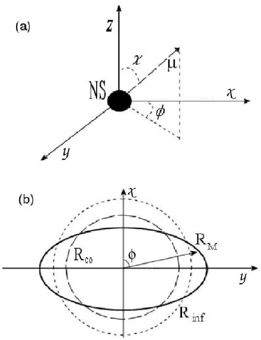
Figure 1: Schematic illustration of the NS-disk system for an oblique rotator. Figure (a) shows the relative positions of the magnetic dipole moment axis, the phase angle $\phi$, and the inclination angle $\chi$. The NS is assumed to rotate around the z-axis. Figure (b) is a two dimensional rapresentation of the position of the magnetosphere (continuous line) with respect to the corotation radius (long dashed line) and the infinity radius (short dashed line), for arbitrarily fixed values of the NS parameters.

2 Model description

2.1 Magnetosphere-disk interaction in an oblique rotator

In this section we discuss the main concepts and assumptions upon which our disk-magnetosphere model is based. The basic geometry is depicted in Figure 1. The axis of the magnetic moment $\mu$ of the neutron star (NS) is inclined with respect to the rotation axis by the magnetic colatitude $\chi$. In cylindrical coordinates $(r,\phi,z)$, where the z-axis coincides with the rotation axis, the component of the magnetic field in the disk plane is (Jetzer et al. 1998)

$$B^{2}=\frac{\mu^{2}}{r^{6}}\big{[}1+3(\sin{\chi}\sin{\phi})^{2}\big{]}\;,$$ (1)

under the assumption that the disk is planar and its axis is parallel to the spin axis of the NS. When the rotation axis of the NS is inclined (i.e. $\chi\neq 0$), the strength of the magnetic field in the plane of the disk depends on the longitude $\phi$. As shown below, this angular dependence results in an asymmetric magnetospheric boundary.

The fate of the matter funnelled from the accretion disk to the rotating, magnetized neutron star depends on a number of factors, the most important of which are the relative strength of the magnetic pressure and the pressure of the accreting material, and the relative velocity of the magnetosphere of the star at the inner radius of the disk with respect to the Keplerian velocity at that same radius. Following Lamb & Pethick (1974), the former condition can be formalized by equating the magnetic energy with the kinetic energy of the infalling matter:

$$\frac{1}{2}\rho v^{2}=\frac{B^{2}}{8\pi}\;.$$ (2)

In the free-fall approssimation the density is given by $\rho=\rho_{ff}=\dot{M}/(4\pi v_{ff}r^{2})$, where $v_{ff}=(2GM/r)^{1/2}$ is the free-fall velocity. Using these expressions, together with Eq.(1) and (2), the magnetospheric radius for an oblique rotator can be obtained (Jetzer et al. 1998; see also Campana et al. 2001):

$$R_{M}(\phi)=3.2\times 10^{8}\mu_{30}^{4/7}M_{1}^{-1/7}\dot{M}_{17}^{-2/7}\left[1+3(\sin{\chi}\sin{\phi})^{2}\right]^{2/7}\;,$$ (3)

where $\mu_{30}$ is the magnetic moment in units of $10^{30}$ G cm³, $M_{1}$ is the NS mass in units of $1~{}M_{\odot}$ and $\dot{M}_{17}$ is the accretion rate in units of $10^{17}$ g s^-1. The minimum radius $R_{\rm M}(0)$ also corresponds to $\chi=0$, the approximation usually adopted in models of the disk-magnetosphere interaction. The maximum radius $R_{\rm M}(\pi/2)$ is only a factor of $(1+3\sin^{2}\chi)^{2/7}\leq 1.49$ larger. Note that the elongated shape of the magnetospheric boundary plays a fundamental role in our model.

An important assumption of our model is that, during the rotation of the magnetosphere (whose shape depends upon the instantaneous position of the magnetospheric radius as a function of $\phi$), matter in the Keplerian disk is able to fill the region that separates the disk and the magnetospheric flow on a timescale shorter than the spin period of the star. This ensures that the inner boundary of the disk remains in constant contact with the magnetosphere. We show in the appendix that the Kelvin-Helmholtz instability operates on a sufficiently short timescale and wide range of radii that this assumption can be justified.

Accretion to the star is possible only under the condition that, at the magnetospheric radius, the Keplerian velocity of the accreting gas, $\Omega_{\rm K}(R_{M})$, is larger than the velocity $\Omega_{0}$ of the rotating magnetosphere of the star (equal to the velocity of the star), otherwise centrifugal forces will inhibit accretion (Illianorov & Sunyaev 1979). The above condition is equivalent to saying that the magnetospheric radius must be smaller than the corotation radius, $R_{\rm co}=(GM/\Omega_{0}^{2})^{1/3}$, which is the radius at which the Keplerian frequency of the orbiting matter is equal to the NS spin frequency $\Omega_{0}$. In an oblique rotator, the onset of the propeller stage will occur when $R_{M}(\phi)=R_{\rm co}$ at least in one point of the magnetospheric boundary. Note that, while a parallel rotator can be either in the propeller or in the accreting regime, an oblique rotator can be in both states simultaneously for different longitudes of the magnetospheric boundary. Indeed, this special feature of the oblique rotator was used by Campana et al. (2001) in building up a model that explained the dramatic luminosity variations seen in the BeppoSAX observation of the transient X-ray pulsar 4U 0115+63.

The interaction between the magnetosphere of the NS and the matter in the disk is likely to be at least partially anelastic because of dissipative effects in the mixing process between the magnetospheric plasma and the disk matter during the propeller phase. For clarity of presentation, here we consider first the two limiting cases of a completely anelastic and a completely elastic interaction, and then we will generalize our results to the partially anelastic case.

In the anelastic case, the magnetic field of the NS is able to force matter to corotate at the same velocity of the star, and it is endowed at the magnetospheric boundary with specific kinetic energy $\epsilon=1/2\Omega^{2}_{0}R_{M}^{2}$ and angular momentum $l=\Omega_{0}R_{M}^{2}$. In order for matter to be ejected from the system via the propeller mechanism, the magnetic field must provide it with enough energy to reach a velocity in excess of the local escape velocity at $R_{M}$. Because in the anelastic case the ejection velocity is $v_{ej}=\Omega_{0}R_{M}$, the requirement above converts to an ”ejection radius”

$$R_{\rm inf,ane}=(2GM/\Omega_{0}^{2})^{1/3}\simeq 1.26R_{\rm co}\;.$$ (4)

Only matter which is located beyond this radius during the interaction with the magnetosphere of the NS can be unbound from the system through the propeller mechanism. Therefore there exists a region ($R_{\rm co}<R_{M}<R_{\rm inf}$) in which the propeller is active but matter cannot be unbound from the sytem by merging with the disk matter (Spruit & Taam, 1993). We assume that matter in this zone is swung out and circularizes at the radius where its angular momentum equals the Keplerian value, i.e. when $l=\Omega_{0}R_{M}^{2}=l_{\rm K}=\Omega_{\rm K}(R_{\rm K})R_{\rm K}^{2}$ (here $R_{\rm K}$ is the circularization radius). This condition defines the Keplerian circularization radius:

$$R_{\rm K,{ane}}=\frac{\Omega_{0}^{2}R_{M}^{4}}{GM}\;.$$ (5)

Matter that is not ejected from the system will fall back into the disk and restart its motion toward the NS from the radius defined in Equation (5).

In the case of the elastic propeller, we assume that material in the disk at $R_{M}$ moves toward the magnetosphere with a tangential relative velocity of $-v_{\rm rel}=R_{M}(\Omega_{0}-\Omega_{\rm K})$, where $\Omega_{\rm K}$ is the Keplerian angular velocity at $R_{M}$. In a completely elastic interaction this matter bounces off at the magnetospheric boundary with an opposite velocity of $+v_{\rm rel}$ that in the non-rotating frame sums with $v_{\rm rot}=\Omega_{0}R_{M}$. Thus the ejection velocity is $v_{ej}=R_{M}[2\Omega_{0}-\Omega_{\rm K}(R_{M})]$. In this case the requirement that this velocity be larger than $v_{esc}(R_{M})$ can be written as:

$$\frac{R_{M}^{2}}{2}\Big{[}4\frac{GM}{R_{\rm co}^{3}}+\frac{GM}{R_{M}^{3}}-4\frac{GM}{R_{\rm co}^{3/2}R_{M}^{3/2}}\Big{]}\geq\frac{GM}{R_{M}}$$

where we have used the definition of the corotation radius. This equation can be solved as a function of the magnetospheric radius to define the limit beyond which ejection of matter to infinity is possible in the purely elastic case:

$$R_{\rm inf,{el}}=\Big{[}\frac{1+\sqrt{2}}{2}\Big{]}^{2/3}R_{\rm co}\simeq 1.13R_{\rm co}\;.$$ (6)

The matter leaving the magnetospheric boundary is endowed with specific angular momentum $l_{el}=R_{M}^{2}(2\Omega_{0}-\Omega_{\rm K})$; equating this to $l_{\rm K}$ gives a new circularization radius for matter that is not ejected to infinity. Using the same notation as above we find:

$$R_{\rm k,{el}}=\frac{R_{M}^{4}(2\Omega_{0}-\Omega_{\rm K})^{2}}{GM}\;.$$ (7)

Let us now consider the most general case of a partially elastic interaction. Following the formalism developed by Eksi et al. (2005), we define the “elasticity parameter” $\beta$, which is a measure of how efficiently the kinetic energy of the neutron star is converted into kinetic energy of ejected matter through the magnetosphere-disk interaction. Taking into account the definitions given above, we now consider the generalized rotational velocity of matter at the magnetospheric boundary:

$$v_{\rm gen}=\Omega_{\rm K}(R_{M})R_{M}(1-\gamma)$$ (8)

where $\gamma=(1+\beta)(1-\Omega_{0}/\Omega_{\rm K})$. The elastic case is obtained in the limit $\beta=1$, and the totally anelastic one when $\beta=0$. Using Equation (8) we can then generalize also the expression for the infinity radius

$$R_{\rm inf}=\Big{(}\frac{\beta+\sqrt{2}}{1+\beta}\Big{)}^{2/3}R_{\rm co}$$ (9)

and for the circularization radius

$$R_{\rm K}=R_{M}(1-\gamma)^{2}\;.$$ (10)

In our model we will consider the general case of a partially elastic interaction, and use $\beta$ as one of the model parameters.

Figure 1 (b) shows the various characteristic radii defined above on the disk plane $z=0$. Depending on the phase ($\phi$) and the inclination angle ($\chi$), it is possible to have regions of the magnetospheric boundary in which accretion is possible ($R_{M}(\phi,\chi)<R_{\rm co}$) together with other portions in which the propeller is already active, resulting in ejection of matter to larger radii ($R_{\rm co}<R_{M}(\phi,\chi)<R_{\rm inf}$), or to infinity ($R_{M}>R_{\rm inf}$). In those cases in which the inclination angle is sufficiently large, it is possible to have all the three regimes described above simultaneously.

It should be noted that, in our model, we consider ejection of matter from regions of the disk that are away from the corotation radius, where the Keplerian velocity of matter becomes rapidly supersonic (e.g. Frank, King, Raine 2003). This could in principle lead to the formation of supersonic shocks which can heat the plasma and eventually stop the ejection mechanism. However in this situation, due to the high relative rotation rate between the plasma inside the magnetosphere and that inside the disk, the Kelvin-Helmholtz instability can be very efficient. As previously discussed, this instability can lead to a large mixing of the two fluids, providing a mechanism to mantain the interaction between the magnetic field of the NS and the matter in the disk. Under these circumstances, it has been shown that outflowing bubbles of matter are likely to be accelerated magnetically by the NS towards the outer region of the disk (Wang & Robertson 1985), in turn supporting the idea that ejection far away from the corotation radius can be sustained.

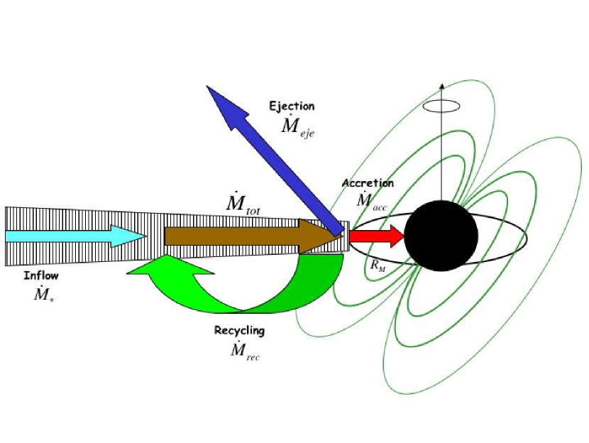
Figure 2: The fate of the matter provided by the companion at a rate $\dot{M}_{*}$ depends on the relative position of the magnetospheric radius with respect to the corotation radius and the ejection radius. Matter can be accreted, ejected or recycled into the disk.

2.2 Conditions for the existence of a limit cycle

Let $\dot{M}_{*}$ be the rate of inflowing matter, regulated through the Roche Lobe overflow or capture of part of the wind of the companion star. We assume that this matter possesses in all cases enough angular momentum that a prograde accretion disk forms. We further assume that the mass inflow at the inner disk boundary is azimuthally symmetric (i.e. independent of $\phi$). As illustrated in Figure 1 and discussed in §2.1, for a general, oblique, orientation of the magnetic field of the NS with respect to the normal to the disk and the spin axis of the NS (which we assume are parallel), there will be regions where $R_{M}(\phi)<R_{\rm co}$, and therefore some matter is able to accrete, regions for which $R_{M}(\phi)>R_{\rm inf}$ that result in matter being ejected, and intermediate zones with $R_{\rm co}<R_{M}(\phi)<R_{\rm inf}$ from which matter gets “recycled”. The fraction of material in each of these regions is expected to be proportional to the angle $\phi$ subtended by the relevant region in the magnetosphere as shown in Figure 1. As in §1, let us define $\dot{M}_{\rm acc}$, $\dot{M}_{\rm eje}$ and $\dot{M}_{\rm rec}$ to be respectively the rates of accreting, ejected and recycled material at any given time. These various components are illustrated in Figure 2. If $d\dot{M}_{\rm tot}/d\phi$ is the total rate of matter exchanged at the magnetosphere-disk boundary per unit angle, these components are given by $\dot{M}_{\rm comp}=1/2\pi\int_{\phi_{1}}^{\phi_{2}}d\phi\left(d\,\dot{M}_{\rm tot}/d\phi\right)$, where the integration interval $[\phi_{1},\phi_{2}]$ of $\phi$ is such that $R_{M}(\phi)<R_{\rm co}$ when comp=”acc” , $R_{\rm co}<R_{M}(\phi)<R_{\rm inf}$ when comp=”rec” and $R_{M}(\phi)>R_{\rm inf}$ when comp=”eje”. Figure 3 shows an example of these components as a function of the total mass inflow across the entire magnetospheric boundary, $\dot{M}_{\rm tot}$. At low values of $\dot{M}_{\rm tot}$, $R_{\rm inf}>R_{M}$ for all values of $\phi$, and therefore all matter is ejected (i.e. $\dot{M}_{\rm eje}=\dot{M}_{\rm tot}$). On the other hand, at high values of $\dot{M}_{\rm tot}$, $R_{\rm co}>R_{M}$ for any $\phi$, and therefore all matter is accreted ($\dot{M}_{\rm acc}=\dot{M}_{\rm tot}$). For values of $\dot{M}_{\rm tot}$ such that $R_{M}(\phi)$ crosses $R_{\rm co}$ at some values of $\phi$, $\dot{M}_{\rm rec}\neq 0$.

Figure 3: The various contributions to the total accretion rate $\dot{M}_{\rm tot}=\dot{M}_{\rm acc}+\dot{M}_{\rm rec}+\dot{M}_{\rm eje}$ at the magnetospheric-disk boundary. The system parameters are $B=6\times 10^{13}$ G, $\nu=9$ mHz, $\chi=45^{\circ}$, $\beta=0.3$.

While the total mass inflow rate available to the system is determined by the mass transfer rate from the companion, $\dot{M}_{*}$, the value of the magnetospheric radius $R_{M}$, on the other hand, is determined by the total pressure of the accreting matter, i.e. $\dot{M}_{\rm tot}=\dot{M}_{\rm acc}+\dot{M}_{\rm eje}+\dot{M}_{\rm rec}$. Since, in general, $\dot{M}_{\rm tot}\geq\dot{M}_{*}$, the magnetospheric radius can be smaller than it would be if the “recycled” mass component were not accounted for (as commonly assumed in the literature). Therefore, including $\dot{M}_{\rm rec}$ in the computation of $R_{M}$, allows accretion at the same rate to occur for smaller values of $\dot{M}_{*}$ than it would otherwise.

In order to demonstrate the existence of a limit cycle, testified by a hysteresis-like loop in the $\dot{M}_{*}-\dot{M}_{\rm tot}$ plane, we start by noting that the rate at which matter is “recycled”, $\dot{M}_{\rm rec}$, does not contribute to the mass budget; therefore a steady-state solution is possible only if

$$\dot{M}_{*}=\dot{M}_{\rm acc}+\dot{M}_{\rm eje}\;.$$ (11)

Let us therefore examine the behaviour of the curve $\dot{M}_{\rm tot}$ as a function of the accretion rate $\dot{M}_{\rm acc}+\dot{M}_{\rm eje}=\dot{M}_{*}$. An example of such a curve for a rotator inclined by an angle of $\chi=50^{\circ}$ is shown in Figure 4. All the characteristic parameters of the NS ($B$, $\Omega_{0}$, $R_{NS}$, $M_{NS}$) and the angle $\chi$ are kept fixed while the mass supply from the companion is varied. For a given value of the external rate of mass supply $\dot{M}_{*}$, the corresponding points on the curve yield the value (or values) of $\dot{M}_{\rm tot}$ for which there exists a solution. Again, we stress that the “state” of the system, and the characteristics of the solution, are determined by $\dot{M}_{\rm tot}$ since it is this quantity (and not $\dot{M}_{*}$) which determines the position of $R_{M}$. There can be multiple solutions for a given $\dot{M}_{*}$, and the one that is realized at a certain time depends on the previous history of the system. This situation is reminiscent of a system with hysteresis, and in fact, as Figure 4 shows, the shape of the curve $\dot{M}_{\rm tot}(\dot{M}_{*})$ resembles a hysteresis curve, where the role of the external magnetic field is played by the rate of mass supply by the companion, $\dot{M}_{*}$ (the independent variable in the present context). If at a certain point the system is in, say, the state indicated by the point “C” in the figure, and $\dot{M}_{*}$ increases, the solution (i.e. only available state for the system) will be forced to jump to the state indicated by point “D”. As $\dot{M}_{*}$ decreases, the solution will move from “D” to “A” but from that point on, any further decrease in $\dot{M}_{*}$ will cause the solution to jump to point “B”. Therefore, like in the traditional hysteresis cycle, continuous variations in $\dot{M}_{*}$ result in discontinuous states for the system.

In the following section, after discussing the computation of the torque, it will be shown that the points where the solution jumps from one place to another in the $\dot{M}_{\rm tot}(\dot{M}_{*})$ curve often straddle the point of torque reversal. Therefore, transitions between different states are often characterized by a torque reversal.

The case we have illustrated in Figure 4 is only an example of a cyclic behaviour. The shape of the curve $\dot{M}_{\rm tot}(\dot{M}_{*})$ changes with the parameters $\chi$ and $\beta$ (while $\nu$ and $B$ only cause a translation in the $\dot{M}_{\rm tot}-\dot{M}_{*}$ plane). This can result in several types of cycles with a different number of jumps. More examples are shown in Figure 5.

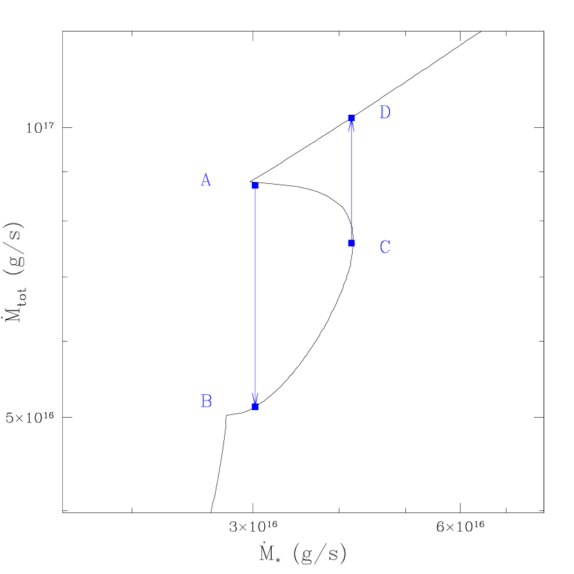
Figure 4: Schematic representation of the hysteresis-type limit cycle. The arrows indicate the points where the system ”jumps” between different states as a result of variations in the external mass supply rate $\dot{M}_{*}$. The system parameters in this example are $\nu=9$ mHz, $B=6\times 10^{13}$ G, $\chi=80^{\circ}$, $\beta=0$.

2.3 Torque and luminosity in the different states of an oblique rotator

We calculate here the net specific angular momentum trasferred between the disk and the NS. In the region of the magnetospheric boundary where accretion is allowed, the net specific angular moment transferred from the disk to the NS is given by

$$l_{\rm acc}=\frac{1}{2\pi}\int_{R_{M}<R_{\rm co}}(GMR_{M})^{1/2}d\phi\;.$$ (12)

In the ejection region, the NS accelerates the material to the ejection velocity, which, as discussed in §2.1, is different in the two limiting cases of a completely elastic or anelastic propeller. For the general case of a partially elastic interaction, using Equation (8), the angular momentum given by the NS to the ejected matter is:

$$l_{eje}=\frac{1}{2\pi}\int_{R_{M}>R_{\rm co}}(v_{gen}R_{M}-\Omega_{\rm K}R_{M}^{2})d\phi={}$$ (13)

$${}\frac{1}{2\pi}\int_{R_{M}>R_{\rm co}}\Omega_{\rm K}R_{M}^{2}(1+\beta)(\Omega_{0}/\Omega_{\rm K}-1)d\phi\;.$$

By relating this transfer of angular momentum between the NS and the disk to the variation of the NS angular momentum, we have

$$\frac{d\Omega_{0}}{dt}=\frac{\dot{M}_{\rm tot}l_{\rm tot}}{I}$$ (14)

where $l_{\rm tot}$ is the sum of the angular momentum computed from Equations (12) and (13), and we have assumed that the variation of the NS moment of inertia ($I$) is negligible. Using equations (12) and (13) in (14), we obtain:

$$\frac{d\Omega_{0}}{dt}=\frac{\dot{M}_{\rm tot}}{2\pi}\int_{0}^{2\pi}(GMR_{M})^{1/2}\big{\{}1-\theta(R_{M}-R_{\rm co})\big{[}(1+\beta)(\Omega_{0}/\Omega_{\rm K}-1)\big{]}\big{\}}d\phi$$ (15)

where $\theta(R_{M}-R_{\rm co})$ is $1$ for $R_{M}>R_{\rm co}$ and $0$ for $R_{M}<R_{\rm co}$.

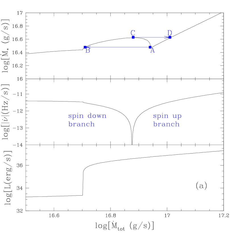
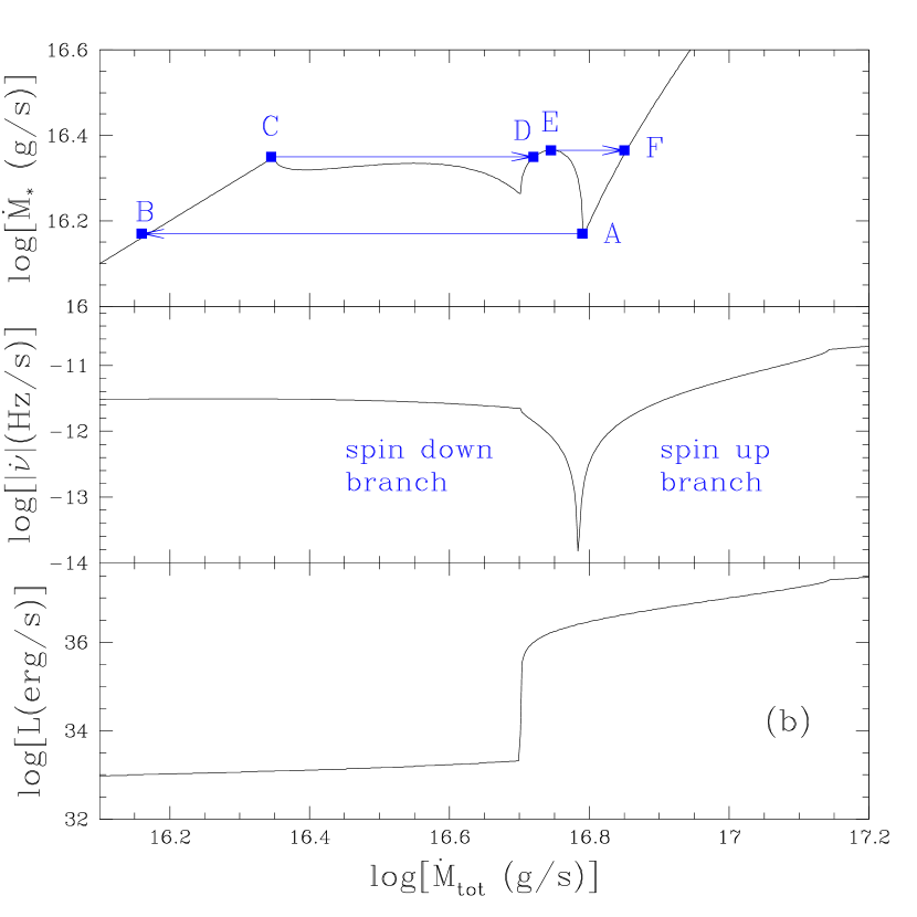
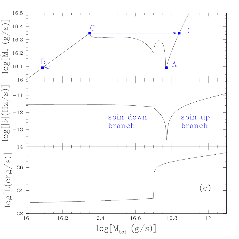
Figure 5: Various types of hysteresis limit cycles. The system parameters are $\nu=9$ mHz, $B=6\times 10^{13}$ G and $\beta=0$ in all cases, while $\chi=80^{\circ}$ in panel (a), $\chi=50^{\circ}$ in panel (b) and $\chi=47^{\circ}$ in panel (c). In the top panels of each case, the arrows indicate the points where the system ”jumps” between different states as a result of variations in the external mass supply rate $\dot{M}_{*}$. The middle panels show that, under most circumstances, a jump is accompanied by a torque reversal and, in some cases, by an abrupt change in luminosity (displayed in the bottom panels).

Next we compute the different contributions to the luminosity. A schematic representation of these contributions is shown in Figure 7. Let us consider first the region of the magnetosphere in which there is accretion ($R_{M}(\phi)<R_{\rm co}$). The accretion luminosity is given by the potential and kinetic energy released by matter falling from the magnetospheric radius to the surface of the neutron star; this is

$$L_{\rm acc}=\int_{R_{M}<R_{\rm co}}\left[GM\left(\frac{1}{R_{NS}}-\frac{1}{R_{M}}\right)+\frac{1}{2}\Omega^{2}\left(R_{M}^{2}-R_{NS}^{2}\right)\right]d\dot{M}_{\rm acc}\;,$$ (16)

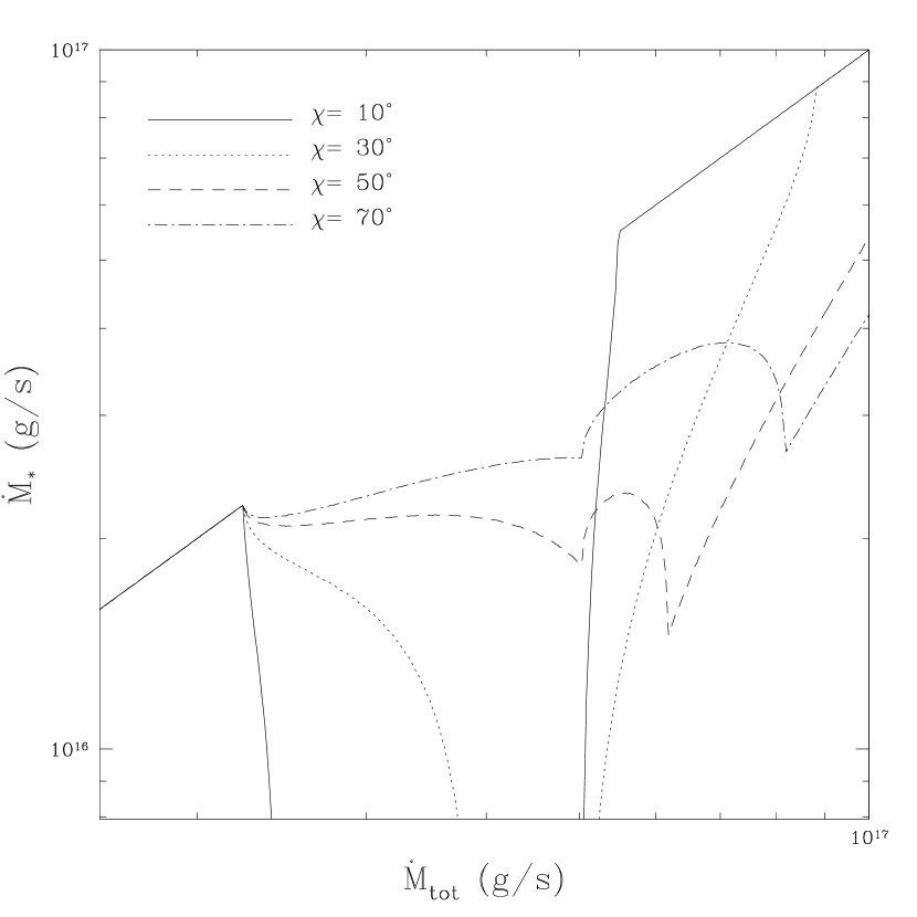
Figure 6: The break of the cyclic solution in the $\dot{M}_{*}-\dot{M}_{\rm tot}$ plane is shown for a system with $\nu=9$ mHz s, $B=6\times 10^{13}$ G, $\beta=0$ (left panel) and $\beta=1$ (right panel). When the inclination angle is small, it is no longer possible to find a steady state, cyclic solution. The value of $\chi$ around which the solution breaks depends on the anelasticity parameter $\beta$ but is independent of the values of $\nu$ and $B$.

where $\dot{M}_{\rm acc}$ is the fraction of $\dot{M}_{\rm tot}$ which accretes. Next we consider the contribution to the luminosity coming from the ”recycled matter”. This can be calculated by summing the luminosity derived from the release of energy of matter impacting the disk at $R_{\rm K}$, and the luminosity released from the same matter spiralling in the disk from $R_{\rm K}$ back to $R_{M}$. This gives

$$L_{\rm rec}=\int_{R_{\rm co}<R_{M}<R_{\rm inf}}\left(\frac{v_{gen}^{2}}{2}-\frac{GM}{2R_{M}}\right)d\dot{M}_{\rm rec}$$ (17)

where $\dot{M}_{\rm rec}$ is the rate corresponding to the ”recycling” part of the magnetospheric boundary ($R_{\rm co}<R_{M}(\phi)<R_{\rm inf}$).

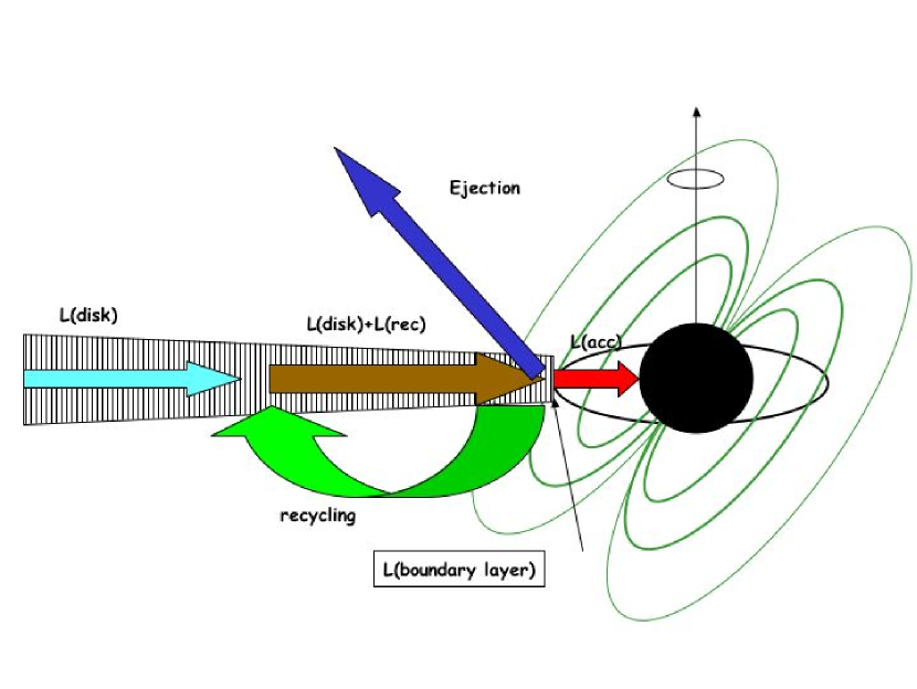
Figure 7: The various contributions to the total luminosity budget for an accreting neutron star.

Another contribution to the total luminosity is provided by the release of energy in the boundary layer which separates the magnetosphere from the Keplerian disk. This term applies to matter at any longitude $\phi$ if we consider a completely anelastic propeller ($\beta=0$), because in this case the magnetosphere forces matter to corotate with it during both the accretion and the propeller regime. On the other hand, in the limit of a completely elastic propeller ($\beta=1$), this term is present only for those angles $\phi$ for which $R_{M}<R_{\rm co}$ and matter is thus slowed down in the boundary layer before it can begin falling toward the NS. If we consider a generic value for the elasticity parameter, the luminosity of the boundary layer can be written as:

$$L_{\rm BL}=\left\{\begin{array}[]{ll}\displaystyle\frac{\dot{M}_{\rm tot}}{4\pi}\int_{0}^{2\pi}\big{[}R_{M}^{2}(\Omega_{\rm K}^{2}-\Omega_{0}^{2})\big{]}d\phi&{\rm for}\;\;R_{M}<R_{\rm co}\\ \displaystyle\frac{\dot{M}_{\rm tot}}{4\pi}(1-\beta)\int_{0}^{2\pi}\big{[}R_{M}^{2}(\Omega_{0}^{2}-\Omega_{\rm K}^{2})\big{]}d\phi&{\rm for}\;\;R_{M}\geq R_{\rm co}\;.\end{array}\right.$$ (18)

Finally, we have to account for the luminosity produced by the matter inflowing from the companion as it spirals in towards the magnetospheric radius in the Keplerian disk. This contribution, which is obviously present in all different regimes, is given by

$$L_{\rm disk}=\frac{GM\dot{M}_{*}}{2R_{M}}\;.$$ (19)

Figure 8: The various contributions to the total luminosity budget $L_{\rm tot}=L_{\rm acc}+L_{\rm rec}+L_{\rm disk}+L_{\rm BL}$ for an accreting neutron star as function of the mass accretion rate from the companion, $\dot{M}_{*}$. The system parameters are $\nu=9$ mHz, $B=6\times 10^{13}$ G, $\chi=80^{\circ}$ in the top panels and $\nu=9$ mHz, $B=10^{9}$ G, $\chi=80^{\circ}$, in the bottom ones. The two limiting cases of a completely elastic interaction (left panels) and of a completely anelastic interaction (right panels) are shown.

It is important to emphasize that in our model both the torque and the luminosity depend on the total mass inflow rate $\dot{M}_{\rm tot}$ at the magnetospheric boundary, and this can take different values for the same mass accretion rate $\dot{M}_{*}$. The three panels of Figure 5 show the behaviour of the torque and luminosity as a function of $\dot{M}_{\rm tot}$ for three combinations of NS parameters. These are chosen to represent different types of limit cycles (also shown in the figure for each case – note the axes here are swapped with respect to Figure 4 for consistency with the other panels). In Figure 5(a), a transition between the points A and B is accompanied by a reversal from spin up to spin down, while the jump from point C to D will cause a transition from spin down to spin up. The luminosity is at its lowest at point B and at its highest at point D, but the overall variation during the cycle is well within an order of magnitude. A more complicated cycle is depicted in Figure 5(b); here a transition from point A to B causes a spin-up to spin-down reversal, while the opposite happens during the jump from point E to F. This cycle comprises also another jump, from point C to D, with both points on the spin-down branch. The luminosity varies by more than three orders of magnitude during the cycle, being at its lowest during most of the spin down phase. The third example of limit cycle, the one shown in Figure 5(c), has only two allowed jumps, both of them straddling the point of torque reversal, as in case a), but the luminosity is substantially larger when the system is on the spin-up branch (A – D), than when it is on the spin-down branch (B – C).

Whether there exists a limit cycle depends crucially on the angle $\chi$: this has to be large enough to ensure that some regions of the magnetosphere are in the accretion regime while, at the same time, others are in the propeller phase. There exists a critical value of the magnetic colatitude, $\chi_{\rm crit}$, below which the steady state solution breaks into two disjoint curves and it is no longer possible to find a cyclic behaviour through a sequence of steady-state solutions. This is illustrated in Figure 6 for the cases $\beta=0$ and $\beta=1$. If the accretion rate $\dot{M}_{*}$ from the companion is above a certain value (which depends on $\nu$, $B$, $\chi$ and $\beta$), only one solution is available to the system, and it corresponds to the spin up branch (see Figure 5). On the other hand, if $\dot{M}_{*}\lesssim\dot{M}_{\rm crit}$ (for the example under consideration, $\dot{M}_{\rm crit}=2.4\times 10^{16}$ g/s for $\beta=0$ and $\dot{M}_{\rm crit}=3.5\times 10^{16}$ g/s for $\beta=0$, but it varies with $\nu$ and $B$), then multiple solutions are available for any value of $\chi$ displayed, and the one that is realized at any given time depends on the history of the system. However, a cyclic jump of the solutions between the spin-up and the spin-down branches can only be realized for angles above $\chi_{\rm crit}$.

The critical angle ranges from about $25^{\circ}-30^{\circ}$ for $\beta=1$ to about $40^{\circ}-45^{\circ}$ for $\beta=0$, and, for a given $\beta$, it is independent of $\nu$ and $B$. Therefore, for the curves shown in the figure, a limit cycle can only be achieved in the cases with $\chi=30^{\circ}$ and $\chi=40^{\circ}$ for $\beta=1$, and in the cases with $\chi=50^{\circ}$ and $\chi=70^{\circ}$ for $\beta=0$. In the other cases displayed, the $\dot{M}_{*}(\dot{M}_{\rm tot})$ curve is discontinuous. The shape of the curve is such that, if the system is spinning up, a solution on the spin-up branch can be found for any value of $\dot{M}_{*}$, and therefore the system will continue spinning up. On the other hand, if the system is originally on the spin-down branch (which is possible only for $\dot{M}_{*}\lesssim\dot{M}_{\rm crit}$), then any decrease in $\dot{M}_{*}$ will keep the system on the spin-down branch, while an increase in $\dot{M}_{*}$ above $\dot{M}_{\rm crit}$ will cause a jump on the spin-up branch, and from that point on the system will be spinning up independent of the value of $\dot{M}_{*}$. Note that, depending on the angle $\chi$, there can be spin-up solutions even at very low mass inflow rates $\dot{M}_{*}$. This result is a novelty of our model, deriving from the fact that the recycled mass component $\dot{M}_{\rm rec}$ can keep the magnetospheric radius in “pressure” even if $\dot{M}_{*}$ is very small.

Among all the components that make up the total luminosity, the accretion term is the only that is certainly pulsed, since the accretion material is funnelled by the magnetic field of the star onto the NS magnetic poles, where its energy is released. The accretion luminosity therefore varies with the phase of the star, resulting in a pulsating flux. Also the boundary layer luminosity might be pulsed at the NS spin. Therefore, the maximum pulsed fraction in our model is constrained to be between $f_{\rm pul}=L_{\rm acc}/L_{\rm tot}$ and $f_{\rm puls}=(L_{\rm acc}+L_{\rm BL})/L_{\rm tot}$.

Note that the sum of the various contributions in Equations (16), (17), (18), (19) can result in a complex, non-monotonic dependence of $L_{\rm tot}$ as function of the accretion rate from the companion, $\dot{M}_{*}$. In the classical model of accretion onto magnetized neutron stars, the transition between the standard accretion regime onto the NS surface to the regime of accretion onto the magnetospheric boundary in the propeller regime is marked by the change between the $\propto\dot{M}_{*}$ and the $\propto\dot{M}_{*}^{9/7}$ scaling of the luminosity (Stella et al. 1994; Campana & Stella 2000). In the propeller phase, the underlying assumption of these works is that the main contribution to the luminosity derives from the disk luminosity (Eq. 19). In the present model, this might not be the case if there is a non-negligible contribution to the luminosity from recycled matter. Moreover, at low accretion rates, we find that the contribution to the luminosity from the boundary layer generally dominates over that from the disk for an anelastic propeller (see Figure 8). For sufficiently low values of $\dot{M}_{*}$ (so that $\Omega_{\rm K}^{2}(R_{M})/\Omega_{0}^{2}\ll 1$), the boundary layer luminosity scales as $\propto\dot{M}_{*}^{3/7}$, while $L_{\rm BL}\propto\dot{M}_{*}^{9/7}$ at high values of $\dot{M}_{*}$ (for which $\Omega_{\rm K}^{2}(R_{M})/\Omega_{0}^{2}\gg 1$). When the corotation radius is of the order of the magnetospheric radius, however, these dependences are changed. Since the Keplerian frequency at the magnetospheric radius is an increasing function of $\dot{M}_{*}$, in the propeller regime the term $\left|\Omega_{0}^{2}-\Omega_{\rm K}^{2}(R_{M})\right|$ decreases with the increase of $\dot{M}_{*}$, while in the accretion regime the same term increases with increasing $\dot{M}_{*}$. As a result, when $R_{M}$ is of the order of $R_{\rm co}$, the luminosity of the boundary layer has a flatter dependence on $\dot{M}_{*}$ for $R_{M}>R_{\rm co}$ and a steeper dependence for $R_{M}<R_{\rm co}$. This can be seen in Figure 8. Both the case of a completely anelastic propeller ($\beta=0$), and a totally elastic one ($\beta=1$) are considered, showing respectively the maximum and the minimum boundary layer luminosity that the system can have. In the former case we find that, for sufficiently low accretion rates (so that the whole magnetospheric boundary is in the propeller regime), the boundary layer luminosity is substantially larger than the disk luminosity. The relative contribution $L_{\rm BL}/L_{\rm disk}$ clearly increases as the degree of anelasticity increases, since $L_{\rm BL}\propto(1-\beta)$. As the mass accretion rate $\dot{M}_{*}$ increases, so that at least some regions of the magnetospheric boundary are in the accretion regime, the disk luminosity begins to dominate over that of the boundary layer (this is now independent of $\beta$). However, $L_{\rm BL}$ has a stronger dependence on $\dot{M}_{*}$, and, for sufficiently large $\dot{M}_{*}$ that $R_{M}\ll R_{\rm co}$, $L_{\rm BL}$ becomes $\sim L_{\rm disk}$.

The two panels in Figure 8 show the cases of a slow pulsar ($\nu=9$ mHz) and a fast one ($\nu=100$ mHz). The discussion above regarding the relative contribution of $L_{\rm BL}$ and $L_{\rm disk}$ to the total luminosity budget holds in both cases. Furthermore, once accretion sets in, the accretion luminosity dominates over both $L_{\rm disk}$ and $L_{\rm BL}$. The slower the pulsar, the larger is this term compared to the others. Therefore, in the accretion regime and for $R_{M}\ll R_{\rm co}$, $L_{\rm tot}\propto\dot{M}_{*}$ as in the classical models. However, for $R_{M}\sim R_{\rm co}$, the presence of the “recycled” term of luminosity in our model causes a non-monotonic dependence of the total luminosity on $\dot{M}_{*}$, with multiple solutions allowed. The actual solution that is realized at any given time will depend on the history, i.e. whether the system is on the spin-up or spin-down branch of the limit cycle (see Figure 4). This is an important difference of our model with respect to the classical solution where, once the system is in the accreting phase, the luminosity scales monotonically with $\dot{M}_{*}$. On the other hand, Figure 8 shows that there are regions for which a small variation in $\dot{M}_{*}$ can cause a large jump in luminosity.

Similar to the luminosity, the behaviour of the torque in the surroundings of the region with $R_{M}\sim R_{\rm co}$ is complex and non-monotonic. Small variations in $\dot{M}$ can cause the system to jump between states with opposite sign of the torque. Within this region, because of the complex dependence of both $L$ and $\dot{\Omega}$ on $\dot{M}_{*}$, our model does not make any specific prediction regarding correlations between torque and luminosity. In most situations, these are expected to be uncorrelated, and different types of limit cycles (see Figure 5) will generally lead to different behaviours in the various spin-up and spin-down phases.

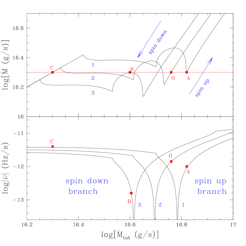
Figure 9: Variation of the function $\dot{M}(\dot{M}_{\rm tot})\equiv\dot{M}_{\rm acc}+\dot{M}_{\rm eje}$ (top panel) and of the corresponding spin rate variation (bottom panel) at three different times during a spin up/spin-down cycle. The system parameters are $B=6\times 10^{13}$ G, $\chi=45^{\circ}$ and $\beta=0.3$. The three curves correspond to frequencies $\nu=9.1$ mHz (curve 1), $\nu=8.3$ mHz (curve 2) and $\nu=7.7$ mHz (curve 3). Allowed states for the system are only those satisfying the condition $\dot{M}_{*}=\dot{M}(\dot{M}_{\rm tot})$; in this case, $\log(\dot{M}_{*})=16.3$. When multiple solutions are allowed, the state in which the system will be found depends on its previous history.

2.4 Cyclic spin-up/spin-down evolution at a constant $\dot{M}_{*}$

In systems in which mass transfer takes place through Roche Lobe overflow, the rate at which material is fed to the disk is expected to be roughly constant, or characterized by relatively low-amplitude, long-term variations. We are not concerned in this section with the accretion disk instabilities that likely give rise to the very large amplitude variations of the mass inflow rate in binary X-ray transient systems. Rather, in the following we describe how recurrent episodes of spin up and spin down can be achieved in our model in response to a strictly constant accretion rate $\dot{M}_{*}$ from the companion star.

Figure 9 shows the behaviour of the curve $\dot{M}=\dot{M}_{\rm eje}+\dot{M}_{\rm acc}$ (top panel) and the corresponding frequency derivative, $\dot{\nu}$, (bottom panel) as a function of $\dot{M}_{\rm tot}$ and for different values of the period (corresponding to different times). The parameters $B$, $\chi$ and $\beta$ are the same in all cases. They yield a limit cycle of the type described in Figure 5(b). While the specific points of torque reversal will vary depending on the type of cycle (as shown in the various examples of Figure 5), the underlying structure determining the transitions is the same in all cases and therefore we analyze in detail only one of the possible scenarios.

In order to illustrate how the spin up/spin down states are achieved at a constant $\dot{M}_{*}$, let’s start, say, with the system at a frequency $\nu$ so that the corresponding $\dot{M}(\dot{M}_{\rm tot})$ curve is the one labeled “2” in Figure 9, and let’s assume that the system is in a spin-up state. The intersection between the curves $\dot{M}$ and $\dot{M_{*}}$ on the spin-up branch of the cuspid determines the value of $\dot{M}_{\rm tot}$, $\dot{M}_{\rm tot,sol}$, corresponding to the allowed spin-up state for that value of the frequency. This value of $\dot{M}_{\rm tot,sol}$ in turn determines the value of the frequency derivative at that point in time (point “O” in both panels of the figure). The frequency at time $t+dt$ is simply determined as $\nu(t+dt)=\nu(t)+d\nu(\dot{M}_{\rm tot,sol})/dt$. As the pulsar spins up, the curve “2” moves towards curve “1” until the point at which the spin-up branch of the solution rises higher than the system $\dot{M}_{*}$ (point A). From that point on, the only possible state for the system that satisfies the condition $\dot{M}=\dot{M}_{*}$ is the one corresponding to point C in the figure, on the spin-down branch (negative torque). Once again, the new (current) value of $\dot{M}_{\rm tot,sol}$ determines the actual value of $\dot{\nu}$ (corresponding point C in bottom panel) which is used for the next time step to determine the new $\nu$. While on the spin down branch of the solution, the curve $\dot{M}$ now moves from the curve “1” towards the curve “2” and then “3”. Spin down continues until this branch of the solution does not intersect any longer the $\dot{M}_{*}$ line (point B), at which point the only allowed state for the system to be is on the spin-up branch, and the system reverses from spin down to spin up. This is the beginning of a new cycle.

Figure 10: An oblique NS rotator with magnetic field $B=6\times 10^{13}$ G, inclination angle $\chi=45$ deg, and elasticity parameter $\beta=0.3$ is able to reproduce the main spin-up/spin down characteristics of GX 1+4. The luminosity is comparable during the spin-up and spin-down phases, except for a few years at the beginning of the spin-down phase, when it drops abruptly.

In this model, the points of spin reversals are determined by the maximum and minimum of the $\dot{M}(\nu)$ curve. The shape of this curve depends on the anelastic parameter $\beta$ and on the angle $\chi$. For a given $\beta$ and $\chi$, a change in the strength of the magnetic field simply results in a shift of the curve without a change in shape: a higher $B$ field would move the curve to higher values of $\dot{M}_{\rm tot}$, therefore resulting in stronger spin-up and spin-down torques, and hence in a shorter timescale for torque reversals. For the model to work as described, it is clear that the points where the solution jumps must straddle the point of torque reversal. We find this to be the case for a wide range of combinations of $\chi$ and $\beta$. However, for each value of $\beta$, there is a narrow range of angles $\chi$ for which the torque inversion point falls outside the allowed region for the transitions. For these particular and rare cases, the system would tend towards the point $\dot{\Omega}_{0}=0$ and remain there, for a strictly constant $\dot{M}_{*}$. However, small fluctuations in $\dot{M}_{*}$ can still cause the system to jump from one solution to another. For the rest of this discussion we will focus on the greatest majority of cases for which torque reversals naturally occur at $\dot{M}_{*}$ = const, unless we explicitly state otherwise.

If the magnetic colatitude angle $\chi$ is larger than $\chi_{\rm crit}$, the system is bound to end up in a cyclic sequence of spin-up/spin-down transitions. In fact, as it can be seen from Figure 9, if the system starts with a much larger frequency than the maximum frequency in the cycle, $\nu_{\rm max}$, it will spin down since only one solution (on the spin down branch) is allowed as long as $\nu>\nu_{\rm max}$. Similarly, if the system starts with a frequency much smaller than the mimimum frequency in the cycle, $\nu_{\rm min}$, it will spin up as only one solution (on the spin up branch) is allowed as long as $\nu<\nu_{\rm min}$. Therefore, our model predicts that the system, independent of the initial conditions, eventually settles in a region where there are cyclic transitions between spin-up and spin-down states. This limit cycle is not induced by external perturbations, but is the natural equilibium state torwards which the system tends.

3 Application of our model to persistent X-ray pulsars

In the following, we will apply our model to two objects for which long term-monitoring showed a marked transition between a spin-up and spin-down phase. We will then discuss the way our model can be generalized to other cases where short-term episodes of spin-up/spin-down are superimposed onto longer term spin-up or spin-down trends. The most comphrensive monitoring of the spin behaviour of accreting X-ray pulsars in binaries is given in Bildsten et al. (1997), and here we briefly summarize the observations for the two cases that we model.

3.1 GX 1+4

GX 1+4, discovered in 1970 through an X-ray balloon experiment (Lewin, Ricker & McClintock 1971) is an accreting X-ray pulsar binary hosting an M red giant (Davidsen et al. 1977); the orbital period is likely to be of a few years (Chakrabarty & Roche 1997). Early observations through the 1970s showed that this source was spinning up at a very high pace with a spin-up timescale $|\nu/\dot{\nu}|\sim 40$ yr. The frequency changed from $\sim 7.5$ mHz to $\sim 9$ mHz during the first 15 years of observations. In the early 1980s, however, the flux dropped abruptly and the source could not be detected by Ginga. Given the sensitivity of the instrument, the flux must have decresead by more than two orders of magnitudes for a few years. Once its flux raised, the source could be monitored again, and it was found to spin down on a timescale comparable to the previous spin-up timescale (Makishima et al. 1988).

A solution that closely reproduces the observed source behaviour was found by running the time-dependent code described in §2.4 for a range of parameters $B,\chi,\beta$. The corresponding value of $M_{*}$ is determined so that the point of torque reversal of the system between spin up and spin down matches the observed value. The larger the magnetic field, the larger $\dot{M}_{*}$ and hence the torque, and therefore the more rapid the timescales of the torque transitions are; the parameters $\chi$ and $\beta$, by determining the shape of the $\dot{M}$ curve, especially influence the total frequency range $\nu_{\rm max}-\nu_{\rm min}$ that the system spans in a cycle.

For the case of GX 1+4, we found that a good choice of parameters is the combination $B=6\times 10^{13}$ G, $\chi=45^{\circ}$, and $\beta=0.3$. These yield a cycle of the type displayed in panel (b) of Figure 5 and in Figure 9. In particular, the parameters $B$, $\chi$ and $\beta$ used in Figure 9 are the same as those used for GX 1+4. The accretion rate provided by the donor companion must be $\dot{M}_{*}\sim 2\times 10^{16}$ g/s in order to produce a turnover in frequency around 9 mHz. With this choice of parameters, Figure 10 shows the behaviour of the system that our model predicts. Cycles of spin-up/spin-down alternate in response to torque reversals. The luminosity of the source is comparable during the spin-up and spin-down phases, except for a few years around the time of spin reversal from spin up to spin down, when it drops abruptly. This is due to the fact that, after the system has “jumped” to point “C” in Figure 9 (at the beginning of the spin down phase), there are no regions in the magnetosphere-disk boundary where accretion onto the NS can take place, the NS is in the propeller regime, and therefore $\dot{M}_{\rm acc}=0$ (see Figure 3). During that time, the only contribution to the luminosity comes from the disk and the boundary layer, which are however much smaller than the accretion luminosity (since this is a slow pulsar). A prediction of our model is that, while large drops in luminosity can be expected when the system reverses from spin up to spin down, they should not occur in correspondence of the spin-down/spin-up transition, because when this transition occurs (refer to the jump from point “B” to point “A” in Figure 9), most regions at the magnetospheric boundary are allowed to accrete. While these overall features are generally robust predictions of our model, the detailed variation of $\dot{M}$ (and hence the luminosity) with torque shown in our examples should not be taken too rigorously. These variations depend on the shape of the $\dot{M}(\dot{M}_{\rm tot})$ curve, and this is in turn determined by the shape of the magnetospheric boundary as a function of time. As discussed in §3.3, a number of effects neglected here can influence this shape, and hence affect the detailed behaviour of the solution. In particular, note that observations of GX 1+4 show that luminosity and torque strength are correlated during part of the spin down phase (Chakrabarty et al. 1997b). This feature is not reproduced by the current version of our model.

3.2 4U 1626-67

4U 1626-67, discovered by SAS-3 in 1977 (Rappaport et al. 1977) is an ultracompact binary with an extremely low-mass companion (Levine et al. 1988; Chakrabarty et al. 1997a) and a 42 minute orbital period (Middleditch et al. 1981). During the first $\sim 20$ years of observations, the source was found to spin up with a timescale $\nu/\dot{\nu}$ of about 5000 yr. The frequency increased from 130.2 mHz to about 130.5 mHz, at which point the source started to spin down. Unlike the case of GX 1+4, there was no evidence for a large change in the bolometric luminosity of the source during the transition.

Figure 11: An oblique NS rotator with magnetic field $B=2.5\times 10^{12}$ G, inclination angle $\chi=68^{\circ}$, and elasticity parameter $\beta=0$ is able to reproduce the main spin-up/spin down characteristics of 4U 1626.

The very long timescale for spin reversal of this source (due to a smaller torque compared to the case of GX 1+4) requires a smaller magnetic field. We found that our model yields a reasonable match to the observations with the choice of parameters $B=2.5\times 10^{12}$ G, $\chi=68^{\circ}$, $\beta=0$. The corresponding solution found with our model is displayed in Figure 11. The upper panel shows only one spin-up/spin-down torque reversal, since the complete spin-up/spin-down cycle, of the order of several thousand years, lasts much longer than the observed time. Although the luminosity somewhat drops around the time of spin reversal, it does so to a lesser extent and for a much shorter time than for the case of GX 1+4. The reason for these differences lies in the variation of the shape of the function $\dot{M}(\dot{M}_{\rm tot})$ for different choices of the parameters $\chi$ and $\beta$. The parameters that best match the solution for 4U 1626-67 yield a cycle of the type in panel (a) of Figure 5. The transition from spin up to spin down (point A to B in the figure) is accompanied by a less dramatic variation in luminosity than it is for the cycles of the type shown in panels (b) and (c). Note how, for this source, since the observation window is much smaller than the timescale for torque reversal, other torque inversions are not expected in the near future, unless induced by external perturbations.

3.3 Generalizations and limitations of our model

The two examples given above, for two sources spinning up and down at very different rates, show that our model can reproduce different types of cyclic behaviours. In the two cases discussed, we assumed that the mass accretion rate from the companion, $\dot{M}_{*}$, does not vary with time. Under this assumption, our model predicts that the points of torque reversals will always occur at the same value of the frequency. On the other hand, if the donor accretion rate varies with time, this will no longer be the case. If $\dot{M}_{*}$ increases with time, then the points of torque reversals will occur at larger frequencies as time goes on. Viceversa if $\dot{M}_{*}$ decreases with time, then the points of torque reversals will occur at smaller and smaller frequencies with time. A combination of discrete states in an oblique rotator (producing cyclic torque reversals), with longer-term variation in the external $\dot{M}_{*}$ can produce a long-term spin evolution with superimposed shorter cyclic episodes of spin up and spin down.

Also note that, depending on the system parameters (namely the inclination angle $\chi$ and the elasticity parameter $\beta$, which determine the shape of the $\dot{M}(\dot{M}_{\rm tot})$ curve, and hence the points of torque reversals), the transition from a state of spin up to a state of spin down can result in a period of time during which accretion is completely inhibited (i.e. $\dot{M}_{\rm acc}=0$) and the luminosity is orders of magnitude lower (unless the pulsar has a very fast spin in the ms range and the luminosity of the disk and the boundary layer are conspicuous even when $\dot{M}_{\rm acc}=0$). The system can then behave as a “transient” even when the accretion rate from the companion is constant.

In the present (simplest) version of our model, the frequency range $(\nu_{\rm max}-\nu_{\rm min})$ spanned in a spin-up/down cycle cannot however be made arbitrarily small. In order for the torque reversals to occur at constant $\dot{M}_{*}$ and without any other external perturbation, the curves $\dot{M}(\nu_{\rm max})$ and $\dot{M}(\nu_{\rm min})$ (curves 1 and 3 respectively in Figure 9) must be such that the two points of torque reversals (A and B in Figure 9) satisfy the conditions $\dot{M}_{\rm A}(\nu_{\rm max})=\dot{M}_{*}$ and $\dot{M}_{\rm B}(\nu_{\rm min})=\dot{M}_{*}$ respectively. Arbitrarily small cycles require arbitrarily small loops in the $\dot{M}(\dot{M}_{\rm tot})$ curve, so that the inversion points can be extremely close. This cannot be achieved with the current version of our model, in which the shape of the $\dot{M}(\dot{M}_{\rm tot})$ curve (and hence the “size” of the loop around the points of torque reversals) depends only on the inclination angle $\chi$ and the elasticity parameter $\beta$. However, there are a number of effects that we have neglected here, and which could be potentially important for small-scale torque reversals. In particular, if the disk plane is not orthogonal to the NS rotation axis, a precession of the disk around the spin axis can be induced (Lai 1999), producing a time-dependent modulation of the various regimes on a time scale on the order of the spin period of the star. We reserve to future work a more comprehensive exploration of the physical effects that influence the magnitude and frequency of the torque reversals.

4 Summary and Discussion

A magnetic rotating neutron star surrounded by an accretion disk is an intuitive example of an accreting system in which the conditions can be realized such that a fraction of the matter is accreted, another fraction is ejected and completely unbound from the system, and another part is propelled out but does not possess enough energy to unbind, and therefore falls back onto the disk, getting “recycled”. We have shown that, for a given mass rate supply from the companion, accretion with the mass feedback term included leads to multiple available states for the system, characterized by different (and discrete) values of the total mass inflow at the magnetospheric boundary. The luminosity in each of these states is generally different, as it depends on the relative amounts of the various components of the total mass inflow rate. The available states often straddle the point of torque reversal, and therefore correspond to states with opposite sign of the torque.

The character of the solutions is essentially determined by the inclination angle $\chi$ of the NS axis with respect to the disk. At angles $\chi\lesssim\chi_{\rm crit}$, the limit cycle breaks down. In this case, for an external mass supply larger than a critical value (which depends on the system parameters), the system can only be on the spin up branch. For accretion rates smaller than this critical value, both the spin up and the spin down branches of the solution are possible, and the one that is realized will depend on the history of the system. After a sufficiently long time, however, if the system is spinning down, the available solutions will be drifting and the source will jump out of the spin-down branch, and continue evolving on the spin-up branch. For $\chi\gtrsim\chi_{\rm crit}$, cyclic transitions between states of opposite torque can be realized even at a constant value of the accretion rate from the companion. This is a particularly nice feature of our model: periodic variations between spin up and spin down states take place without requiring the presence of any external, periodic, and fine-tuned perturbation. Most importantly, we have shown that periodic, cyclic episodes of spin up/spin down behaviour must be realized in a number of situations. While in the classical theory of accreting X-ray binaries (where the effect of mass feedback is not accounted for) the system is expected to eventually settle at the equilibrium frequency which matches the Keplerian frequency at the magnetospheric boundary, in our model, where recycling is accounted for, the system will eventually settle around a limit-cycle behaviour in which different spin derivative and luminosity states alternate, recurrently. The points of spin reversal and the timescales of the torque reversals depend on a combination of factors, namely the accretion rate from the companion, the magnetic field of the NS, the inclination angle of the NS axis, and the degree of anelasticity at the disk-magnetospheric boundary.

In the case of the two X-ray binaries GX 1+4 and 4U 1626-67, we have determined a set of parameters $B,\chi,\beta$ which is able to reproduce the main features of their timing behaviours, such as the timescales and frequency span of the transitions, as well as the large luminosity drop observed around the transition spin up-down in the case of GX 1+4 but not of 4U 1626-67. The correlation between torque strength and luminosity in the spin down phase observed in GX 1+4 (Chakrabarty et al. 1997b) is however not reproduced by the present scenario. On the other hand, we still need to emphasize that ours is a very simplified model and therefore the detailed behaviour of our solution should not be considered too rigorously: while our model appropriately accounts for the material torque at the disk-magnetospheric boundary when a fraction of mass is recycled, it neglects other possible sources of torque, such as magnetic stresses (e.g. GL) or magnetically driven outflows in an extended boundary layer (Arons et al. 1984; Lovelace et al. 1995). The presence of other torque terms could modify the character of the solutions if non-material torques dominate over the material one. A general treatment that includes all possible sources of torques is beyond the scope of this paper, especially since the relative strength of the various terms would be hard to estimate from first principles.

Finally, while the details of the solutions that we have discussed specifically apply to the case of a rotating neutron star accreting from a disk fueled by a companion star, the general feature of a multeplicity of states available for a given mass inflow rate of matter can probably be generalized to other accreting systems in which “recycling” occurs. An example is that of an accretion disk around a rotating black hole. Numerical simulations (e.g. Krolik et al. 2005) show that, while a fraction of the accreting mass is ejected through a jet, another fraction, of slower velocity and at larger angles from the jet axis, falls back into the disk, getting recycled. It would be interesting to include this mass feedback process into numerical simulations of accretion disks around black holes, and investigate whether the discountinuos states and cyclic behaviour might ensue in those cases as well.

APPENDIX

Here we justify our assumption that, during the rotation of the magnetosphere, matter in the disk is able to fill the region that separates the disk and the magnetospheric flow on a timescale shorter than (or comparable to) the spin period of the star.

Let $\tau_{\nu}=R^{2}/\nu=R/v_{R}$ be the viscous timescale in the disk, where $R$ is the radial distance from the star, $\nu$ the kinematic viscosity coefficient and $v_{R}$ the radial velocity in the disk. In the reference frame of the disk (in which $\tau_{\nu}$ is measured), the stellar rotation time is $\tau_{\rm rot}=2\pi/|\Omega_{0}-\Omega_{\rm K}|$. Using the thin disk approximation, the disk height $H$ can be written as $H=fR$, where $f<<1$ is a numerical factor that can be assumed approssimatively costant for small variations of the radial distance from the NS (typically $f\sim 1/10$). Furthermore, using the $\alpha$ prescription for the viscosity (Shakura & Sunyaev 1973), we can write $v_{R}=\alpha{v_{s}^{2}}/{v_{\rm K}}=\alpha f^{2}v_{\rm K}$ where $v_{s}$ is the sound speed in the disk and we have assumed $v_{s}/v_{\rm K}\simeq H/R$.

Let us consider first the propeller regime ($R_{M}>R_{\rm co}$). For $R=R_{M}$, we obtain that $\tau_{\nu}<\tau_{\rm rot}$ only if

$$R_{\rm co}<R_{M}<(1+2\pi\alpha f^{2})^{2/3}R_{\rm co}\;$$ (1)

which corresponds to a very narrow region around the corotation radius. Beyond this region, the viscous timescale becomes too long to permit a replenishment of the inner regions of the disk as the star rotates. Here another mechanism is needed to justify our assumption. Indeed, in the propeller regime, the surface of separation between the magnetospheric and disk flow is Kelvin-Helmholtz (KHI) unstable due to the large shear velocity (Wang & Robertson 1985; Spruit & Taam 1993). In the frame corotating with the NS this velocity is $v_{\rm rel}=R_{M}[\Omega_{*}-\Omega_{\rm K}(R_{M})]$. Because of the KHI, matter in the disk is mixed with the NS magnetic field lines, thus mantaining a strong interaction between the disk and the magnetosphere.

The characteristic timescale for the development of the KHI (in the direction of the shear motion) can be estimated as (e.g. Stella & Rosner 1984) $\tau_{KH}\approx 4\pi(k|v_{\rm rel}|)^{-1}$, where $k=2\pi/\lambda$ is the wave vector of the perturbation which inizializes the instability. The condition that the KHI develops within a time shorter than the local timescale $\tau_{\rm rot}/2$ is hence satisfied for wave vectors $k>2/R$. Furthermore, in order for the interaction between the disk and the magnetospheric flow to be maintained throughout the rotation of the star, the KHI must be able to mix disk matter and magnetic field lines at least on a distance $d\sim[R_{M}(0)-R_{M}(\pi/2)]\lesssim 0.5R_{M}(0)$ (see Eq.(3) and Fig.1). The simulations of Wang & Robertson (1985) show that perturbations of lengthscale $\lambda$ become rapidly unstable and evolve into elongated vortices of magnitude comparable to $\lambda$. This means that a perturbation of length $\lambda$ is able to produce mixing between matter and field lines on a distance scale of the same order. Wang & Robertson also argue that the dominant mode of the instability will likely be the one just sufficient to offset the effect of viscous damping through the turbulent motions in the shear layer. In our case this condition traslates into $\lambda/2\pi v_{t}\sim(\Omega_{*}-\Omega_{\rm K})^{-1}$ where $v_{t}$ is the turbulent velocity. If we choose $v_{t}\sim v_{s}$ and use $f\sim H/R$, we can roughly estimate

$$\lambda\sim\frac{2\pi f}{(\frac{R_{M}}{R_{\rm co}})^{3/2}-1}R_{M}\;,$$ (2)

that is of the order required to cover the radial extension $d$ discussed above (here we have used the fact that in our model the propeller regime typically occurs for $R_{M}$ within the range $R_{\rm co}<R_{M}<(1.6-1.7)R_{\rm co}$). Since the wavelength in Eq(2) satisfies the condition $k>2/R_{M}$, the dominant mode of instability develops in a shorter time than the local dynamical timescale, and therefore the KHI is able to maintain a close interaction between the disk and the magnetosphere on this timescale.

Let us now consider the accretion regime ($R_{M}<R_{\rm co}$). Using the same derivation as above, the analogous of Eq.(1) is

$$(1-2\pi\alpha f^{2})^{2/3}R_{\rm co}<R_{M}<R_{\rm co}$$ (3)

which is again a narrow region in the vicinity of the corotation radius. In the accretion regime however, considering the argument used in the propeller case (where now $v_{\rm rel}=R_{M}(\Omega_{\rm K}-\Omega_{0})$), we obtain the same conclusion about the efficiency of the KHI, and the analogous of equation 2 is now

$$\lambda\sim\frac{2\pi f}{(1-\frac{R_{M}}{R_{\rm co}})^{3/2}}R_{M}\;,$$ (4)

which clearly satisfies the requirement $\lambda\gtrsim 0.5R_{M}$ for any value of $R_{M}$ in the region of interest. Furthermore, after the KHI has brought matter just inside the magnetospheric radius, the enhanced contribution of the gravitational with respect to the centrifugal force, forces matter to fall toward the NS also under the effect of the Rayleigh-Taylor instability (Arons & Lea 1980; Wang & Robertson 1984). This enhances the transport of matter toward the NS and therefore strengthens the reliability of our assumption.

References

- (1)
- (2) Arons, J., Burnard, D., Klein, R. I., McKee, C. F., Pudritz, R. E. & Lea, S. M. 1984, in “High Energy Transients in Astrophysics”, ed. S. E. Woosley (New York:AIP), 215
- (3) Bildsten, L. et al. 1997, ApJS, 113, 367
- (4) Campana S., & Stella, L., 2000, ApJ, 541, 849
- (5) Campana, S., Gastaldello, F., Stella, L., Israel, G. L, Colpi, M., Pizzolato, F., Orlandini, M., Dal Fiume, D. 2001, ApJ, 561, 924
- (6) Chakrabarty, D. et al. 1997a, ApJ, 474, 414
- (7) Chakrabarty, D. et al. 1997b, ApJ, 481L, 101
- (8) Chakrabarty, D. & Roche, P. 1997, ApJ, 489, 254
- (9) Davidsen, A., Malina, R., & Bowyer, S. 1977, ApJ, 211, 866
- (10) Davidson, K. & Ostriker, J. P. 1973, ApJ, 179, 585
- (11) Dotani, T., Kii, T., Nagase, F., Makishima, K., Ohashi, T., Sakao, T., Koyama, K., Tuohy, I. R. 1989, PASJ, 41, 427
- (12) Eksi, K, Y., Hernquist, L. & Narayan R. ApJL submitted, astro-ph/0501551
- (13) Frank, J., King, A. & Raine, D. “Accretion Power in Astrophysics”, Cambridge University press, Ed. R.F. Carswell, D. N. C. Lin & J. E. Pringle
- (14) Ghosh, P. & Lamb, F. K. 1979, ApJ, 234, 296
- (15) Giacconi, R., Gursky, H., Kellogg, E., Schreirer, E., & Tananbaum, H. 1971, ApJ, 167, L67
- (16) Henrichs, H. F. 1983, in Accretion-driven stellar X-ray sources, Cambridge and New York, Cambridge University Press, 1983, p. 393-429
- (17) Illianorov, A. F. & Sunyaev, R. A. 1975, A&A, 39, 185
- (18) Jetzer, P., Strassle, M. & Straumann, N. 1998, NewA, 3, 619
- (19) Krolik, J. H., Hawley, J. F.; Hirose, S. 2005, ApJ, 622, 1008
- (20) Lai, D. 1999, ApJ, 524, 1030
- (21) Lamb, F., K., Pethick, C. K., & Pines, D. 1973, ApJ, 184, 271
- (22) Levine, A., Ma, C. P., McClintock, J. E., Rappaport, S., Van der Klis, M., Verbunt, F., 1988, ApJ, 327, 732
- (23) Lewin, W. H. G., Ricker, G. R., & McClintock, J. E. 1971, ApJ, 169, L17
- (24) Lovelace, R., V. E., Romanova, M. M., & Bisnovatyi-Kogan, G. S. 1995, MNRAS, 275, 244
- (25) Makishima, K. et al. 1988, Nature, 333, 746
- (26) Middleditch, J., Mason, K., O., Nelson, J. E., & White, N. E. 1981, ApJ, 369, 490
- (27) Nagase, F. 1989, PASJ, 41, 1
- (28) Pringle, J. E. & Rees, M. J. 1972, A&A, 21, 1
- (29) Rappaport, S. 1982, in Galactic X-ray sources, Ed. P.W. Sanford, P. Laskarides, and J. Salton; New York: Wiley, 1982., p.159
- (30) Rappaport, S., Markert, T., Li, F., K., Clark, G. W., Jernigan, J. G., & McClintock, J. E. 1977, ApJ, 217, L29
- (31) Romanova, M. M.; Ustyugova, G. V.; Koldoba, A. V.; Lovelace, R. V. E. 2004, ApJL, 616, 151
- (32) Shakura, N. I & Sunyaev, R. A. 1973, A&A, 24, 337
- (33) Spruit, H. C., Taam, R. E. 1993, ApJ, 402, 593
- (34) Stella, L. & Rosner, R. 1984, ApJ, 277, 312
- (35) Stella, L., Campana S., Colpi, M., Mereghetti, L., Tavani, 1994, ApJ, 423, L47
- (36) Wang, Y., M. 1987, A&A, 183, 257
- (37) Wang, Y. M. apJ, 449, L153
- (38) Wang Y.-M., & Robertson J.A., 1985, A&A, 151, 361
- (39) White, N. E. 1988, Nature, 333, 708