Seeing Darkness: The New Cosmology

Abstract

We present some useful ways to visualize the nature of dark energy and the effects of the accelerating expansion on cosmological quantities. Expansion probes such as Type Ia supernovae distances and growth probes such as weak gravitational lensing and the evolution of large scale structure provide powerful tests in complementarity. We present a “ladder” diagram, showing that in addition to dramatic improvements in precision, next generation probes will provide insight through an increasing ability to test assumptions of the cosmological framework, including gravity beyond general relativity.

1 Introduction

What happens when gravity is no longer an attractive force? This provocative question is currently confronting cosmology. What would be relegated to mere paradox a decade ago is now orthodox, thanks to burgeoning, precise observations of our universe. The accumulated evidence from the Type Ia supernovae (SN) distance-redshift relation, cosmic microwave background radiation measurements, and large scale structure data have indicated ever more strongly that some 70% of our universe acts in the paradoxical manner of increasing the acceleration of expansion of the universe under gravity.

This is physics pointing to fundamentally new components or laws. One possibility is a quantum field with zeropoint energy filling all space, as in Einstein’s cosmological constant $\Lambda$. However we have no understanding of the magnitude of this energy density, nor why it should be dominating the cosmic dynamics today – in the last factor of two in expansion out of the $10^{54}$ or so that have occurred in the history of the universe. To consider other, possibly more tractable possibilities, we need to explore further frontiers in high energy physics, gravitation, and cosmology.

The answer may lie in new physics of the quantum vacuum – Does nothing weigh something? Possibilities include dynamical scalar fields, or quintessence, or insights from string theory. The answer may lie in new physics of gravitation – Is nowhere somewhere? Possibilities include extra dimensions or other aspects of quantum gravity. Generically we refer to any accelerating physics as dark energy. To guide us in the darkness we need new, highly precise data.

In §2 I briefly review the next generation probes that can provide direction to our quest for the nature of dark energy. §3 presents a new method for visualizing the effects of acceleration and unifying aspects of cosmic expansion. Some details of working with dynamical scalar fields are given in §4. Building a robust picture of the new cosmology through testing the physics framework and assumptions is emphasized in §5.

2 Probing the Dark

The geometric technique of measuring distances in the universe is currently the most direct, practical method of probing the acceleration of the universe. Observations giving luminosity in the case of Type Ia supernovae, or angular or radial scale in the case of baryon acoustic oscillation patterns in the large scale structure distribution, translate into cosmic distance and lookback time, and redshifts of the emitting objects give the scale factor at that time. The dynamics of the expansion – the changing in scale factor over time, $a(t)$ – probes the acceleration.

Other methods are more indirect, relying on secondary effects of the acceleration such as the slowing of mass growth seen through large scale structure measurements or the decay of gravitational potentials seen through cosmic microwave background (CMB) measurements. For an introductory overview of using cosmological techniques to probe dark energy, see [1].

Next generation experiments are currently being designed specifically to shed light on dark energy. In particular, they must be dedicated to controlling systematic uncertainties that would obscure or bias our view of dark energy. One example is the Supernova/Acceleration Probe (SNAP; [2]), which will combine several of the leading techniques. Supernovae distances will be traced back 10 billion years, over 70% of the age of the universe, probing the redshift range $z=0-1.7$. A wide field survey optimized for weak gravitational lensing measurements gives complementary data, allowing the comparison of the expansion history and growth history emphasized in §5. Other less developed techniques such as baryon acoustic oscillations, cluster abundances, and strong lensing are enabled by the same data set.

3 Visualizing the Dark

Dark energy leads to acceleration of the expansion, but on a plot of cosmic scale factor vs. time, $a(t)$, the effect is fairly difficult to see by eye. Moreover, we want to visualize not only that the expansion is accelerating but how, the subtle distinctions between models. Here I present a new diagram (influenced by treatments of inflation – early universe acceleration) where the effects are not only more obvious but intimately related to cosmological observables and theory.

In such a diagram (a conformal horizon diagram), shown in Fig. 1, comoving wavelengths would simply be horizontal lines. The slopes of the conformal Hubble horizon curves are $d(aH)^{-1}/d\ln a=q\,(aH)^{-1}$, or today simply $q_{0}$, the deceleration parameter. For an expanding universe, positive slopes therefore correspond to decelerating epochs, and a negative slope is the sign of acceleration.

The area under a curve is simply the conformal distance $\eta=\int d\ln a(aH)^{-1}$, precisely the quantity that enters in luminosity distances and angular distances (up to redshift factors) in a flat universe. Thus one can immediately see that distances in an accelerating universe are greater than they would be in a decelerating universe (with the same Hubble constant), or a less accelerating universe: compare the cosmological constant curve $\Lambda$ with the braneworld curve BW. One can also read off the total equation of state of the universe and its running:

$$w_{\rm tot} = -\frac{1}{3}+\frac{2}{3}\frac{d\ln(aH)^{-1}}{d\ln a}$$ (1)

$$w^{\prime}_{\rm tot} = \frac{2}{3}\frac{d^{2}\ln(aH)^{-1}}{d\ln a^{2}}.$$ (2)

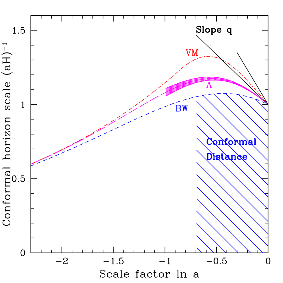
Figure 1: Visualization of dark energy cosmologies becomes intuitive in this diagram of the conformal Hubble scale vs. the logarithmic scale factor. Curves are shown for three different models, all flat with matter density $\Omega_{m}=0.3$: a cosmological constant $\Lambda$, a braneworld cosmology (BW), and vacuum metamorphosis (VM). The area under a curve between any two scale factors is the conformal distance, $\eta=d_{\rm lum}/(1+z)$, here shown by the diagonally shaded area for the braneworld model from today to $z=1$. The slope of a curve indicates acceleration or deceleration, with the slope today being $q_{0}$. This is shown for the $\Lambda$ curve by the long tangent, with $q_{0}=-0.55$. The shorter line shows $q_{0}=-1$; slopes greater than this represent a superaccelerating expansion. Note that while VM is a phantom ($w<-1$) model, it does not yet superaccelerate since the total equation of state is currently more positive than $-1$. The dense shading around the $\Lambda$ curve represents 95% confidence level constraints possible with SNAP, clearly mapping both accelerating and decelerating phases and distinguishing dark energy physics.

4 Ghosts in the Dark

With the next generation data, such as the densely shaded region around the $\Lambda$ curve of Fig. 1 representing the 95% confidence limit of SNAP, we can hope to reveal the nature of dark energy. As one example, we consider in this section the properties of a scalar field. A canonical scalar field $\phi$ with Lagrangian ${\cal L}=(1/2)\partial_{\mu}\phi\partial^{\mu}\phi-V(\phi)$ has an energy density $\rho=(1/2)\dot{\phi}^{2}+V$ and pressure $p=(1/2)\dot{\phi}^{2}-V$, where $V$ is the scalar field potential.

General relativity instructs us that the gravitating mass is proportional to $\rho+3p$, so we can obtain an answer to our introductory question if the ratio $w\equiv p/\rho<-1/3$. That is, for an equation of state ratio (EOS) $w<-1/3$, the field acts to accelerate the expansion. The quantity $w(z)$ plays a central role in understanding dark energy. In particular, both its value at any one time and its dynamics are important. The standard approximation for taking both of these into account is the form

$$w(z)=w_{0}+w_{a}(1-a),$$ (3)

where the scale factor is related to the redshift through $a=(1+z)^{-1}$. This form has been shown to capture the essence of quintessence for a wide variety of models [3].

Given the equation of state, one can formally obtain the energy density, the potential, the field dynamics, etc. However in practice, this is nearly impossible, not merely because of observational uncertainties, but due to the intrinsic nature of our accelerating universe. The field dynamics is given by

$$\dot{\phi}\sim\sqrt{(1+w)\rho}\sim HM_{P}\sqrt{1+w},$$ (4)

where $H=\dot{a}/a$ is the Hubble parameter and $M_{P}$ is the Planck energy. Since observations indicate that $1+w\ll 1$, then the field has only rolled $\Delta\phi\sim\dot{\phi}/H\ll M_{P}$ during the epoch when dark energy significantly affects the universe. Thus reconstruction of the potential is prevented.

In a recent breakthrough, Caldwell & Linder [4] realized that one can still use the field dynamics to categorize the nature of the physics responsible for the acceleration. Measurements of the dynamics to a precision $\sigma(w^{\prime}=\dot{w}/H)\approx 2(1+w)$ can distinguish between two distinct classes of “freezing” fields and “thawing” fields, with different physical origins. The time variation $w^{\prime}=-w_{a}/2$ in the parameterization of Eq. (3). Note that without measurement of dynamics, only knowing an averaged value $\langle w\rangle$, say, the physics is almost completely obscured. In particular, the entire “thawing” half of phase space would be mistaken for a cosmological constant.

While the categorization strictly holds for canonical scalar fields, research in progress shows it to be more general. But what about the possibility of $w<-1$, called phantom fields? These are often shunned due to “bad physics”, such as ghosts or imaginary mass particles and instabilities. The consequences of $w<-1$ for our universe [5] are remarkably similar to the definition of “bad” given in the 1984 movie Ghostbusters: “imagine all life as you know it stopping instantaneously and every molecule in your body exploding at the speed of light”!

However we must allow the data to lead us where it would. Moreover, various ways of obtaining at least an effective $w<-1$ without “bad” physics have been theorized. This ghostbusting includes

• Vacuum metamorphosis [6]

• Coupled dark energy [7, 8, 9, 10]

• Curvature plus $\Lambda$ [11]

• Braneworld plus $\Lambda$ [12, 13]

• Climbing field [14]

Finally, any modification of the Friedmann expansion equation can be written in terms of an effective EOS [15]. Defining the deviation from the usual Friedmann equation, $\delta H^{2}\equiv(H/H_{0})^{2}-\Omega_{m}a^{-3}$, simple examples include modifications depending solely on matter density, i.e. without any additional physical component in the universe:

$$\delta H^{2} = A(\rho_{m})^{n}\quad\Rightarrow\quad w=-1+n$$ (5)

$$\delta H^{2} = (8\pi/3)f(\rho_{m})\quad\Rightarrow\quad w=-1+d\ln f/d\ln\rho_{m}$$ (6)

From any such effective $w(z)$ one can in turn construct an effective potential.

5 The New Cosmology

While the EOS describes the expansion history of the universe and contains critical clues to the fundamental physics, one still needs an underlying theory to specify the presence of microphysics such as field perturbations, or to distinguish between physical origins. That $w(z)$ is such a general language is a feature, but also a bug, preventing us from distinguishing two models with identical expansion histories (see [10] for a detailed discussion). Fortunately, the growth history of matter density perturbations gives another window on dark energy.

Within general relativity, the perturbation growth is a function of the expansion history (plus perturbations in components other than matter, but these are expected to be negligible). But more generally the growth also depends on the gravitation theory. So we can distinguish the effects of dark energy as a physical component vs. those from a modification of gravity. For a model independent approach, Linder [10] proposed following the physics by incorporating the expansion effects via $w(z)$ and separately parameterizing the effects of gravity.

The linear growth factor $g(a)=(\delta\rho_{m}/\rho_{m})/a$ was found to be superbly approximated by

$$g(a)=e^{\int_{0}^{a}d\ln a\,[\Omega_{m}(a)^{\gamma}-1]}.$$ (7)

This is valid over a wide range of cosmologies to 0.05-0.2%. The new parameter, the growth index $\gamma$, measures the modification of gravity: for scalar fields within general relativity, $\gamma=0.55+0.05[1+w(z=1)]$; for a braneworld model though $\gamma=0.68$.

Beyond linearity, the growth of nonlinear matter structures such as galaxies and clusters of galaxies must be understood in dark energy cosmologies if they are to be used to probe dark energy. This requires a large suite of cosmological simulations covering a wide range of parameter space, especially since current fitting formulas for the mass power spectrum, say, are accurate to only $\sim 10\%$, and that primarily for cosmological constant universes. However, [16] discovered a method for improving the accuracy by almost an order of magnitude, at the same time speeding up the parameter space coverage by $\sim 100$. By matching the linear growth factor at two epochs, and $\Omega_{m}h^{2}$, they obtain accuracy better than 1.5% in the nonlinear power spectrum. Their method automatically matches CMB constraints also. This offers the hope of rapid development in the accurate calculation of quantities depending on the power spectrum (such as weak gravitational lensing measurements of large scale structure mass growth) over a variety of dark energy models.

Thus, cosmological measurements giving the expansion history (e.g. through supernovae) and the growth history (e.g. through weak gravitational lensing), working together, promise real hope to reveal the origin of dark energy. A next generation dark energy experiment must include both approaches to understand the nature of the new physics.

We illustrate this in Fig. 2. If we “weigh” dark energy in a diagram of dimensionless vacuum energy density vs. matter density, we need to remember that this assumes a cosmological constant is the dark energy; if we merely allow for a “springiness” of space $w\neq-1$, then the parameter estimation contours will increase. However we have no evidence for or expectation that $w$ is constant: time variation is generic, the “stretchiness” of the spring. Merely allowing for this possibility blows up the confidence region and we must employ additional data sets to constrain it. This is the power of complementarity – it allows us to be more physically reasonable, not to impose a priori constraints but let the data guide the way.

We can pinpoint the physics through measuring the dynamics $w_{a}$. Suppose then we allow for the presence of spatial curvature; again the constraints weaken and again we need to bring in complementary data. Suppose then we allow for modification of gravity, e.g. in the model independent parameter space of $w_{0}$, $w_{a}$, $\gamma$….

We refer to this process of relaxing the assumptions imposed on the physics and then combining additional probes as the ladder of constraints. To achieve true understanding of the nature of our universe, we require next generation experiments utilizing all the robust cosmological techniques we have. It will be an exciting decade as we learn to see darkness.

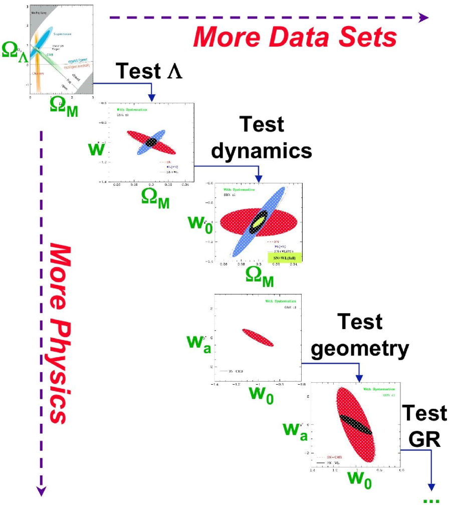
Figure 2: Assumptions imposed on dark energy physics allow strong constraints from data, but are often unjustified given our ignorance of dark energy. Relaxing these priors sometimes dramatically increase the uncertainties – as when avoiding assumption that the equation of state is constant – but allows us to test for important physics. The addition of robust, complementary, systematics controlled data sets, again constrains the nature of dark energy. (This diagram is intended to be illustrative only, not quantitative, but does include systematics.) This “ladder” of advancing the physics and the data hand in hand represents the new cosmology of seeing darkness.

I thank the organizers of TAUP2005 for the invitation and hospitality. I gratefully acknowledge Gary Bernstein, Dragan Huterer, and Masahiro Takada for information enabling Fig. 2. This work was supported in part by the Director, Office of Science, US Department of Energy under grant DE-AC02-05CH11231.

References

References

- [1] Linder E V 2005 in DARK2004, 5th International Heidelberg Conference, ed. Klapdor-Kleingrothaus H V (Springer Verlag) [arXiv: astro-ph/0501057]
- [2] SNAP http://snap.lbl.gov ; Aldering G et al arXiv: astro-ph/0405232
- [3] Linder E V 2003 Phys. Rev. Lett. 90 091301 [arXiv: astro-ph/0208512]
- [4] Caldwell R R and Linder E V 2005 Phys. Rev. Lett. 95 141301 [arXiv: astro-ph/0505494]
- [5] Caldwell R R, Kamionkowski M, and Weinberg N N 2003 Phys. Rev. Lett. 91 071301 [arXiv: astro-ph/0302506]
- [6] Parker L and Raval A 2000 Phys. Rev. D 62 083503 [arXiv: gr-qc/0003103]
- [7] Turner M S 1985 Phys. Rev. D 31 1212
- [8] Linder E V 1988 Astr. Astroph. 206 175
- [9] Amendola L and Quercellini C 2004 Phys. Rev. Lett. 92 181102 [arXiv: astro-ph/0403019]
- [10] Linder E V 2005 Phys. Rev. D 72 043529 [arXiv: astro-ph/0507263]
- [11] Linder E V 2005 Astropart. Phys. 24 391 [arXiv: astro-ph/0508333]
- [12] Lue A and Starkman G D 2004 Phys. Rev. D 70 101501 [arXiv: astro-ph/0408246]
- [13] Csaki C, Kaloper N, Terning J 2005 Annals Phys. 317 410 [arXiv:astro-ph/0409596]
- [14] Csaki C, Kaloper N, Terning J 2005, arXiv:astro-ph/0507148
- [15] Linder E V 2004 Phys. Rev. D 70 023511 [arXiv: astro-ph/0402503]
- [16] Linder E V and White M 2005 Phys. Rev. D 72 061304(R) [arXiv: astro-ph/0508401]