The Volume Fraction of Ionized Intergalactic Gas at Redshift z=6.5

Abstract

The observed number density of Lyman-$\alpha$ sources implies a minimum volume of the inter-galactic medium that must be ionized, in order to allow the Lyman-$\alpha$ photons to escape attenuation. We estimate this volume by assigning to each Lyman-$\alpha$ emitter the minimum Stromgren sphere that would allow half its Lyman-$\alpha$ photons to escape. This implies a lower limit to ionized gas volume fraction of 20-50% at redshift z=6.5. This is a lower limit in two ways: First, we conservatively assume that the Lyman-$\alpha$ sources seen (at a relatively bright flux limit) are the only ones present; and second, we assume the smallest Stromgren sphere volume that will allow the photons to escape. This limit is completely independent of what ionizing photon sources produced the bubbles. Deeper Lyman-$\alpha$ surveys are possible with present technology, and can strengthen these limits by detecting a higher density of Lyman-$\alpha$ galaxies.

1 Introduction

The epoch of reionization marks a phase transition in the universe, when the intergalactic medium was ionized. Recent observations of $z>6$ quasars show a Gunn-Peterson trough (Gunn & Peterson 1965) implying that the reionization of intergalactic hydrogen was not complete until $z\approx 6$ (Becker et al 2001, Fan et al 2002). Yet microwave background observations imply substantial ionization as early as $z\gtrsim 15$ (Spergel et al 2003; Kogut et al 2003). Transmitted flux seen in some quasar spectra also implies inhomogenities in the ionized gas (Oh & Furlanetto 2005; White et al. 2005). These results can be reconciled if reionization occurred twice (e.g., Cen 2003), slowly (e.g. Gnedin 2004) or was substantially inhomogenous (Malhotra et al. 2005, Oh & Furlanetto 2005, Cen 2005). Information on the state of the inter-galactic gas— the ionized fraction, and spatial distribution of ionized gas— is needed, but is scant.

Lyman-$\alpha$ emitters as tests of ionized IGM

Lyman-$\alpha$ emitting galaxies provide another tool for probing reionization, which is independent of and complementary to of the CMBR and Gunn-Peterson diagnostics. Lyman-$\alpha$ visibility tests offer a local probe of neutral fractions $x_{HI}\sim 30\%$ (Malhotra & Rhoads 2004 (MR04)), while the Gunn-Peterson trough saturates at $x_{HI}\sim 1\%$,(Fan et al 2002), and the CMBR polarization provides an integral constraint of the ionized gas along the line of sight.

Because Lyman-$\alpha$ photons are resonantly scattered by neutral hydrogen, Lyman-$\alpha$ line fluxes are attenuated for sources in a significantly neutral ($\langle x_{HI}\rangle\sim 0.1$) intergalactic medium (IGM) (Miralda-Escudé 1998, Loeb & Rybicki 1999, Haiman & Spaans 1999). To zeroth order this should produce a decrease in Lyman-$\alpha$ galaxy counts at redshifts beyond the end of hydrogen reionization (Rhoads & Malhotra 2001 (RM01)). This does not mean that Lyman-$\alpha$ emitters will suddenly become invisible at some redshift, but rather that Lyman-$\alpha$ flux is strongly attenuated. We consider three physical effects that modify the attenuation of the Lyman-$\alpha$ flux.

Effect of ionized bubbles

Each galaxy creates a local bubble of ionized gas. If this is large enough, Lyman-$\alpha$ photons are redshifted by the time they reach the neutral boundary and thus can escape. Consider a galaxy in a Stromgren sphere of radius $R_{ss}$, surrounded by a fully neutral IGM. The line center optical depth due to scattering by the damping wing of neutral gas outside the galaxy’s Stromgren sphere is given by $\tau=1.2\hbox{pMpc}/R_{ss}$ (e.g., RM01 ). Thus, transmission becomes significant when the physical radius of the HII region is $\gtrsim 1.2\hbox{pMpc}$ (correpsonding to $\gtrsim 9\hbox{cMpc}$ at redshift $z=6.5$),

For wavelengths separated from line center by $\Delta\lambda_{em}$, the optical depth due to neutral IGM damping wing is

$$\tau=1.2\hbox{pMpc}\times\left(R_{ss}+{\Delta\lambda_{em}\over\lambda_{0}}{c\over H}\right)^{-1}$$ (1)

where $c$ is lightspeed and where the Hubble constant $H\approx 760{\rm\,km\,s^{-1}\,Mpc^{-1}}\times[(1+z)/7.5]^{3/2}$ for a flat cosmology with $H_{0}=71{\rm\,km\,s^{-1}\,Mpc^{-1}}$, $\Omega_{m}=0.27$, and $\Omega_{\Lambda}=0.73$ (see Spergel et al 2003).

The size of a typical Stromgren sphere that an isolated galaxy creates in the IGM can be directly related to its Lyman-$\alpha$ luminosity $L_{Ly\alpha}=10^{43}L_{43}{\rm\,erg\,s^{-1}}$, its age $t=10^{8}t_{8}\hbox{yr}$, and the fraction $f_{\rm esc}$ of its ionizing photons that escape the galaxy to ionize the surrounding IGM (thereby becoming unavailable for Lyman-$\alpha$ line production) (RM01). The result, conservatively ignoring recombination, is

$$R_{ss}\approx{0.7\hbox{pMpc}\over 1+z}\left\{L_{43}t_{8}\left(f_{\rm esc}\over 1-f_{\rm esc}\right)\right\}^{1/3}~{}~{}~{}.$$ (2)

Stellar population models for narrowband-selected Lyman-$\alpha$ emitting galaxies require $t_{8}\lesssim 1$ (and usually $t_{8}\ll 1$) to produce the observed range of Lyman-$\alpha$ line equivalent widths (Malhotra & Rhoads 2002, MR02). The luminosity function for Lyman-$\alpha$ galaxies at $z\approx 6$ shows $L_{*}\sim 10^{42.6}{\rm\,erg\,s^{-1}}$ (MR04), so that galaxies with $L_{43}\gg 1$ are rare. Inserting $t_{8}\lesssim 1$ and $L_{43}\lesssim 1$ into equation 2 and comparing the result to equation 1, we see that $\tau\gtrsim 2$ at line center even for reasonably bright Lyman-$\alpha$ galaxies, and that these galaxies’ Stromgren spheres are not sufficient to prevent Lyman-$\alpha$ line suppression by an order of magnitude or more if the surrounding IGM is neutral.

Velocity Offsets

The observed Lyman-$\alpha$ line is usually asymmetric (e.g. Rhoads et al 2003, Dawson et al 2004) and offset to the red compared to other lines (e.g., Shapley et al. 2003). This offset is likely caused by absorption or scattering of Lyman-$\alpha$ photons in the blue wing of the emission line in the interstellar medium of the emitting galaxy, combined with gas motions (or outflows) in that medium. Resonant scattering by the surrounding IGM will further suppress the blue wing of the line, and accentuate the asymmetry. The typical observed velocity offsets for LBGs with Lyman-$\alpha$ emission is $\sim 360\hbox{km s${}^{-1}$}$, although the velocity offsets decrease for galaxies with higher equivalent widths in the Lyman-$\alpha$ emission (Shapley et al. 2003). Such an offset can be incorporated in equation 1 using $\Delta\lambda_{em}=\lambda_{0}v_{w}/c$, where $v_{w}$ (the “wind” velocity) denotes the offset of the Lyman-$\alpha$ line relative to the systemic velocity of the emitting galaxy.

If we describe the intrinsic profile as $f_{\lambda}(\lambda_{0}+\delta\lambda)$, where $\lambda_{0}=1215.67$Å is the rest Lyman-$\alpha$ wavelength, then the unabsorbed line flux is $F_{0}=\int_{-\infty}^{\infty}f_{\lambda}(\lambda_{0}+\delta\lambda)d(\delta\lambda)$. The absorbed line flux is $F=\int_{-\infty}^{\infty}\exp[-\tau(\delta\lambda)]f_{\lambda}(\lambda_{0}+\delta\lambda)d(\delta\lambda)$, and the transmission factor is $T\equiv F/F_{0}$, which is calculated by integrating over the line profile.

Santos (2004) has calculated the transmission factor for a large range of model Lyman-$\alpha$ line properties and IGM models His results show that $T\lesssim 1/3$ for a wide range of plausible models, even including those with $v_{w}=360\hbox{km s${}^{-1}$}$. Models with $v_{w}=0$ invariably show $T\ll 1/3$, unless the IGM is largly ionized. Moreover, the variation of $T$ with $v_{w}$ is fairly slow for $v_{w}>360\hbox{km s${}^{-1}$}$; that is, a large increase of $\langle v_{w}\rangle$ would be required to substantially raise $\langle T\rangle$.

Galaxy clustering

Even though a single Lyman-$\alpha$ galaxy does not produce a large enough Stromgren sphere, there is a possibility that fainter galaxies clustered around the observed Lyman-$\alpha$ galaxy would contribute enough photons to make the HII regions around the cluster reach the critical size. This would require roughly 10-60 times more photons than produced by a typical Lyman-$\alpha$ galaxies observed (Wyithe & Loeb 2005, Haiman & Cen 2005, Furlenatto et al. 2004) So far the evidence for such clustering is mixed: Malhotra et al. 2005 see clustering in the Hubble Ultra Deep field which was chosen to include a 25th magnitude galaxy at z=5.8, so do Stiavelli et al 2005 around a SDSS quasar at z=6.2; but Rhoads et al. (in prep) see no significant excess around an actual z=6.5 Lyman-$\alpha$ galaxy.

We here introduce a new version of the Lyman-$\alpha$ reionization test wherein aach observed Lyman-$\alpha$ galaxy is seen because the IGM near that galaxy is ionized in an otherwise neutral medium. Each Lyman-$\alpha$ galaxy thus implies the presence of a certain volume of ionized IGM. We combine this ionized volume per source with the observed number density of Lyman-$\alpha$ galaxies to obtain a lower bound on the volume ionized fraction of the IGM. This limit is completely independent of whether the ionizing photons come from the Lyman-$\alpha$ galaxy, its unseen neighbors, or any other source.

2 Ionized volume estimates

Calculating the Transmission

We need to calculate the Lyman-$\alpha$ flux transmission expected from a galaxy with a given Stromgren sphere radius, Lyman-$\alpha$ line velocity offset, and IGM neutral fraction. To do so, we must make some reasonable assumptions about the line width and shape. Observed Lyman-$\alpha$ emission lines from high redshift galaxies are well described by a truncated Gaussian profile (Hu et al 2004, Rhoads et al 2004):

$$f_{\lambda}(\lambda_{0}+\delta\lambda)=\left\{\begin{array}[]{ll}{2F_{0}\over\sqrt{2\pi}\sigma}\exp\left(-{(\delta\lambda)^{2}\over 2\sigma^{2}}\right)&\hbox{if }\delta\lambda\geq 0\\ 0&\hbox{if }\delta\lambda<0\end{array}\right.$$ (3)

where $\lambda_{0}=1215.67(1+v_{w}/c)$Å is the Lyman-$\alpha$ central wavelength in the frame of the IGM surrounding the galaxy, and the unabsorbed line flux is $F_{0}$. The absorbed line flux is $F=\int_{-\infty}^{\infty}\exp[-\tau(\delta\lambda)]f_{\lambda}(\lambda_{0}+\delta\lambda)d(\delta\lambda)$, and the transmission factor is $T\equiv F/F_{0}$. We set $\sigma=1.49$Å, or rest frame FWHM of $1.75$Å (from the truncation point $\lambda_{0}$ to the half-peak point on the red side of the line) - chosen to match typical observed high redshift Lyman-$\alpha$ lines.

We determined $T$ by numerical integration for a grid of $v_{w}$ and $R_{ss}$. We then inverted the result to determine the Stromgren sphere radii corresponding to 25%, 33%, 50%, and 70% transmission for a range of Lyman-$\alpha$ velocity offsets $v_{w}$. The result is summarized in figure 1.

Figure 1: This figure shows the minimum radius of the ionized bubble needed for 70% (dot dashed line), 50% (solid line), 33% (short dashed line) or 25% (long dashed line) of Lyman-$\alpha$ line flux to escape as a function of the velocity offset between the Lyman-$\alpha$ emission line and the intrinsic velocity of the galaxy. Currently, a transmission factor of less than 50% is ruled out by MR04, and the best guess for velocity offset is $\approx 350\hbox{km s${}^{-1}$}$; which would imply $R_{ss}=0.93$ physical or 7 comoving Mpc.

The Minimum Ionized Fraction: Analytic results

We next combine our calculated minimum Stromgren sphere radii with the observed number density of $z\approx 6.5$ Lyman-$\alpha$ emitting galaxies to place a lower bound on the volume ionized fraction of the intergalactic medium. The problem is closely related to the void probability function, or to a counts-in-cells formalism. The volume neutral fraction $x_{V,\hbox{\scriptsize n}}\equiv 1-x_{V,\hbox{\scriptsize ion}}$ can be found by calculating the probability that an arbitrary point in space lies in a void of radius $\geq R_{ss}$ in the Lyman-$\alpha$ galaxy distribution, or (equivalently) by calculating the probability that a randomly placed, spherical cell of radius $R_{ss}$ will contain no Lyman-$\alpha$ galaxies.

The zero order estimate of the ionized volume fraction is simply $x_{V,\hbox{\scriptsize ion}}\approx{\cal F}\equiv nV_{ss}$. Here $n$ is the volume number density of the detected Lyman-$\alpha$ emitting galaxies, $V_{ss}=(4\pi/3)R_{ss}^{3}$ is the volume of the minimum size Stromgren sphere that renders them visible, and ${\cal F}$ is the filling factor of these spheres. The estimate $x_{V,\hbox{\scriptsize ion}}\approx{\cal F}$ is accurate for $x_{V,\hbox{\scriptsize ion}}\ll 1$. At larger ionized fractions, we need to correct for overlap of the Stromgren spheres.

If the locations of the Lyman-$\alpha$ galaxies are uncorrelated, the residual neutral volume fraction becomes $x_{V,\hbox{\scriptsize n}}=\exp(-{\cal F})$ and the corresponding ionized fraction is $x_{V,\hbox{\scriptsize ion}}=1-\exp(-{\cal F})=\sum_{j=1}^{\infty}(-1)^{j-1}{\cal F}^{j}/j!$.

The degree of overlap will be further enhanced by spatial correlations among galaxies. To account for this overlap, we can assume that the observed Lyman-$\alpha$ emitters are drawn from a distribution with two-point angular correlation function $\xi(r)\approx(r/r_{0})^{-\gamma}$. We take values $r_{0}\approx 4\hbox{cMpc}$ and $\gamma=1.8$, which are typical of high redshift galaxy populations and in particular are consistent with observed Lyman-$\alpha$ galaxy populations (e.g., Ouchi et al. 2003, Kovac et al. in prep.). This correlation function implies that the mean number of neighbors within distance $r$ of an arbitrarily selected galaxy should be $\langle N_{p}\rangle=(4\pi/3)r^{3}n\left(1+3(r/r_{0})^{-\gamma}/(3-\gamma)\right)$ (Peebles 1980, eq. 31.8). Given a pair of ionized spheres with radius $R_{ss}$, whose centers are separated by distance $r$ (with $0\leq r/R_{ss}\leq 2$), the volume of their overlap region is $V_{ss}\times\left(1-0.75(r/R_{ss})+(r/R_{ss})^{3}/16\right)$. We integrate the expected volume “lost” to overlap within a survey by combining the two foregoing results:

$$\begin{array}[]{lll}x_{V,\hbox{\scriptsize ion}}&=&{\cal F}-{1\over 2}{\cal F}^{2}\left\{1+3\left(R_{ss}\over r_{0}\right)^{-\gamma}\left[{2^{3-\gamma}\over 3-\gamma}-{3\over 4}{2^{4-\gamma}\over 4-\gamma}{2^{6-\gamma}\over 16(6-\gamma)}\right]\right\}\end{array}$$ (4)

While this calculation accounts for correlations, it omits third order and higher terms in ${\cal F}$. The coefficient for the ${\cal F}^{3}$ term would depend on the three point correlation function. Thus equation 4 will tend to underestimate the volume ionized fraction, and is conservative.

Minimum Ionized Fraction: Numerical simulations

To achieve accurate results at higher source densities, we simulated correlated distributions of galaxies and directly calculated the volume fraction enclosed by the union of their Stromgren spheres. We performed these calculations for a range of correlation lengths, Stromgren sphere sizes, and source densitites. We generated the set of correlated $(x,y,z)$ triples using a Mandelbrot-Levy random walk prescription (see Peebles 1980, section 62). A power law distribution of step lengths $s$, $p(s)\propto s^{-1.2}$, ensures a power law correlation function with the desired slope $\gamma=-1.8$. The correlation length $r_{0}$ is related to the minimum step length (which is always $\ll R_{ss}$ and $\ll r_{0}$) and to the number of independent random chains occupying the sample volume. To tune the correlation length to a desired value, we vary the number of chains used and also (for small correlation lengths) add a suitable number of entirely uncorrelated $(x,y,z)$ triples.

We verified that this prescription generated the desired two-point correlation properties. The volume used for the simulations was $\sim 10^{6}\hbox{cMpc}^{3}$, and the volume fraction was calculated on a grid with cell size $=R_{ss}/2$. (A smaller cell size does not significantly change the results) Finally, we verified that the simulations reproduce the analytic results for an uncorrelated distribution at any filling factor, and for a correlated distribution at ${\cal F}\lesssim 1$ (where the ${\cal F}^{3}$ and higher terms are small).

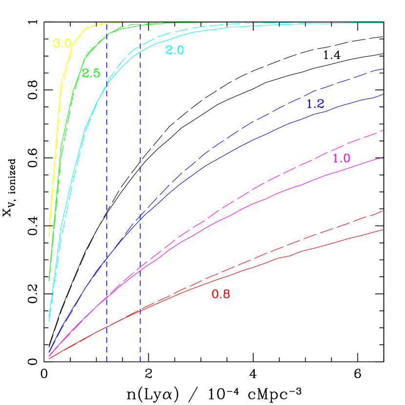
Figure 2: The volume ionized fraction as a function of observed Lyman-$\alpha$ source density is plotted for a range of minimum Stromgren sphere sizes and correlation lengths. From highest to lowest, these sets of curves correspond to $R_{ss}=3.0\hbox{pMpc}$ (yellow), $2.5\hbox{pMpc}$ (red), $2.0\hbox{pMpc}$ (magenta), $1.4\hbox{pMpc}$ (green), $1.2\hbox{pMpc}$ (cyan), $1.0\hbox{pMpc}$ (black) and $0.8\hbox{pMpc}$ (blue). For each set of curves, the line style indicates the correlation length: $r_{0}=0$ (dotted), and $4\hbox{cMpc}$ (solid). Vertical lines at $1.2\times 10^{-4}$ and $1.8\times 10^{-4}\hbox{cMpc}^{-3}$ mark the range of Lyman-$\alpha$ number density observed by Taniguchi et al (2004). For the best-guess parameters $1\lesssim R_{ss}\leq 1.4\hbox{pMpc}$ and $r_{0}\approx 4\hbox{cMpc}$, the Taniguchi data imply a lower bound of $0.2$ to $0.5$ on $x_{V,\hbox{\scriptsize ion}}$.

Results of the simulations are shown in figure 2, where we show curves of $x_{V,\hbox{\scriptsize ion}}$ as a function of the Lyman-$\alpha$ galaxy number density for a plausible range of $R_{ss}$ and $r_{0}$ values. Were we to plot $x_{V,\hbox{\scriptsize ion}}$ as a function of ${\cal F}$ (rather than $n$), we would see that $x_{V,\hbox{\scriptsize ion}}$ is a function of just two variables, ${\cal F}$ and the ratio $(r_{0}/R_{ss})$, as one would expect from the discussion in section 2.

Effect of a Partly Ionized Ambient Medium

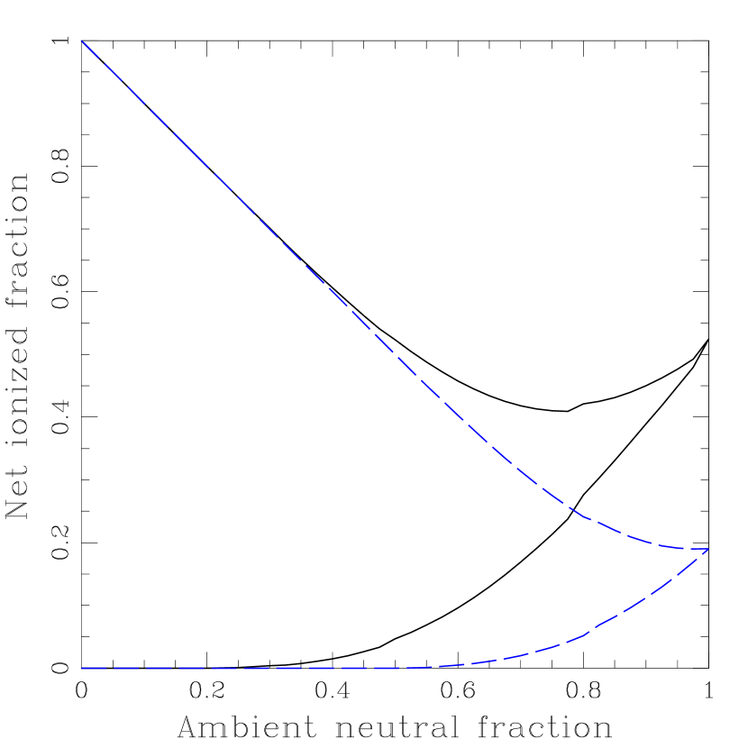
Figure 3: The ionized gas fraction in the IGM is plotted as a function of the neutral fraction in the ambient medium (outside Stromgren spheres). We have assumed a number density of $1.5\times 10^{-4}\hbox{cMpc}^{-3}$ (Taniguchi et al 2004). Two solid (black) curves show the result for $v_{w}=0$. The lower curve shows the amount of ionized gas enclosed in Stromgren spheres around Lyman-$\alpha$ galaxies, and the upper curve shows the total ionized gas fraction (including that in the ambient medium). The dashed (blue) curves show the same quantities for $v_{w}=360\hbox{km s${}^{-1}$}$.

Up to now, we have considered Stromgren spheres embedded in a fully neutral ambient intergalactic medium. If this medium is already partially ionized outside the bubbles, then Lyman-$\alpha$ flux is transmitted more easily, and the Stromgren spheres required to achieve a particular Lyman-$\alpha$ transmission are smaller. However, this scenario requires a large amount of ionized gas mixed into the ambient medium. Figure 3 shows the net ionized fraction of ionized gas (counting the Stromgren spheres + ambient ionized gas) as a function of ambient neutral fraction for $v_{w}=0$ and $360\hbox{km s${}^{-1}$}$

3 Summary and Future outlook

Observations of Lyman-$\alpha$ emitters provide a powerful method to probe the neutral fraction of the IGM and the volume of the ionized gas. In an earlier paper we explored the effect on the Lyman-$\alpha$ luminosity function and constrained the average neutral fraction of the IGM to be $\langle{x_{\hbox{\scriptsize n}}}\rangle<30$–$50\%$ (MR04, see also Stern et al. 2005). Further investigations by Haiman & Oh 2005 and Furlennato et al. 2005 agreed with these estimates. In this letter we place a lower limit on the volume in ionized IGM $x_{V,\hbox{\scriptsize ion}}=20-50\%$ for best known parameters of transmission factor $T=0.5$, source density $n(ly\alpha)=10^{-4}$, and $v_{w}=360-0\hbox{km s${}^{-1}$}$.

With better observations, these limits can be substantially improved. Currently, the largest Lyman-$\alpha$ galaxy sample at z=6.5 comes from Subaru observations (Taniguchi et al. 2005) which reach just about $\L_{*}$. Going deeper is then expected to yield a higher density of Lyman-$\alpha$ emitters. If the current observed number density of sources could be increased by a factor of 2 or 3 with deeper observations, the lower limit to $x_{V,\hbox{\scriptsize ion}}$ would increase by a factor of 2. Bigger samples (both at z=6.5 and z=5.7) would also improve the estimate of the attenuation factor. MR04 concluded that attenuation of a factor of two was marginally allowed by present data. If we could reduce this limit to 1.4, i.e a transmission factor of 70%, we would conclude that the minimum Stromgren sphere radius needed would be 3 pMpc for offset velocity of zero, and 2.6 pMpc for a velocity offset of 350 km s^-1 (Figure 1). In that case the Taniguchi et al. 2005 data would imply nearly $x_{V,\hbox{\scriptsize ion}}=100\%$. Moreover, we should not forget that we are using the smallest value of $R_{SS}$ that allows the transmission of the Lyman-$\alpha$ line. The ionized bubbles could certainly be larger.

Measurement of the velocity offset between Lyman-$\alpha$ redshift and systematic velocity of the galaxy will allow us to further refine the Stromgren sphere radius (see Figure 1). Currently our estimates come from such measurements on Lyman break galaxies (LBGs), for which the higher the EW of the Lyman-$\alpha$ line, the smaller the velocity offset (Shapley et al. 2003). But the overlap between the LBG samples and the Lyman-$\alpha$ samples is minimal; only the LBGs with highest EW (EW $\approx 50$ Å) would even be selected by the Lyman-$\alpha$ searches using Narrow-bands. So it is plausible that the velocity offsets for the Lyman-$\alpha$ emitters (median EW $\approx 100$Å; (MR02, Dawson et al. 2004) would be even lower.

Spectroscopy of large, complete samples would also yield the information on their distribution and clustering in the line-of-sight dimension, which can be used to determine the overlap in the ionized bubble around the galaxies. Then we can go beyond the zeroth order estimate of $x_{V,\hbox{\scriptsize ion}}$ to learn about the topology of the ionized bubbles and thus determine whether substantial overlap has happened (Rhoads, in prep). Pre-overlap phases of reionization can also be detected by heightened correlation between Lyman-$\alpha$ sources (Furlanetto et al. 2005). If the sources required for ionizing photons are strongly clustered on $\approx 100cMpc$ scales as observed (Malhotra et al. 2005) or predicted (Cen 2005), we should see dramatic field-to-field variations in Lyman-$\alpha$ number density prior to reionization.

These tests only require the detection of statistically useful samples of Lyman-$\alpha$ emitters and are eminently practical with present technology at optical wavelengths, and their extension to redshifts $z>7$ through near-infrared observations is close at hand.

References

- (1) Becker, R. H., et al. (SDSS consortium), 2001, AJ 122, 2850
- (2) Cen, R. 2003, ApJ, 591, 12.
- (3) Cen, R. 2005, astro-ph/0507014.
- (4) Dawson, S., Spinrad, H., Stern, D., Dey, A., van Breugel, W., de Vries, W., & Reuland, M. 2002, ApJ 570, 92
- (5) Dawson, S., Rhoads, J., Malhotra, S. Stern, D., Dey, A., Spinrad, H., Jannuzi, B. T., Wang, J. X., & Landes, E. 2004, ApJ 617, 707
- (6) Fan, X., Narayanan, V. K., Strauss, M. A., White, R. L., Becker, R. H., Pentericci, L., & Rix, H.-W. 2002, AJ 123, 1247
- (7) Furlanetto, et al. 2004, ApJ, 613, 16.
- (8) Furlanetto, S., Zaldariaga, M., Hernquist, L., 2005, astro-ph/0507266
- (9) Gnedin, N. 2004, ApJ, 610, 9.
- (10) Gunn, J.E., Peterson, B.A., 1965, ApJ 142, 1633
- (11) Haiman, Z., Cen, R. 2005, ApJ 623, 627.
- (12) Haiman, Z., & Spaans, M. 1999, ApJ 518, 138
- (13) Hu, E. M., Cowie, L. L., , Capak, P., McMahon, r. g., Hayashino, T., & Komiyama, Y. 2004, AJ, 127,563.
- (14) Kogut, A., et al. 2003, ApJS, 148, 161.
- (15) Loeb, A. & Rybicki, G. B. 1999, ApJ 524, L527
- (16) Malhotra, S., & Rhoads, J. E. 2002, ApJ 565, L71 (MR02)
- (17) Malhotra, S., & Rhoads, J.E. 2004, ApJ 617, L5 (MR04).
- (18) Malhotra, S., Rhoads, J.E., Haiman, Z. et al. 2005, ApJ 626, p666.
- (19) Miralda-Escudé, J. 1998, ApJ 501, 15
- (20) Oh, P., Furlanetto, S, 2005, ApJ, 620, L9.
- (21) Ouchi, M, et al. 2003, 582, 60.
- (22) Peebles, P.J.E., 1980, Large Scale structure of the Universe, Princeton University Press.
- (23) Rhoads, J. E., Malhotra, S., Dey, A., Stern, D., Spinrad, H., & Jannuzi, B. T. 2000, ApJ 545, L85
- (24) Rhoads, J. E., & Malhotra, S. 2001, ApJ 563, L5 (RM01)
- (25) Rhoads, J. E., Dey, A., Malhotra, S., Stern, D., Spinrad, H., Jannuzi, B. T., Dawson, S., Brown, M. J. I., & Landes, E. 2003, AJ 125, 1006
- (26) Rhoads, J. E., Xu, C., Dawson, S., Dey, A., Malhotra, S., Wang, J. X. Jannuzi, B. T., Spinrad, H., & Stern, D. 2004, ApJ 611, 59
- (27) Santos, M. R. 2004, MNRAS, 349, 1137
- (28) Shapley, A., Steidel, C., Pettini, M., Adelberger, K, 2003, ApJ 588, 65.
- (29) Spergel, D. N., et al 2003, ApJS, 148, 175
- (30) Stern, D., Yost, S. A., Eckart, M. E., Harrison, F. A., Helfand, D. J., Djorgovski, S. G., Malhotra, S., & Rhoads, J. E. 2005, ApJ, 619, 12
- (31) Stiavelli, M. et al. 2005, ApJ, 626, L1.
- (32) Taniguchi, Y et al. 2005, PASJ 57, 165.
- (33) White, R., Becker, R.H., Fan, X., Strauss, M. 2005, AJ, 129, 2102.
- (34) Wyithe, J.S.B., Loeb, A., 2005, ApJ, 2005, 1.